Alison de Oliveira Moraes*
Institute of Aeronautics and Space São José dos Campos, Brazil [email protected]
Waldecir João Perrella
Technological Institute of Aeronautics São José dos Campos, Brazil [email protected]
*author for correspondence
Performance evaluation of
GPS receiver under equatorial
scintillation
Abstract: Equatorial scintillation is a phenomenon that occurs daily in the equatorial region after the sunset and affects radio signals that propagate through the ionosphere. Depending on the temporal and spatial situation, equatorial scintillation can represent a problem in the availability and precision of the Global Positioning System (GPS). This work is concerned with evaluating the impact of equatorial scintillation on the performance of GPS receivers. First, the morphology and statistical model of equatorial
scintillation is briely presented. A numerical model that generates synthetic
scintillation data to simulate the effects of equatorial scintillation is
presented. An overview of the main theoretical principles on GPS receivers
is presented. The analytical models that describe the effects of scintillation at receiver level are presented and compared with numerical simulations using a radio software receiver and synthetic data. The results achieved by simulation agreed quite well with those predicted by the analytical models. The only exception is for links with extreme levels of scintillation and when weak signals are received.
Keywords: Component tracking performance, GPS receiver, Ionospheric scintillation, Communication system simulation.
INTRODUCTION
Several environmental factors may affect GPS (Global Positioning System) performance, such as electromagnetic interference, multipath, atmospheric delay and ionospheric scintillation. Ionospheric Scintillation is responsible for a signiicant decrease in GPS accuracy, which may lead to a complete system failure (Beach, 1998). Ionospheric scintillations result in rapid variations in phase and amplitude of the radio signal, which crosses the ionosphere. Such a phenomenon is more usual near equatorial regions approximately from -20o to 20o of the globe and auroral zone from 55o to 90o of latitude. Apart from that, the scintillation activity has a temporal dependence, according to the local season and the solar cycle that has an 11-year period (Beach, 1998; Kintner et al., 2004). The ionospheric scintillation phenomenon in equatorial regions is known as equatorial scintillation. This kind of scintillation impacts predominantly by causing luctuations on the intensity of the signal (Beniguel et al., 2004). Equatorial scintillation usually takes place after sunset, affecting the GPS receiver performance, depending on its severity (Basu, 1981). The objective of this work is to evaluate the effects of equatorial scintillation on the code and carrier tracking loops of GPS receivers. Initially, an introduction to ionospheric behavior in equatorial zones is given;
followed by a statistical model presentation, which characterizes the amplitude scintillation. Following this, a receiver performance analysis is presented, as function of this effect. Based upon such an analysis, analytical models are used to represent the behavior and performance of GPS receivers. Finally, results of numerical simulations are presented and compared to analytical results.
FUNDAMENTALS OF IONOSPHERIC SCINTILLATION
Ionosphere
The ionosphere is the layer of the atmosphere where free electrons and ions are present in suficient quantities to affect the radio waves traveling through it. The structure of the ionosphere varies due to season, daily variation, solar production and the process of recombination among electrons. The ionosphere is sub-classiied in layers D, E, F1 and F2, according to the electrical density present. The D layer extends from 50km to 90km of altitude. It has a low electron density, vanishing during the night. The E layer extends from 90km to 140km in height and is basically produced by the solar X-rays, having a peak of electron density at 120km. The F1 layer extends from 140km to 200km and the main source of ionization is the solar extreme ultraviolet light (EUV). The F2 layer
Received: 06/08/09 Accepted: 29/09/09
Figure 1. Electrical density proile of ionosphere during day
and night.
Figure 2. Equatorial fountain that gives rise to the equatorial anomaly.
extends from 200km to 1000km and presents a region of maximum electron density at 350km (Kelley, 1989). These layers are a result of photochemical processes and plasma transportation. A typical electron density proile of the ionospheric layers during the daytime and the ionization during the evening hours is shown in Fig. 1.
At dusk, the electric ield, E, increases as the neutral winds, V, increases, and the ExB drift raises the F layer. This process is known as Pre-Reversal Enhancement when the base of the F layer is forced against the gravity, creating the Rayleigh-Taylor Instability, in which a heavier luid is held by a lighter one. When a perturbation happens, this equilibrium is broken and the lighter luid rises through the denser luid creating a bubble. In the region of the equatorial ionosphere these bubbles are called Equatorial Plasma Bubbles. The Equatorial Anomaly is responsible for the formation of the plasma density irregularities that result in the Equatorial Plasma Bubbles that lead to scintillation (Kintner et al., 2004).
STATISTICAL CHARACTERISTIC OF AMPLITUDE SCINTILLATION
The index that indicates the severity of amplitude scintillation is the S4. It is deined as the normalized variance of intensity of the received signal, given by
(1)
where I=AS2 is the intensity of the received signal. Based on studies of ionospheric scintillation data, it has been shown that amplitude scintillation might be modeled as a stochastic process that follows a Nakagami-m distribution, given by (Fremouw, Livingston and Miller, 1980)
(2)
where AS is the amplitude of the received signal, Γ() is the gamma function, and . The m parameter from Nakagami-m distribution and the S4 index are related by m=1/S42.
It is important to observe how the layers decay at night in the absence of photo-ionization. The F1 layer almost disappears while F2 and E layers still remain due to recombination and transportation.
Equatorial Scintillation
Equatorial scintillation happens when small-scale irregularities in the F region of the ionosphere affect the RF signals. Inluenced by the pressure gradients and gravity, the equatorial plasma present in the F2 layer is forced downward along the magnetic ield lines. This process creates a belt of enhanced electron density from 15o to 20o on both sides of the geomagnetic equator. This particular region where the electron density in enhanced is referred to as the Equatorial Anomaly. The process by which they are created is known as the Fountain Effect. This process is illustrated in Fig. 2, where the Equatorial Fountain is indicated by the ExB drift, which drives the plasma upward. This plasma is then diffused along
SYNTHETIC AMPLITUDE SCINTILLATION DATA
Based on Humphreys et al. (2008), a scintillation model has been implemented with the objective of simulating the scintillation effects on equatorial transionospheric radio signals such as the GPS ones. This model assumes that amplitude scintillation follows a Rice distribution. This assumption has been made because of the implementation simplicity of the Rice model. The Rice distribution is given by
p A
( )
S =2AS 1+K
(
)
Ω I0 2AS
K+K2
Ω ⎛
⎝
⎜ ⎞
⎠
⎟e−K−AS2(1+K) Ω (3)
where, AS ≥0,I0( ) is the modiied Bessel function of
zeroth order and K is Rician parameter. Although the Nakamami-m distribution, (2), is the one that best its the real scintillation data (Fremouw, Livingston and Miller, 1980). But in Humphreys et al. (2008), it is shown that Nakamami-m and Rice distribution are similar and they agree quite well with the empirical data for S4 <1, according to the chi-square tests. Thus, the Nakamagi-m distribution might be closely approximated by Rice distribution. This mapping is given by (Simon and Alouini, 2006),
K= m2−m m− m2−m (4)
Considering the expression
z t
( )
=zK + ξ( )
t (5)where
z
K is a complex constant and ξ( )t is a zero mean, gaussian process. From (5), the amplitude scintillation with a Rice distribution can be generated byAS
( )
t = z t( )
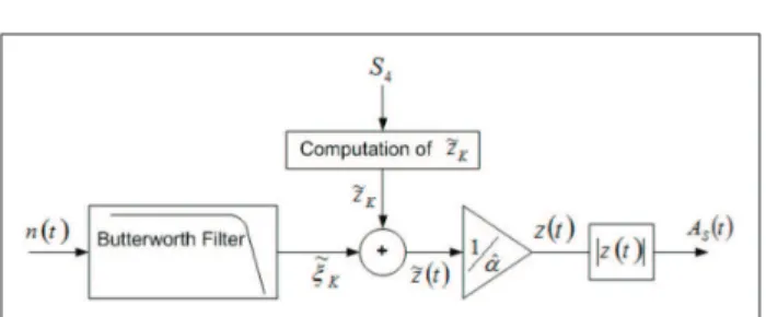
(6)The block diagram showing the mechanization process of scintillation simulator is illustrated in Fig. 3.
According to this process, a zero-mean white Gaussian noise n(t) is applied to a 2nd order Butterworth low pass ilter, with the response:
H(f)=1 1+ f Bd ⎛ ⎝⎜
⎞ ⎠⎟
4
(7)
where Bd= β 2πτ0 is the frequency bandwidth,
β=1.2396464 is a constant and τ0 is the decorrelation time of generated scintillation data. The iltered version of n t
( )
is denoted ξ(t), with varianceσξ
2
. The value of zK in (5) is responsible for controlling the level of scintillation in the simulator.
zK= 2σξ2K (8)
Based on (4) and the relation m=1/S42 it is possible to establish a relation between the scintillation index S4 and
the Rician parameter K, that is used to compute zK .
The constant zK is added to ξ(t), resulting in z t( )=ξ( )t+zK. The signal z t( ) is then normalized by α = E⎡⎣z t( )⎤⎦ , resulting in a synthetic scintillation data. An example of amplitude scintillation data generated by this model is shown in Fig. 4.
Figure 3. Mechanization process of scintillation simulator.
Figure 4. Example of scintillation for S4=0.68.
GPS RECEIVER
Figure 5. Architecture of GPS receiver (Ward, 1996).
and tracking of the received signal, providing the pseudo range and carrier phase information. The last section of the receiver is the Navigation Data Processing (NDP), this section has the task of calculating ephemeris data, GPS time, position and velocity (Ward, 1996).
Scintillations affect the performance of GPS receivers, in a notable way at the tracking loop level. Depending on the scintillation level, the receiver might increase the range measurement errors or can even lead to carrier loss of lock and code loops. In extreme cases, the scintillation can result in full disruption of the receiver.
The signal received from a generic GPS satellite, at the output of the FE that will be processed by the DSP section of the receiver is given as (Borre et al., 2007):
s (n)=A(n)C (n− τ)D(n− τ)cos(2πfFIt+ ϕ)+N(n) (9)
where A(n) is the amplitude of the received signal, C(n) is the satellite pseudorandom noise code (PRN), D(n) is the navigation data sequence,
τ
is the code delay, fFI is the intermediate frequency,ϕ
is the phase of the GPS carrier. In addition to the received signal, there is the termN
(
n
)
that represents the band-limited, stationary, Gaussian noise, with zero mean and power spectrum density.Carrier Tracking Loop
In order to demodulate the GPS navigation data successfully, it is necessary to generate an exact carrier wave replica. This task is usually executed in a GPS receiver by a phase locked loop (PLL). The model of PLL used on GPS receivers is based on a Costas suppressed carrier tracking loop, as illustrated in Fig. 6 (Ward, 1996).
In each arm of the Costas loop, the IF signal undergoes two multiplications. The irst one has the objective of wiping off
Figure 6. Block diagram of Costas carrier tracking loop.
the carrier of the received signal. The Costas tracking loop is insensitive to 180o phase shifts, which requires a second multiplication that wipes off the PRN code. The PRN code is generated by the code tracking loop. After the multiplications the signal in both arms is iltered by a pre-detection integrate and dump ilter. These signals are then used by the phase discriminator to determine the carrier phase error between the local generated replica and the received signal. The phase error computed by the discriminator is iltered and applied as a feedback to the NCO.
An important parameter in the evaluation of receiver performance is the tracking threshold point, which is the value where the loop stops working stably and loses the lock. When it happens, the phase error measurements become meaningless and the number of cycle slips increases. The exact point of this transition is hard to determine. Reasonable values to be assumed as a threshold, and mean time between cycle slips are given respectively by Holmes (1982):
σϕε2 lim = π
(
12)
2rad2
⎡⎣ ⎤⎦ (10)
T = π2ρεI02
( )
ρε 2Bn (11) where ρε=1 4σϕε2
is the signal-to-noise ratio of the loop.
Code Tracking LoopUnits
When there is no scintillation, the component of tracking error due to thermal noise in a PLL is given by,
σϕ2Th=C NBn 0
1+ 1
2Δt C N
(
0)
⎡⎣
⎢ ⎤
⎦
⎥ (14)
where Bn is the PLL single-sided noise equivalent bandwidth, C/N0 is the nominal carrier to noise density ratio and
Δ
t
is the pre-detection integration period.The equatorial scintillation presents indicative luctuation in the intensity of the received signal. This amplitude scintillation degrades the C/N0 and, as a consequence, increases the tracking error due to thermal noise. In (Conker et al., 2003), the effects of amplitude scintillation have been modeled, considering that this kind of scintillation follows a Nakagami-m distribution. Thus the thermal noise tracking error can be characterized by S4, according to the expression
σϕ2Th=
Bn 1+ 1
2Δt C N
(
0)
(
1−2S42)
⎛ ⎝
⎜ ⎞
⎠ ⎟
C N0
(
)
(
1−S42)
(15)
The term σϕ2Th in (13) is the one that most contributes to the PLL tracking error variance. Indeed, the other terms in (12), compared with σϕ2Th become negligible.
For the tracking error code delay at the output of DLL it is correct to afirm that στε
2 = σ
τ2Th , where στ2Th is the thermal noise component. In this case, there is no phase scintillation component, because according to Davies, 1990, a non-coherent DLL is not affected by the phase scintillation. In the absence of scintillation, the DLL tracking error code loop in function of the thermal noise is given by
στ2Th=2C NBnd 0
1+ 1 Δt C N0
⎡ ⎣
⎢ ⎤
⎦
⎥ (16)
In an analogous way to the PLL case, in (Conker et al., 2003), the effects of scintillation on the DLL is modeled using a Nakagami-m distribution to characterize tracking code error by function of amplitude scintillation index, S4, that is expressed as
στTh
2 =
Bnd 1+Δt C N1 0
(
)
(
1−2S42)
⎛ ⎝
⎜ ⎞
⎠ ⎟
2
(
C N0)
(
1−S42)
(17)
Figure 7. Block diagram of code tracking loop - DLL
First, the IF received signal is multiplied by a carrier wave replica, resulting in a base band signal. The code generator, provides the code replica and two other shifted versions of the code replica. Those three code replicas are called early, prompt and late. The early and late replicas are shifted from the original prompt replica by a factor d. The base band signal in I and Q arms are multiplied by the code replicas and iltered by a pre-detection integrate and dump ilter. The I and Q iltered signals are then processed by the code loop discriminator to produce a code delay error that will be iltered to feedback the code generator.
As in the carrier tracking loop case, there is a tracking threshold that is used to evaluate the performance of the code loop. In this case, the DLL is considered to be in lock if the threshold is respected (Ward, 1996):
στε2lim ≤
( )
d 32 (12)EFFECTS OF AMPLITUDE SCINTILLATION ON GPS RECEIVERS
According to [12], the tracking error variance at the output of the PLL is expressed as
σϕ2e = σϕ2S + σϕ2Th + σϕ2osc (13)
where σϕ2S corresponds to phase scintillation error component, σϕ2Th is the thermal noise component and
Usually the results of DLL tracking error are presented in meters. In this case, στε(meters)=WC Aστε, where WC A is the chip length (293.0523m).
Numerical Results
This section describes the results obtained from the simulations conducted in this investigation, as depicted in the block diagram shown in Fig. 8 (Moraes, 2009).
It is observed that the results of simulation and analytical models do not diverge signiicantly until the level of the received signal is weak and the tracking error is above the tracking threshold (10) and (12) for the carrier and code loop. The next step in the simulation consists of affecting the GPS signal with amplitude scintillation. In this case, the amplitude scintillation was simulated from a low level
Figure 8. General block diagram of the simulation.
The model described in section III was implemented to generate synthetic amplitude scintillation data. With this model, it is possible to specify the scintillation severity by the S4 index, generating an ionospheric channel response.
A GPS signal as expressed in (9) was generated. The navigation data bits D(n) were generated as a known sequence. This sequence was modulated by the PRN code and by carrier wave. This carrier wave was set to a fFI frequency of 9.548MHz, with a sample frequency of 38.192MHz.
The amplitude of GPS generated signal varies with the synthetic amplitude scintillation data. Later a Gaussian noise was added to the GPS signal with amplitude scintillations. The level of noise is adjusted according to the desired C/N0 of the simulated link.
This signal corrupted by the noise and affected by the amplitude scintillation is processed by the DSP section of the receiver. A software receiver based on (Borre et al., 2007) was modiied in order to evaluate the effects of amplitude scintillation on carrier and tracking loops.
The tracking error output of this software receiver was compared with analytical models. In all simulations the GPS data lasted 30 seconds, the pre-detection integration period lasted 1ms and the correlation space was equal to 0.5 chip.
Figure 9. Calibration results for the Carrier tracking loop.
up to 0.7, that is considered a severe level of scintillation. For this simulation a GPS link was considered with C/ N0=40dB and C/N0=32dB and Bn=20Hz. The results, shown in Fig. 11 for the carrier loop, appear to suggest that the analytical model fails to perform the scintillations effects in carrier loop for cases with weak signals. Thus GPS links with high C/N0 are little affected by scintillation.
CONCLUSION
This work has presented a performance evaluation of a GPS receiver under equatorial scintillation. Analyzing the analytical models, it is possible to conclude that amplitude scintillation is a high source of error, especially in the carrier tracking loop. Using a synthetic amplitude scintillation model, it has been possible to simulate the amplitude scintillation in a software receiver. The results from numerical simulations showed that, except for the cases involving extreme scintillation, or radio link with low carrier to noise density ratio, C/N0, the numerical results agreed quite well with those predicted by the analytical models. In situations, involving weak signals and high scintillations, the analytical models fail to predict the real performance of the receiver (Moraes, 2009).
REFERENCES
Basu, S., 1981, “Equatorial Scintillations – A Review” Journal of Atmospheric and Terrestrial Physics, Vol. 43, Nº. 5/6, pp. 473-489.
Beach, T. L., 1998, “Global Positioning System Studies of Equatorial Scintillations”, Ph.D. Thesis, Cornell University, 335p.
Beniguel, Y., Forte, B., Radicella, S. M., Strangeways, H. J., Gherm, V. E., Zernov, N. N., 2004, “Scintillations Effects on Satellite to Earth Links for Telecommunication and Navigation Purposes”, Annals of Geophysics, Vol. 47, pp. 1179-99.
Borre, K., Akos, D. M., Bertelsen, N., Rinder, P., Jensen S. H., 2007, “A Software-Deined GPS and Galileo Receiver”, Birkhäuser, Boston, 176p.
Conker; R. S., El-Arini, M. B. Hegarty, C. J., Hsiao, T., 2003, “Modeling the Effects of Ionospheric Scintillation on GPS/Satellite-Based Augmentation System Availability”, Radio Science, Vol. 38.
Davies, K., 1990, “Ionospheric Radio,” IEE Electromagnetic Waves Series, Vol. 31.
Figure 13. Code tracking loop under amplitude scintillation.
Figure 12. Costas carrier tracking loop performance for S4=0.63.
Figure 11. Carrier tracking loop performance under amplitude scintillation.
On the other hand, links with some limitation in C/N0 present a carrier tracking error higher than expected.
To conirm this limitation of the receiver, a situation was considered where a GPS signal is affected by an amplitude scintillation of S4=0.63. These data were processed by the receiver, changing only the power of the received signals. Figure 12 presents the result of this simulation for the carrier loop. These results show that with low C/N0 and severe scintillation, the analytical model does not describe the real tracking error.
Fremouw, E. J., Livingston; R. C., Miller, D. A., 1980, “On the Statistics of Scintillating Signals”, Journal of Atmospheric and Terrestrial Physics, Vol. 42, pp. 717–731.
Holmes, J. K., 1982, “Coherent Spread Spectrum Systems”, John Wiley & Sons, New Jersey, 624p.
Humphreys, T. E., Psiaki, M. L., Hinks, J. C. Kintner Jr., P. M., 2008, “Simulating Ionosphere-Induced Scintillation for Testing GPS Receiver Phase Tracking Loops”, IEEE Transactions on Aerospace and Electronic Systems.
Kelley, M. C., 1989, “The Earth’s Ionosphere: Plasma Physics and Electrodynamics”, San Diego, Academic Press, 484 p.
Kintner Jr., P. M., Ledvina, B. M., De Paula, E. R., Kantor, D I. J., 2004, “Size, Shape, Orientation, Speed, and Duration of GPS Equatorial Anomaly Scintillations”, Radio Science, Vol. 39, 2012-2017pp.
Moraes, A. O., 2009, “Análise do desempenho de um receptor GPS em canais com cintilação ionosférica”, Thesis (Master Degree in Telecomunication – Technological Institute of Aeronautics, São José dos Campos, SP, Brazil, 106p.
Simon; M. K., Alouini, M., 2006, “Digital Communications Over Fading Channels,” 2.ed., Wiley, New York.