J. Microw. Optoelectron. Electromagn. Appl. vol.13 número2

Abstract— _{A comparative analysis of two cylindrical}

complex-frequency-shifted perfectly matched layers (CFS-PML) absorbing boundary condition (ABC) for bi-dimensional (2-D) finite-volume (FV) simulations in the frequency domain is presented. The impact of CFS-PML parameters on the wave absorption, as well as on the condition number of the associated system matrix is investigated by comparing the performance of two PML loss profiles, viz., polynomial and geometric grading. FV-CFS-PML results are validated against analytical solution. Numerical results show that inclusion of a CFS-PML within the FV computational domain increases the condition number of the system matrix and therefore the use of CFS-PML 3-D FV simulations is limited.

Index Terms— _{Coaxial waveguides, condition number, finite volume}

methods, perfectly matched layers.

I. INTRODUCTION

One of the biggest challenges in the computational electromagnetics modeling is the efficient and

accurate solution of electromagnetic fields in unbounded problems. In the analysis of large scale

problems, it is essential to employ iterative solvers for the resulting associated sparse linear system. In

general, the convergence of these solvers becomes poorer as the condition number of the system

matrix increases and, it may not be achieved in many cases. Furthermore, in order to simulate

unbounded problems in both lossless and low-loss media, an absorbing boundary condition (ABC)

must be constructed to eliminate spurious reflections from computational boundaries. The perfectly

matched layers (PML) ABC has been shown to be very effective for discrete methods [1]-[5].

However, some papers in the literature report that the use of PML in frequency domain methods, such

as the finite-volume and finite-element, increases the condition number and consequently, the solution

can be plagued by convergence problems [6]–[8]. It should be note that the problem associated with

the condition number is not really predicated on frequency domain methods but rather whether the

method produces require the solution of a large system matrix or not. Time domain methods such as

finite-volume time-domain (FVTD) and finite-element time-domain (FETD) do require such step and

A comparative Analysis of Cylindrical

CFS

-

PML ABC for Finite Volume Simulations

in the Frequency Domain

Ana Paula M. Lima and Marcela S. Novo

A three-dimensional (3-D) finite volume (FV) algorithm has been developed and successfully

applied to simulate electromagnetic (EM) well-logging tool response in high-loss geophysical

formations [11]–[14]. In low-loss media, however, its application implies increasing the

computational domain. To save memory requirements and CPU time, a PML must be incorporated in

the outermost cells of the grid in order to absorb outgoing waves.

The degradation of the condition number of FV system matrices after the implementation of the

PMLs in the computational domain was first investigated in [15], where coaxial waveguides

terminated by PMLs in the longitudinal direction were analyzed in terms of its loss parameters and

number of layers. In [16], a similar study was done but with coaxial waveguides terminated by

longitudinal complex-frequency-shifted (CFS) PMLs [17].

In this paper, a 2-D FV algorithm is applied to a coaxial waveguide backed by a cylindrical

CFS-PML in both longitudinal and radial directions. This geometry mimics a FV computational domain

with a metallic mandrel around the z axis, which is common in EM well-logging tools simulations.

Here, the main objective is to analyze the effect of the CFS-PML parameters on the condition number

of the FV system matrix taking also into account the numerical discretization error. We assess this by

comparing the performance of two PML loss profiles, viz., polynomial and geometric grading.

Furthermore, the numerical reflection coefficient is also investigated. The FV-CFS-PML technique is

validated against analytical solution showing very good agreement. Numerical results show that the

inclusion of a CFS-PML within the FV computational domain increases substantially the condition

number of the system matrix. Therefore, unless a well-conditioned CFS-PML is developed, the use of

CFS-PML 3-D FV simulations is limited since it requires the use of a direct method for solving the

FV system matrix.

II. FORMULATION

A. Finite Volume Technique

In the FV technique, the physical space is decomposed into small volumes and the partial

differential equations (PDE) are integrated over each volume. The present FV technique is based on a

staggered-grid scheme developed in cylindrical coordinates to better conform to the majority of

well-logging tool geometries and to avoid staircasing errors [18]. The computational grid is uniform in

both the longitudinal z-direction and the radial -direction. Ampere's law is integrated over faces of

the dual grid ~. For any surface S~~ with boundary S~, this gives ( i t

e convention):







S~Hdl 



S~ i Eds 



S~Jsds     





where  and  are the conductivity, and permittivity of the medium, respectively. J_s is the electric current density (impressed source). The electric and magnetic fields are the unknowns to be determined. Dirichlet boundary conditions are assumed at the computational boundaries. Discrete equations are obtained by evaluating the above over each face of the dual grid. By using integration dual faces S~ perpendicular to the - direction (Fig. 1a), we arrive at:















_{      }

z k i I k i E k i k i H k i H z k i H k i

H _{z z}

                   , , , ˆ , , , , 0 2 1 2 1 2 1 2 1

(2)

where i, k, refer to a primal grid nodal indexing,  and z are the cylindrical grid spatial increments in the - and z-directions, respectively; I₀ is the current source amplitude, and ˆ



i



. The

magnetic field can be eliminated from (2) using Faraday's law:



SEdl 



Si Hds0   





(3)

where is the permeability of the medium.

By using integration primary faces S perpendicular to the - and z-directions (Fig. 1b and Fig. 1c), we arrive at:



, 1₂



1



 

, 



, 1





 

 E ik E ik

z i k i

H  



(4a)







E



i k



E

 

i k



i

k i

Hz i 1, i ,

2 , ₁ 2 1         

 

(4b)

Substituting (4a) and (4b) into (2), a discrete linear system [A][X]=[B] is obtained, where [A] is a

complex non-Hermitian matrix, [X] is the vector of (electric field) degrees of freedom (DoFs), and

[B] is the discrete source representation.

B. Cylindrical Perfectly Matched Layers

A cylindrical PML is incorporated in the outermost cells of the grid in order to absorb outgoing

waves. This is done by modifying the constitutive parameters inside the PML region, and hence it

does not require any modification on Maxwell's equation themselves. In cylindrical coordinates, the

PML constitutive tensors that are matched to a homogeneous nondispersive medium characterized by

constitutive parameters  and, are given by

 



 





_PML _,,z ,z;

;

_PML_{,,z}



,z;



(5)

with [19]

 





z

s s s s s s z z z z z ˆ ~ ˆ ~ ˆ ~ ; , , , _                 

(a)

(b)

(c)

Fig. 1. Unit cell of the staggered grid scheme for spatial discretization of electromagnetic fields on the cylindrical grid. (a) Dual faces perpendicular to the �- direction. (b) Primary faces perpendicular to the �- direction. (c) Primary faces

In the above, ~ _{is the analytic continuation of the radial coordinate to a complex variable domain,}

and s_ and sz are frequency-dependent complex stretching variables. Here, two types of PML are

implemented for comparison purposes, viz., the standard PML and the CFS-PML. The stretching

variables s_ and szare defined as:

 

 

 

          i K s   

;

 

 

 

   i z z K z s z z z

z   _

(7)

and

 

' ' ~ 0  





s d

(8)

where K

 

 , 

 

 , Kz

 

z and z

 

z are functions of position only [11]. Note that in the standard

PML the parameters _ and _z are set equal to zero.

Inside the CFS-PML region, ordinary longitudinal outgoing eigenmodes are transformed to

           i i e e   

, where   and  stands for  or z ; and similarly for radial eigenfunctions in terms of Hankel functions. Hence, the transformed eigenmodes exhibit exponential decay inside the

CFS-PML so as to reduce spurious reflections from the grid terminations. However, in the

low-frequency limit 0, the behavior does not exhibit induced attenuation. To circumvent this, is

scaled to be maximum at the inner CFS-PML interface, and minimum at the grid termination. Here,

the following scaling is adopted:

 

                m d   

 max 1

(9)

where d is the CFS-PML thickness and m is a taper profile for both real and imaginary parts of the

stretching variables.

Once, the design of an effective CFS-PML requires balancing the theoretical reflection error, and

the numerical discretization error; several profiles have been suggested for grading _ in the context

of CFS-PML. The most successful use a polynomial or geometric variation of the CFS-PML loss.

Here, the following polynomial and geometric grading are adopted [1].

1) Polynomial:

 

max

    

 m

d    

 (10a)













d R m    2 0 ln 1

max_   _(10b)

max



 is the CFS-PML conductivity at the outer boundary,  is the incidence angle over CFS-PML, and R

 

 is the theoretical reflection error given by

   d d e R 0 ) ( ) cos( 2 ) (      

(a)

(b)

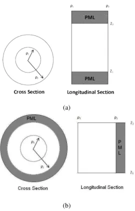
Fig. 2. Illustration of the geometry problem. (a) Longitudinal PML - (b) Radial PML

2) Geometric:

 

0

1

 

  

 

         

g (11a)







  

       

 

  

 1 2

ln 0 ln

0

  

  

d

g g

R (11b)

where 0



 is the CFS-PML conductivity at its surface, g is the scaling factor, and _ is the FV space

increment.

III. NUMERICAL RESULTS

A. Validation

In order to validate the present FV-CFS-PML method, the algorithm is applied to a lossless coaxial

waveguide backed by a cylindrical CFS-PML in both the longitudinal and radial directions, as illustrated

(a) (b)

Fig. 3. Electric field distribution of a lossless coaxial waveguide backed by a cylindrical CFS-PML. (a) Longitudinal PML - (b) Radial PML

following input data are used: the operating frequency is 2 MHz; both the relative electric

permittivity and magnetic permeability are set equal to 1; the inner cylinder has radius equal to r =

0.1016 m; the CFS-PML are set up using eight cells; max 4

10





 and the scaling factors are m=2 and

g=3.2. For the longitudinal PML case, the computational domain is discretized using a



N_,N_z



(50,300) grid.

The discretization cell size is uniform in both directions with _2.2m and z 5.0m. The source

is set at



N_,N_z



(10,150) and the field is sampled at 85.1m. For the radial PML case, a



N_,N_z



(100,80) grid is used. The discretization cell size is uniform in both directions with _5.0m and

m

z 1.5

 . The source is set at



N_,N_z



(51,35)and the field is sampled at 60.0m.

In fig. 3, the electric field distribution from the FV-PML simulation is compared against an

analytical solution. Very good agreement is observed between the FV-PML and analytical results.

This occurs because max



 is selected within the range defined by _max _0

  . Outside this range, the

CFS-PML does not exhibit induced attenuation.

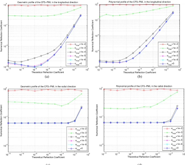
To better analyze the performance of the polynomial and geometric CFS-PML loss profiles, the

numerical (actual) coefficient reflection (COEFN) as a function of the theoretical coefficient

reflection (COEF) is plotted in Fig. 4,

for different values of

max





.

For the longitudinal CFS-PML

case, it can be noted that the polynomial-graded profile provides smaller reflection levels, showing an

advantage over the geometric-graded profile. However, max

z

 does not have strong influence on the

reflection level in both profiles. On the other hand, the COEFN does not vary with max



 in both

profiles for radial CFS-PML. Moreover, polynomial and geometric profiles provide similar reflection

levels. As expected, it can also be noted that for max ₀

(a) (b)

(c) (d)

Fig. 4. Numerical Reflection Coefficient X Theoretical reflection coefficient for different values of max



 . In bothprofiles, NPML=6 and KPML=1.

attenuation. It should be noted that the design of an effective CFS-PML requires balancing the

theoretical reflection error and the numerical discretization error. Normally, the CFS-PML

conductivity profile is chosen as large as possible to minimize the theoretical reflection error.

Unfortunately, if the CFS-PML conductivity profile is too large, the discretization error due to the FV

approximation dominates, and the numerical (actual) reflection error is potentially orders of

magnitude higher than what equation (10c) predicts. This problem is more pronounced in our case

because the cell size is too small.

Fig. 5 shows the COEFN as a function of max



 for different values of KPML (the real part of the

stretching variable s_). For the longitudinal CFS-PML case, it is observed that both profiles show

similar behavior, and the polynomial CFS-PML outperforms the geometric one. Note that for

4 max

10



z

 , COEFN has considerably increased in both profiles and for max 4

10



z

 , a slight variation is

observed in the geometric profile. However, for the radial CFS-PML case, it can be noted that

(a) (b)

(c) (d)

Fig. 5. Numerical Reflection Coefficient X max



 for different values of KPML. In both profiles, NPML=6.

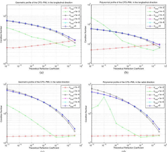
To investigate the impact of CFS-PML parameters on the condition number (CN) of the FV system

matrix, some of the input data have their values modified. In this study, the computational domain is

discretized using a



N_,N_z



(50,50) grid and the source is set at



N_,N_z



(25,25). The discretization cell size is uniform in both directions. For the longitudinal PML case, the domain was discretized by

using 2.2m and z 7.5m; and for the radial PML case, 2.2m and z 7.5m was used. Fig. 6

shows the CN as a function of COEF for different

values of

max





.

For both the longitudinal and the

radial CFS-PML case, it is observed that for max 4

10





 the CN decays as the COEF increases.

Moreover, it can be noted that both profiles (polynomial and geometric) show similar behavior. Fig. 7

shows the CN as a function of max



 for different values of KPML. Note that for max 4

10





 , the KPML

(a) (b)

(c) (d)

Fig. 6. Condition Number X Theoretical Reflection Coefficientfor different values of max



 . In both profiles, NPML=6 and KPML=1.

IV. CONCLUSION

We have compared the performance of two cylindrical CFS-PML, viz., polynomial-graded CFS-PML

and geometric-graded CFS-PML for being used as an absorbing boundary condition (ABC) in the

bi-dimensional (2-D) finite-volume technique in the frequency domain. Simulations in both the

longitudinal and radial coaxial waveguide terminated by a cylindrical CFS-PML have been carried

out. For the longitudinal CFS-PML case, the polynomial-graded CFS-PML has outperformed

geometric-graded PML in terms of wave absorption. However, the condition number of the associated

matrix system in both profiles are similar. For the radial CFS-PML case, both types of CFS-PML

have shown similar performance in terms of absorption of the wave, as well as the condition number

of the matrix system. Even though the CFS-PML has achieved great success in time-domain analysis,

(a) (b)

(c) (d)

Fig. 7. Condition Number X max



 for different values of KPML. In both profiles, NPML=6.

computational domain significantly increases the condition number of the system matrix and

consequently the convergence of iterative methods deteriorates.

REFERENCES

[1] A. Taflove and S. Hagness, Computational Eletrodynamics: The Finite-Difference Time-Domain Method, Boston MS: Artech House, 2005.

[2] U. Pekel and R. Mittra, A finite element method frequency-domain application of the perfectly matched layer (PML)

concept, Microwave Opt. Technol. Lett., vol. 9, pp.117 -122, 1995.

[3] Y. Y. Botros and J. L. Volakis, Preconditioned generalized minimal residual iterative scheme for perfectly matched

layer terminated applications, IEEE Micro. and Guide Wave Lett., vol. 9, no.2, Feb. 1999.

[4] D. Pardo, L. Demkowicz, C. Torres-Verdin, and C. Michler, PML Enhanced With A Self-Adaptive Goal-Oriented

pp-Finite Element Method: Simulation Of Through-Casing Borehole Resistivity Measurements, Siam Journal on Scientific

Computing, vol 30, no. 6, pp. 2948-2964, 2008.

[5] H. O. Lee, F. L. Teixeira, L. E. San Martin, and M. S. Bittar, Numerical modeling of eccentered LWD borehole sensors

in dipping and fully anisotropic Earth formations, IEEE Trans. Geosci. Remote Sens., vol. 50, no. 3, pp. 727-735, 2012.

[6] J. M. Jin and W.C. Chew, Combining PML and ABC for Finite Element Analysis of Scattering Problems, Micro. and Opt. Tech. Lett., vol. 12, no. 4, pp. 192-197, Jul. 1996.

[7] Y. Y. Botros and J. L. Volakis, Perfectly Matched Layer Termination for Finite-Element Meshes: Implementation and

Anisotropic Media With Multiple Horizontal Beds, IEEE Trans. Geoscience Remote Sens., vol.45, no.8, pp.2451-2462, 2007.

[11]M. S. Novo, L. C. da Silva and F. L. Teixeira, Finite Volume Modeling of Borehole Electromagnetic Logging in 3-D

Anisotropic Formations Using Coupled Scalar-Vector potentials, IEEE Antennas Wireless Propag. Lett., vol. 6, pp.

549-552, 2007.

[12]M. S. Novo, L. C. da Silva and F. L. Teixeira, Comparison of Coupledpotentials and Field-Based Finite-Volume

Techniques for Modeling of Borehole EM Tools, IEEE Geosci. Remote Sens. Lett., vol. 5, pp. 209-211, 2008.

[13]M. S. Novo, L. C. da Silva and F. L. Teixeira, Three-Dimensional Finite-Volume Analysis of Directional Resistivity

Logging Tools, IEEE Trans. Geosci. Remote Sens., vol. 48, pp. 1151-1158, Mar. 2010.

[14]M. S. Novo, L. C. da Silva and F. L. Teixeira, A Comparative Analysis of Krylov Solvers for Three-Dimensional Simulations of Borehole Sensors, IEEE Geosci. Remote Sens. Lett., vol. 8, no. 1, pp. 98-102, Jan. 2011.

[15]L. F. Ribeiro and M. S. Novo, Analysis of the Cylindrical PML ABC for 2-D Finite Volume Simulations in the

Frequency Domain, Proceedings of 2011 SBMO/IEEE MTT-S International Microwave and Optoelectronics

Conference, 2011, Natal.

[16]A. P. M. Lima and M. S. Novo, Analysis of Cylindrical CFS-PML ABC for 2-D Finite Volume Simulations in the

Frequency Domain, Proceedings of of 2013 SBMO/IEEE MTT-S International Microwave and Optoelectronics

Conference, 2013, Rio de Janeiro.

[17]M. Kuzuoglu and R. Mittra, “Frequency dependence of the constitutive parameters of causal perfectly matched

absorbers,” IEEE Microwave Guided Wave Lett., vol. 6, pp. 447–449, Dec. 1996.

[18]M. S. Novo, Análise numérica de sensores eletromagnéticos de prospecção petrolífera utilizando o método dos

volumes finitos, Pontifícia Universidade Católica do Rio de Janeiro, Departamento de Engenharia Elétrica, Tese de

Doutorado, Agosto 2007.

[19]F. L. Teixeira and W. C. Chew, Sistematic Derivation of Anisotropic PML Absorbing Media in Cylindrical and