Table 1 Maximum benefit duration before and after the reform

(1)

O R I G I N A L A R T I C L E

Open Access

Can a search model predict the effects of

an increase in the benefit duration? Evidence

from the Portuguese unemployment

insurance reform

Álvaro A. Novo

1

_{and André C. Silva}

2*

*Correspondence: andre.silva@novasbe.pt 2_{Nova School of Business and} Economics, Universidade Nova de Lisboa, Campus de Campolide, 1099-032 Lisbon, Portugal Full list of author information is available at the end of the article

Abstract

We test the predictions of an equilibrium search model about the effects of an increase in the maximum duration of unemployment benefits. We use the 1999 unemployment insurance reform of Portugal, a quasi-natural experiment. The reform increased the maximum duration of benefits for three groups of agents and maintained all features of the unemployment insurance for two other groups. We isolate the effects of the increase in the maximum duration of benefits and test the model. The model successfully predicts the effects on the unemployment rate, the labor force participation, and the levels of unemployment and employment.

JEL Classification: E24, J23, J64

Keywords: Unemployment duration, Unemployment benefits, Equilibrium search, Labor market reforms, Quasi-natural experiment

1 Introduction

In 1999, the Portuguese government increased the maximum duration of unemploy-ment benefits for workers with specific ages. We use this event to test if an equilibrium search model correctly predicts the effects of an increase in the maximum duration of unemployment benefits.

We use the model of Alvarez and Veracierto (2000), a general equilibrium search model for which the unemployment insurance system is modeled through the replacement ratio, the criteria of eligibility, and the duration of unemployment benefits. We test the model to determine to what extent a policy maker can use the model to make predictions about changes in the unemployment insurance system. Following the argument in Lucas (1981), once the model reproduces the effects of simpler policies, we have more confidence in its predictions about more complex policy changes.

The 1999 reform is a quasi-natural experiment as it created treatment and control groups in a way that resembles a controlled experiment. We first estimate the impact of the increase in the maximum benefit duration, following the literature on the effects of the unemployment insurance system on the labor market. We then use our results to test the search model.

(2)

Novo and SilvaIZA Journal of Labor Policy (2017) 6:3 Page 2 of 14

We find that the model is successful in predicting the effects on the unemployment rate, the labor force participation, and the levels of unemployment and employment. On the other hand, the average duration of unemployment decreased for the groups 15–24 and 40–44, while, as standard in search models, the model predicts an increase in the average duration of unemployment. In any case, the predictions lie within the confidence intervals for the estimates of the effects after the reform. For the group 30–34, the model correctly predicts the increase in the average duration of unemployment. In general, the differences between data and predictions are small.

2 The reform of the unemployment insurance system

The 1999 reform increased the maximum benefit duration for particular groups of agents. There were no changes in other aspects of the unemployment insurance system, such as the value of the benefit and the eligibility criterion. Before July 1999, there were eight maximum benefit durations. After July 1999, the number of maximum benefit durations decreased to four. The benefit duration is based only on the age of the recipient at the beginning of the unemployment spell. Table 1 summarizes the reform. The age groups 15–24, 30–34, and 40–44 are especially relevant for us, as these groups had an increase in the maximum benefit duration and each one has a well-defined control group.

The groups 15–24 and 25–29 form the first set of treatment and control groups, respectively. The maximum benefit duration of the group 15–24 increased from 10 to 12 months, which equalized the maximum benefit duration of the group 25–29. Simi-larly, the groups 30–34 and 35–39 form our second set of treatment and control groups, respectively. For the group 40–44, the maximum benefit duration increased from 21 to 24 months. As the maximum benefit duration of the next older age group, the group 45–49, also increased, we use the group 35–39 as control group for the group 40–44.

For the groups of agents older than 45, the maximum benefit duration became a func-tion of the number of years of social security contribufunc-tions. The dataset does not have the complete record of social contributions, and so, we cannot determine the increase in the maximum benefit duration. For the group 55–64, the reform introduced early retire-ment after a period of unemployretire-ment with little or no penalties. Early retireretire-ment affects agents in different ways than the increase in the maximum duration of benefits. For these reasons, we concentrate our analysis on the groups 15–24, 30–34, and 40–44. For these groups, we can determine the increase in the maximum benefit duration, and this was

Table 1Maximum benefit duration before and after the reform

Age Before (months) Age After (months) Change (months)

15–24 10 15–24 12 2

25–29 12 25–29 12 0

30–34 15 30–34 18 3

35–39 18 35–39 18 0

40–44 21 40–44 24 3

45–49 24 45–49 30 (+8)a _{6 (+8)}

50–54 27 50–54 30 (+8)a _{3 (+8)}

55–64 30 55–64 30 (+8)a _{0 (+8)}

Age at the beginning of the unemployment spell

(3)

the only change of the reform. The reform increased considerably the maximum benefit duration. The size of the increase helps the identification of the effects of the reform.

The good conditions around the time of the reform indicate that the reform was exoge-nous. The average real GDP growth was 3.3%, and the unemployment rate was 4.7% from 1997 to 2002 (data fromInstituto Nacional de Estatistica). The effects of a reform may be overstated if the reform is induced by recessions (Lalive et al. 2006; Lalive and Zweimüller 2004). This is not the case of the 1999 reform. Moreover, the rules of the reform applied only to those entering unemployment after the reform. This feature allows us to use agents before and after the reform to control for macroeconomic effects and for unobserved heterogeneity among agents.

3 The impact of the reform

We use social security administrative data fromInstituto de Informatica e Estatistica da Seguranca Socialfor data on the recipients of benefits. The dataset has wages and the amount and duration of unemployment benefits of all spells of unemployment benefit recipients from 1998 to 2002. The recipients are followed from the moment in which they register until they leave the system. The before period corresponds to the spells initiated from January 1998 to June 1999. The after period corresponds to the spells initiated from July 1999 to December 2002.1

For data on nonrecipients of benefits, labor force participation, and other labor statis-tics, we use the quarterly labor force surveyInquerito ao Emprego, fromInstituto Nacional de Estatistica. We use data from 1998:Q1 to 2002:Q4. We track transitions from inactivity, unemployment, and employment and compute the duration of unemployment spells. We have a total of 130,788 observations. From these, 104,686 correspond to spells initiated after the reform. Table 2 shows summary statistics by age group.

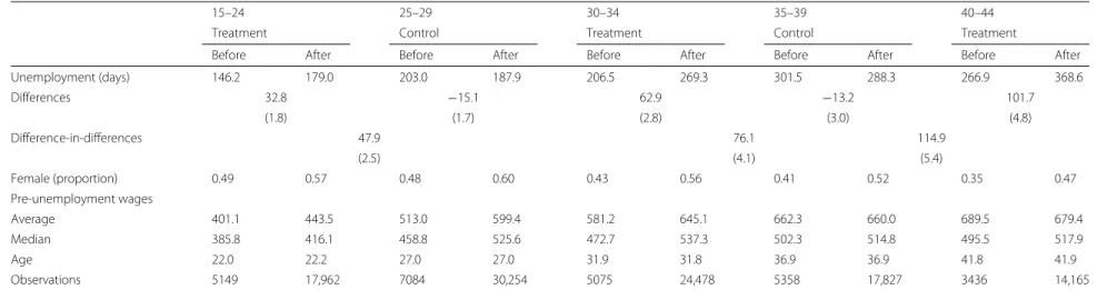
The proportion of males and females across treatment and control groups is similar. It varies from 41 to 60% for women, with the exception of the 40–44 group before the reform, with 35%. There are larger differences in ages and pre-unemployment wages. The effect of age is the result of the definition of the treatment and control groups, which yields older control units. Similarly, pre-unemployment wages are higher for older agents, which is expected given the age and tenure profile of wages. The inclusion of age in the conditional difference-in-differences estimator, as done below, corrects for the observed heterogeneity.

The average treatment impacts on the duration of unemployment of benefit recipi-ents are 48, 76, and 115 days for the 15–24, 30–34, and 40–44 age groups, respectively (Table 2). All estimates are statistically and economically significant. The impact reflects the decisions of agents to increase the duration of their search as unemployed work-ers. They could have opted for not using the increased generosity and even reduce their unemployment spells, as it occurred for the two control groups.

(4)

Novo

and

Silva

IZA

Journal

of

Labor

Policy

(2017) 6:3

Page

4

of

14

Table 2Summary statistics and unconditional difference-in-differences

15–24 25–29 30–34 35–39 40–44

Treatment Control Treatment Control Treatment

Before After Before After Before After Before After Before After

Unemployment (days) 146.2 179.0 203.0 187.9 206.5 269.3 301.5 288.3 266.9 368.6

Differences 32.8 −15.1 62.9 −13.2 101.7

(1.8) (1.7) (2.8) (3.0) (4.8)

Difference-in-differences 47.9 76.1 114.9

(2.5) (4.1) (5.4)

Female (proportion) 0.49 0.57 0.48 0.60 0.43 0.56 0.41 0.52 0.35 0.47

Pre-unemployment wages

Average 401.1 443.5 513.0 599.4 581.2 645.1 662.3 660.0 689.5 679.4

Median 385.8 416.1 458.8 525.6 472.7 537.3 502.3 514.8 495.5 517.9

Age 22.0 22.2 27.0 27.0 31.9 31.8 36.9 36.9 41.8 41.9

Observations 5149 17,962 7084 30,254 5075 24,478 5358 17,827 3436 14,165

(5)

indicator is the reduction in the unemployment duration of only 2 weeks for the control groups.

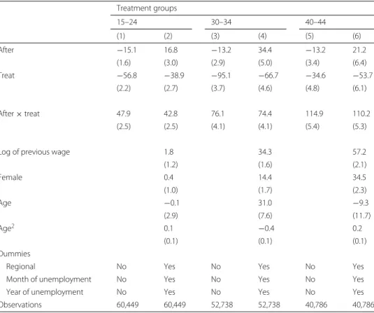
Table 3 shows the difference-in-differences estimates of the impact of the increase in the maximum benefit duration on the duration of unemployment for benefit recipients. The introduction of control variables yields a slightly lower impact: from 48 to 43 days for the group 15–24, 76 to 74 days for the group 30–34, and 115 to 110 days for the group 40–44. The size of the estimates is consistent with estimates obtained for Portugal and for other countries. For Portugal, Addison and Portugal (2008) find a large elasticity of the unem-ployed workers to the benefit duration. Using survey data, they obtain that an increase in the benefit duration of 3 months reduces the escape rate by 70%. Pereira (2006) finds that an increase in the maximum benefit period decreases the probability of leaving unem-ployment with benefits. Our results are also consistent with Centeno and Novo (2007), although they use the nonparametric Kaplan-Meyer estimator and the quantile treatment effect method.

For Slovenia, Van Ours and Vodopivec (2006) obtain a large impact on unemployment duration for a reduction in the benefit duration. They find that the cumulative probabil-ity of leaving unemployment after 12 months increases from 63 to 77% when the benefit duration is reduced from 12 to 6 months. For Germany, Hunt (1995) obtains a reduc-tion of 46% in the hazard of unemployment for an increase in the durareduc-tion of benefits of 6 months.2

Table 3The impact of the reform, difference-in-differences estimates (in days) Treatment groups

15–24 30–34 40–44

(1) (2) (3) (4) (5) (6)

After −15.1 16.8 −13.2 34.4 −13.2 21.2

(1.6) (3.0) (2.9) (5.0) (3.4) (6.4)

Treat −56.8 −38.9 −95.1 −66.7 −34.6 −53.7

(2.2) (2.7) (3.7) (4.6) (4.8) (6.1)

After×treat 47.9 42.8 76.1 74.4 114.9 110.2

(2.5) (2.5) (4.1) (4.1) (5.4) (5.3)

Log of previous wage 1.8 34.3 57.2

(1.2) (1.6) (2.1)

Female 0.4 14.4 34.5

(1.0) (1.7) (2.3)

Age −0.1 31.0 −9.3

(2.9) (7.6) (11.7)

Age2 _0.1 ₋_0.4 _0.2

(0.1) (0.1) (0.1)

Dummies

Regional No Yes No Yes No Yes

Month of unemployment No Yes No Yes No Yes

Year of unemployment No Yes No Yes No Yes

Observations 60,449 60,449 52,738 52,738 40,786 40,786

The group 25–29 is the control group for the treatment group 15–24. The group 35–39 is the control group for the treatment groups 30–34 and 40–44. Age at the beginning of the subsidized period. The coefficient onAfter×treatis the

(6)

4 Can a search model predict the effects of the reform?

We use the model of Alvarez and Veracierto (2000) because it considers separately the duration of unemployment benefits, the replacement rate, and the eligibility criterion. Moreover, the labor force is endogenous in the model. We can then change the duration of benefits and calculate the effects on labor market variables, including the labor force.3 There are different production sectors. Productivity in each sector changes over time. The agents decide to stay, move to another sector, or leave the labor market according to the productivity. If the agents move, they search for one period as unemployed workers and are assigned randomly to another sector in the following period. If they leave the labor market, they engage in home production. Agents in home production have to search for one period to reenter the labor market.

Agents have preferences

E0

∞

t=0

βt

c1_t−γ−1 1−γ +ht

, (1)

wherectis consumption of market goods,htis consumption of home goods, 0< β <1,

andγ ≥0. Higherγ implies that it is more difficult to substitute home goods for market goods. Production of market goods in each sector is given byyt=ztgαt, 0< α <1, where gtis the number of employed agents andztis the productivity of the sector. Productivity

follows logzt+1=ρlogzt+εt+1, whereεt+1has normal distribution with mean zero and varianceσ2, independent across sectors, 0 < ρ < 1. Each sector begins withxagents. Some of these agents work and others leave, sog(x,z) ≤ x. LetU, to be determined in equilibrium, denote the number of agents that arrive in each sector in every period as unemployed agents. The number of agents in the sector(x,z)in the following period is

x′=g(x,z)+U.

Agents that stay in a certain sector receive wagesw(x,z)and begin the following period in the same sector as workers. Wages are equal to the marginal productivity of labor. The value of being in sector(x,z), so far without unemployment insurance, is

v(x,z)=max w

g(x,z),z +βE

v

g(x,z)+U,z′ |z ,θ

, (2)

whereθis the value of the search. Home production yieldswhgoods. Asθis the value of an agent who leaves a sector, it satisfies

θ =maxβE[v(x,z)] ,wh+βθ; (3)

θ is equal to the maximum between the values of staying in the labor force as an unemployed worker,βE[v(x,z)], and leaving the labor force,wh₊_βθ_.

The equilibrium conditions are the following. First, agents outside the labor force are indifferent between searching or staying out of the labor force; therefore,βE[v(x,z;U)]= wh+βθ. Second, the value of leaving a sector is equal to the present value of home pro-duction. This condition impliesθ = wh/ (1−β)whenγ = 0 andθc−γ ₌ _wh_{/ (}₁₋_β)

whenγ >0, wherecis the aggregate consumption of the market good.

(7)

with lump-sum taxes. The increase in the maximum duration of benefits is modeled as an increase inψ.

The value of the search for ineligible agents,θ0, and eligible agents,θ1, are given by

θ0 = max

wh+βθ0,βE[max{v(x,z),θ0}]

, (4)

θ1 = b+max

wh+β[ψ θ1+(1−ψ ) θ0] ,

β (ψE[max{v(x,z),θ1}]+(1−ψ )E[max{v(x,z),θ0}])

.

The agents take into account that they will be eligible in the following period with prob-abilityψ. The value of beginning in sector(x,z)for a worker employed in the previous period changes to

v(x,z)=max w

g(x,z),z +βE

v

g(x,z)+U,z′

|z ,κθ₁+(1−κ) θ₀

. (5)

The value of the search,κθ1+(1−κ) θ0, now depends on the probability of eligibility. The equilibrium conditions are similar to the case without unemployment insurance, with the different functional form ofv(x,z)and the additional conditions forθ0andθ1. The unemployment insurance system increases the value of work, which increases the labor force participation and the average duration of unemployment.

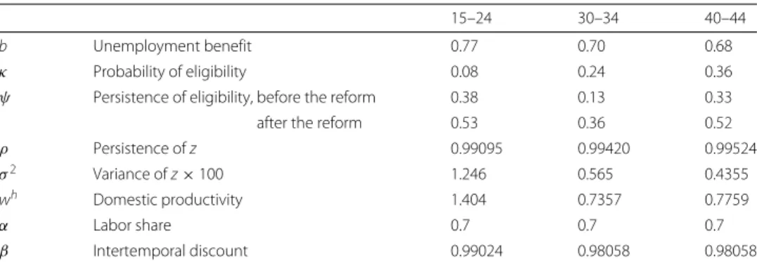
To obtain the parameters (Table 4), we follow Alvarez and Veracierto (2000, 2001), Gomes et al. (2001), Ljungqvist and Sargent (2007), and, for Portuguese data, Cavalcanti (2007) and Silva (2008). The three critical parameters of the model areb,ψ, andκ, which characterize the unemployment insurance system.

Given the heterogeneity of the groups, we obtain the parameters for each group sep-arately. The groups are 10 to 25 years apart and in different positions of their life cycle. The unemployment rate of the group 40–44 before the reform, for example, was 3.8%, less than half the unemployment rate of 10% of the group 15–24. The ratio of recipients to unemployed workers was 8% for the group 15–24, 24% for the group 30–34, and 36% for the group 40–44.

We set the unemployment benefitbfrom the average replacement ratio in the period before the reform (1998:Q1 to 1999:Q2). In contrast to the structure in the USA, there are no experience-rated taxes or other taxes that mix unemployment benefits with firing costs (Anderson and Meyer 2000). For the probability of eligibilityκ, we use the ratio of recipients to unemployed workers. As the reform did not change the eligibility criterion, we setκ equal to the average ratios before and after the reform. For the 30–34 group,

Table 4Parameters

15–24 30–34 40–44

b _{Unemployment benefit} _0.77 _0.70 _0.68

κ Probability of eligibility 0.08 0.24 0.36

ψ Persistence of eligibility, before the reform 0.38 0.13 0.33

after the reform 0.53 0.36 0.52

ρ Persistence ofz 0.99095 0.99420 0.99524

σ2 Variance ofz×100 1.246 0.565 0.4355

wh _{Domestic productivity} _1.404 _0.7357 _0.7759

α Labor share 0.7 0.7 0.7

β Intertemporal discount 0.99024 0.98058 0.98058

(8)

for example, the ratio before and after the reform increased from 23 to 25%. We use the average of the two values, 24%.

The probability of maintaining eligibilityψimplies that the expected duration of eligi-bility is 1/ (1−ψ )periods. As it is common in the literature, we use data on the average duration of unemployment benefits. For before the reform, we use the average duration from 1998:Q1 to 1999:Q2. For after the reform, we use the results from the controlled experiment obtained in Section 3. These results remove the effects unrelated to the reform. For the 30–34 group, for example, the average duration of benefits increased from 6.9 to 9.4 months. The duration of 9.4 months is obtained through the sum of the esti-mate in Table 3 to the unemployment duration of benefit recipients before the reform:

(206.5+74.4)/30=9.4 months. Using raw data alone mix the effects of the reform with the effects of the economic cycle. The values ofψfor before and after the reform are such that the expected duration of unemployment benefits is 6.9 months before and 9.4 months after the reform. Notice that Gomes et al. (2001) and Ljungqvist and Sargent (2007) do not have a value forψ, as the unemployment benefits in their models last for the whole duration of the unemployment spell.

For the labor share, we use Gollin (2002). He obtains three estimates for the labor share in Portugal: 0.602, 0.748, and 0.825, according to the calculation of the income of the self-employed. He setα = 0.7, a little smaller than the mean of the three estimates, as Gollin points out that the highest estimate can overstate the labor share.4_{We set home} productionwhso that the model matches the data on labor force participation before the reform.whonly affects labor force participation; it does not affect the unemployment rate or the duration of unemployment.

We setρ andσ2to match the average duration of unemployment and the unemploy-ment rate before the increase in the benefit duration. The labor market in Portugal shows high average duration of unemployment combined with a relatively low unemployment rate: for the group 30–34, the unemployment duration before the policy change was 24 months while the unemployment rate was 4.9%. Blanchard and Portugal (2001) analyze the combination of high average duration and low unemployment rate for Portugal. High unemployment duration and low unemployment rate demandsρclose to one. As a result, the productivity processzapproaches a random walk and the numerical algorithm can-not approximate precisely the theoretical distribution ofz. To circumvent this problem, we use a model period of 3 months for the 15–24 age group and 6 months for the groups 30–34 and 40–44. We use a smaller model period for the 15–24 group because the benefit duration for this group is 4.9 months, smaller than 6 months.

We set the intertemporal discountβso that it is equivalent to an interest rate of 4% per year. We considerγ =0, 1, 8.γ =0 implies perfect substitution, andγ =1 (logarithmic utility) implies that wages do not affect labor supply.γ =8 matches the evidence on the elasticity of the labor force with respect to a tax on labor (Alvarez and Veracierto 2000).

(9)

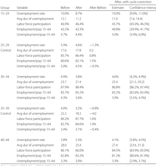
Table 5Treatment of the labor market variables for the economic cycle

After, with cycle correction

Group Variable Before After After-Before Estimate Confidence interval

15–24 Unemployment rate 10.0% 8.7% 10.0% [9.0%, 11.0%]

Avg dur of unemployment 12.1 11.2 11.0 [7.6, 14.4]

Labor force participation 46.9% 46.4% 45.7% [45.0%, 46.3%]

Employment/pop 15–64 42.2% 42.3% 40.8% [39.9%, 41.7%]

Unemployment/pop 15–64 4.7% 4.4% 5.0% [3.9%, 6.0%]

25–29 Unemployment rate 5.9% 4.6% −1.3%

Control Avg dur of unemployment 17.6 17.8 0.2 Labor force participation 85.7% 86.4% 0.8% Employment/pop 15–64 80.6% 82.1% 1.5% Unemployment/pop 15–64 5.0% 4.5% −0.5%

Employment/pop 15–64 83.7% 85.2% 83.2% [82.6%, 83.9%]

35–39 Unemployment rate 4.0% 3.2% −0.8%

Control Avg dur of unemployment 22.2 18.2 −4.0 Labor force participation 86.2% 87.7% 1.6% Employment/pop 15–64 82.7% 84.6% 1.9% Unemployment/pop 15–64 3.4% 3.1% −0.4%

Employment/pop 15–64 82.8% 83.2% 81.2% [80.6%, 81.9%]

Before: 1998:1–1999:2. After: 1999:3–2002:4. Confidence intervals with two standard deviations. Average duration of

unemployment in months. The values after correction for the cycle are obtained by subtracting the variation of the control group from the observed rate. For example: 10.0%=8.7%−(−1.3%)for the unemployment rate of the group 15–24

correction factors obtained from the control groups, and the estimated values after the correction along with their confidence intervals.

Consider the unemployment rate for the group 15–24, which decreased from 10.0 to 8.7%. For its control group, 25–29, the unemployment rate decreased from 5.9 to 4.6%. As the unemployment insurance system did not change for the group 25–29, we assign the decrease of 1.3 percentage points to changes unrelated to the reform. Correcting for these changes, the unemployment rate for the group 15–24 stays constant at 8.7−(−1.3) =

10.0%. We proceed in a similar way for the average duration of unemployment, the labor force participation, and the levels of employment and unemployment.

(10)

We use nonrecipients of unemployment benefits for the average duration of unemploy-ment as the average duration of unemployunemploy-ment in the model refers to unemployed agents without benefits (Alvarez and Veracierto 2000). A decrease in the search effort of eligible agents is compatible, for example, with the evidence in Lalive et al. (2005), who found a decrease in unemployment duration when the government increases the monitoring of benefit recipients.5

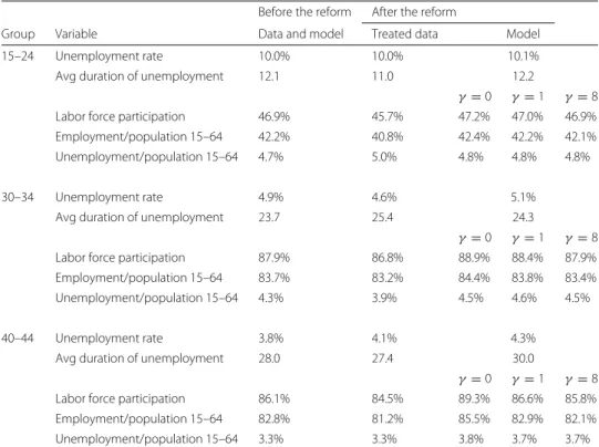
We confront predictions and data in Table 6 and in Fig. 1. Consider first the labor force, employment, and unemployment, the variables that depend on the substitution parame-terγ. In the data, the labor force participation and the level of employment decreased for all groups.6Moreover, the level of unemployment increases for the groups 15–24 and 40– 44 (it is approximately constant for the group 40–44). With low substitution,γ = 8, the model reproduces these facts: a decrease in the labor force, an increase in unemployment, and a decrease in employment after the increase in the maximum duration of benefits. The model withγ =8 has a better match to the data. For this choice ofγ, the predictions are on average 4% different from the data after the reform.

The model predicts an increase in the unemployment rate and in the average duration of unemployment when the maximum duration of benefits increase, as standard in search models. The data show approximately constant unemployment rate after the reform: from a decrease of 0.3% for the 30–34 group to an increase of 0.3% for the 40–44 group. The model better predicts the changes on the unemployment rate for the groups 15–24 and 40–44. The average duration of unemployment decreased for the groups 15–24 and 40–44 while it increased for the group 30–34. Therefore, the model better predicts the

Table 6Data and predictions of the model

Before the reform After the reform

Group Variable Data and model Treated data Model

15–24 Unemployment rate 10.0% 10.0% 10.1%

Avg duration of unemployment 12.1 11.0 12.2

γ=0 γ=1 γ=8

Labor force participation 46.9% 45.7% 47.2% 47.0% 46.9%

Employment/population 15–64 42.2% 40.8% 42.4% 42.2% 42.1%

Unemployment/population 15–64 4.7% 5.0% 4.8% 4.8% 4.8%

γ=0 γ=1 γ =8

(11)

Fig. 1Data and predictions.Arrows_{: model predictions,}_γ=8.Lines_{: data and confidence intervals with two}

standard deviations

average duration of unemployment for the group 30–34. For all groups, the predictions are within the confidence intervals for the estimated values after the reform.

For the group 30–34, the duration of unemployment increased from 23.7 to 25.4 months. The model predicts an increase to 24.3 months, 1 month below the data, an error of 4%. The unemployment rate decreased from 4.9 to 4.6% while the model predicts an increase to 5.1%, an upward error of 0.5 percentage points or 11%.

For the group 15–24, the model predicts small changes because only 8% of the unem-ployed workers in this group received benefits. The duration of unemployment decreased from 12.1 to 11.0 months while the model predicts an increase to 12.2 months. The unem-ployment rate stayed constant at 10.0% while the model predicts an increase to 10.1%. Apart from the labor force participation and the employment level, the predictions are within the confidence intervals for the values after the reform.

For the group 40–44, the duration of unemployment decreased from 28.0 to 27.4 months while the model predicts an increase to 30.0 months. Relatively to the data after the reform, it implies a difference of 2.6 months or 9%. The unemployment rate increased from 3.8 to 4.1%, and the model predicts an increase to 4.3%, a difference of 0.2 percentage points or 4%.

(12)

this group is small. Nevertheless, the predictions of the model are within the confidence intervals for all groups, as shown in Fig. 1.

The model does not have factors such as borrowing constraints, directed search, and ex ante heterogeneity of agents.7It is not a surprise to find that the model does not match the data in all cases. Moreover, part of the effects in the data may refer to a transitional period. To approximate the steady states, we follow the usual procedure of taking the average of a long period before and after the reform (see Van den Berg (1990) for an analysis of nonstationary job search models). In particular, for the period after, we take the average of more than 3 years after the reform.

The model gets closer to the data for the labor force participation, employment, and unemployment. For the labor force participation, the model correctly predicts the changes but the predictions for this variable are outside the confidence intervals. The model has a better match to the data forγ = 8. In this case, the model matches the direction of change of 9 out of 15 variables studied (five for each of the three groups). The model is able to predict satisfactorily the effects of the reform for the three age groups. When the model cannot predict the effects of the reform, the differences are usually small.

5 Conclusions

We identify a reform particularly appropriate to evaluate an equilibrium search model for the labor market. It is usually not possible to use a controlled experiment to evaluate a model. In rare cases, a change such as the 1999 reform resembles a controlled experiment. We show that an equilibrium search model is able to reproduce most of the effects of an increase in the maximum duration of unemployment benefits. The model predictions are close to the data on the unemployment rate, the labor force participation, and the levels of employment and unemployment.

General equilibrium models are useful for policy evaluation. As Meghir (2007) points out, these models can be used to predict long-run effects and to run counterfactuals. They complement empirical studies. However, we can only trust the predictions of a model if it reproduces the facts of policy changes for which we have alternative esti-mators of their impact. We conclude that the model reproduces the facts in various dimensions. This finding increases our confidence to expose the model to more complex changes.

Endnotes

1_{The dataset records subsidized unemployment duration, not the total duration of}

unemployment. However, as the maximum durations of benefit are large, the duration of a spell in the dataset is usually equal to the total duration of unemployment.

2_{Lalive et al. (2006) and Card et al. (2007) obtain smaller effects for Austria. Lalive}

et al. also obtain that, restricting the sample to narrower age groups, the estimates of the effects of extended benefits are three times larger than their baseline estimates.

3_{We describe the model briefly. The framework follows the search-island model of}

(13)

4_{Cavalcanti (2007) uses}_α ₌ _{0.56, not taking into account labor income of the}

self-employed. Silva (2008) usesα = 0.7. The conclusions of the paper do not change with such changes inα.

5_{We use the official unemployment rate, which includes recipients and nonrecipients}

and the average duration of nonrecipients. As the unemployment rates for all unemployed agents and for nonrecipients move in parallel (it is 1.3 percentage points above the rate for nonrecipients before and after the reform), our conclusions do not change if we use the unemployment rate for nonrecipients.

6_{Haan and Prowse (2010), with data for Germany, find that employment increases if}

the duration of benefits decreases.

7_{Alvarez and Shimer (2011) consider a search-island model with rest unemployment,}

when agents wait until the labor market conditions improve. See Rogerson et al. (2005) for a survey. Another aspect is the optimal unemployment insurance policy, analyzed, for example, in Coles and Masters (2006) and Shimer and Werning (2007).

Acknowledgements

The views in this paper are those of the authors and do not necessarily reflect the views of the Banco de Portugal. We thank Pedro Amaral, António Antunes, Mário Centeno, Brian McCall, Marcelo Veracierto, Till von Wachter, and participants in seminars and conferences for valuable comments and discussions. Silva thanks the hospitality of the Banco de Portugal, where he wrote part of this paper, and acknowledges financial support from Banco de Portugal, FCT, NOVA FORUM, and Nova SBE Research Unit. This work was funded by National Funds through FCT-Fundação para a Ciência e Tecnologia under the projects Ref. FCT PTDC/IIM-ECO/4825/2012 and Ref. UID/ECO/00124/2013 and by POR Lisboa under the project LISBOA-01-0145-FEDER-007722. We would also like to thank the anonymous referee and the editor for the useful remarks. Responsible editor: Juan Jimeno

Competing interests

The IZA Journal of Labor Policy is committed to the IZA Guiding Principles of Research Integrity. The authors declare that they have observed these principles.

Publisher’s Note

Springer Nature remains neutral with regard to jurisdictional claims in published maps and institutional affiliations. Author details

1_{Banco de Portugal, Av. Almirante Reis 71, DEE, 1150-021 Lisbon, Portugal.}2_{Nova School of Business and Economics,} Universidade Nova de Lisboa, Campus de Campolide, 1099-032 Lisbon, Portugal.

Received: 17 May 2016 Accepted: 4 March 2017

References

Addison JT, Portugal P (2008) How do different entitlements to unemployment benefits affect the transitions from unemployment into employment? Econ Lett 101(3):206–209

Alvarez F, Shimer R (2011) Search and rest unemployment. Econometrica 79(1):75–12

Alvarez F, Veracierto M (2000) Labor market policies in an equilibrium search model. In: Bernanke BS, Rotemberg JJ (eds) NBER Macroeconomics Annual 1999. MIT Press, Cambridge, MA Vol. 14. pp 265–304

Alvarez F, Veracierto M (2001) Severance payments in an economy with frictions. J Monet Econ 47:477–498

Anderson PM, Meyer BD (2000) The effects of the unemployment insurance payroll tax on wages, employment, claims and denials. J Public Econ 78:81–106

Blanchard O, Portugal P (2001) What hides behind an unemployment rate: comparing Portuguese and U.S. labor markets. Am Econ Rev 91(1):187–207

Card D, Chetty R, Weber A (2007) Cash-on-hand and competing models of intertemporal behavior: new evidence from the labor market. Q J Econ 122(4):1511–1560

Cavalcanti TV (2007) Business cycle and level accounting: the case of Portugal. Port Econ J 6(1):47–64

Centeno M, Novo AA (2007) Identifying unemployment insurance income effects with a quasi-natural experiment. Banco de Portugal, Working Paper 2007–10

Cole HL, Rogerson R (1999) Can the Mortensen-Pissarides matching model match the business cycle facts? Int Econ Rev 40:933–959

Coles M, Masters A (2006) Optimal unemployment insurance in a matching equilibrium. J Labor Econ 24(1):109–138 Gollin D (2002) Getting income shares right. J Polit Econ 110(21):458–474

Gomes J, Greenwood J, Rebelo S (2001) Equilibrium unemployment. J Monet Econ 48:109–152

(14)

Hunt J (1995) The effect of unemployment compensation on unemployment duration in Germany. J Labor Econ 13(1):88–120

Lalive R, van Ours J, Zweimüller J (2005) The effect of benefit sanctions on the duration of unemployment. J Eur Econ Assoc 3(6):1386–1417

Lalive R, van Ours J, Zweimüller J (2006) How changes in financial incentives affect the duration of unemployment. Rev Econ Stat 73(4):1009–1038

Lalive R, Zweimüller J (2004) Benefit entitlement and unemployment duration: the role of policy endogeneity. J Public Econ 88(12):2587–2616

Ljungqvist L, Sargent TJ (2007) Understanding European unemployment with matching and search-island models. J Monet Econ 54:2139–2179

Lucas RE (1981) Methods and problems in business cycle theory. In: Studies in Business Cycle Theory. MIT Press, Cambridge, MA

Lucas RE, Prescott EC (1974) Equilibrium search and unemployment. J Econ Theory 7(2):188–209

Meghir C (2007) Dynamic models for policy evaluation. In: Blundell R, Newey W, Persson T (eds). Advances in economics and econometrics: theory and applications, ninth world congress, vol II. Cambridge University Press, Cambridge. pp 255–278

Mortensen DT, Pissarides CA (1994) Job creation and job destruction in the theory of unemployment. Rev Econ Stud 61:397–415

Pereira A (2006) Assessment of the changes in the Portuguese unemployment insurance system. Banco de Portugal Econ Bull 12(1):51–65

Rogerson R, Shimer R, Wright R (2005) Search-theoretic models of the labor market: a survey. J Econ Lit 43(4):959–988 Shimer R, Werning I (2007) Reservation wages and unemployment insurance. Q J Econ 122(3):1145–1185

Silva AC (2008) Taxes and labor supply: Portugal, Europe, and the United States. Port Econ J 7(2):101–124 Van den Berg GJ (1990) Nonstationarity in job search theory. Rev Econ Stud 57(2):255–277

Van Ours JC, Vodopivec M (2006) How shortening the potential duration of unemployment benefits affects the duration of unemployment: evidence from a natural experiment. J Labor Econ 24(2):351–377

Submit your manuscript to a

journal and beneﬁ t from:

7Convenient online submission

7Rigorous peer review

7Immediate publication on acceptance

7Open access: articles freely available online

7High visibility within the fi eld

7Retaining the copyright to your article