www.atmos-chem-phys.net/16/14979/2016/ doi:10.5194/acp-16-14979-2016
© Author(s) 2016. CC Attribution 3.0 License.
Gridded uncertainty in fossil fuel carbon dioxide
emission maps, a CDIAC example
Robert J. Andres1, Thomas A. Boden1, and David M. Higdon2
1Carbon Dioxide Information Analysis Center, Oak Ridge National Laboratory, Oak Ridge, TN 37831-6290, USA 2Biocomplexity Institute, Virginia Tech University, Blacksburg, VA 24061-0477, USA
Correspondence to:Robert J. Andres ([email protected])
Received: 23 March 2016 – Published in Atmos. Chem. Phys. Discuss.: 13 April 2016 Revised: 22 September 2016 – Accepted: 13 November 2016 – Published: 5 December 2016
Abstract. Due to a current lack of physical measurements at appropriate spatial and temporal scales, all current global maps and distributions of fossil fuel carbon dioxide (FFCO2) emissions use one or more proxies to distribute those emis-sions. These proxies and distribution schemes introduce ad-ditional uncertainty into these maps. This paper examines the uncertainty associated with the magnitude of gridded FFCO2 emissions. This uncertainty is gridded at the same spatial and temporal scales as the mass magnitude maps. This gridded uncertainty includes uncertainty contributions from the spa-tial, temporal, proxy, and magnitude components used to cre-ate the magnitude map of FFCO2 emissions. Throughout this process, when assumptions had to be made or expert judg-ment employed, the general tendency in most cases was to-ward overestimating or increasing the magnitude of uncer-tainty. The results of the uncertainty analysis reveal a range of 4–190 %, with an average of 120 % (2σ) for populated and FFCO2-emitting grid spaces over annual timescales. This pa-per also describes a methodological change specific to the creation of the Carbon Dioxide Information Analysis Center (CDIAC) FFCO2 emission maps: the change from a tempo-rally fixed population proxy to a tempotempo-rally varying popula-tion proxy.
Copyright statement
This paper was written by UT-Battelle, LLC under Contract no. DE-AC05-00OR22725 with the US Department of En-ergy. The United States Government retains and the pub-lisher, by accepting the article for publication, acknowledges that the United States Government retains a non-exclusive,
paid-up, irrevocable, world-wide license to publish or re-produce the published form of this paper, or allow others to do so, for United States Government purposes. The De-partment of Energy will provide public access to these re-sults of federally sponsored research in accordance with the DOE Public Access Plan (http://energy.gov/downloads/ doe-public-access-plan).
1 Introduction
uncer-tainty: (1) in terms of absolute mass, the mass of uncertain emissions is increasing with time as the total FFCO2 flux is increasing with time (assuming a constant percentage tainty), and (2) in terms of relative mass, the percent uncer-tainty is increasing with time as more FFCO2 emissions are coming from nations with less certain emissions.
Even with the improvements mentioned above, it is not presently possible to directly measure any one component of the global carbon cycle completely and exclusively at signif-icant spatial and temporal scales. Due to process interplay and mixing, direct samples carry the history of global car-bon cycle processes within them and oftentimes models are used to deconvolve the effects of these processes on the sam-ple data. This process can lead to a better understanding of the global carbon cycle. One approach to increase knowledge of the global carbon cycle is to sample at finer spatial and temporal scales to better isolate specific components of the global carbon cycle.
This paper examines the FFCO2 component of the global carbon cycle after it is parsed into a grid. Such gridded FFCO2 data are often incorporated into global carbon cy-cle and global climate (and/or Earth system) models to better understand the interplay amongst various components. Par-alleling early efforts in global carbon cycle science where the majority of the effort was concentrated on better esti-mating the component magnitudes (e.g., FFCO2, land use, atmospheric growth, oceanic uptake, and the terrestrial bio-sphere), present efforts in gridding FFCO2 emissions are also concentrated on better estimating the flux in each grid cell. These gridding efforts are not trivial in terms of time and data required. Robust estimates of the uncertainty associated with gridded FFCO2 estimates should have at least two ma-jor effects: (1) better evaluation of different FFCO2 gridding methodologies to assess whether they give statistically dif-ferent distributions, and (2) more importantly, allow for fur-ther advances in the collective community understanding of global carbon cycle processes, their interplay, and a charac-terization of change over space and time.
The transfer of carbon from one reservoir to another over a given time interval can be called a carbon flux. In this paper, the carbon flux from the fossil fuel reservoir to the atmo-spheric reservoir through the processes of combustion will be examined. More specifically, this paper will pursue a sys-tematic uncertainty analysis that applies to the carbon flux gridded mass data products (i.e., maps) presented by Andres et al. (1996), but also could be applied to other maps such as those produced by Olivier et al. (2005, EDGAR), Gur-ney et al. (2009, VULCAN), Rayner et al. (2010, FFDAS), Oda and Maksyutov (2011, ODIAC), and Wang et al. (2013, PKU-CO2). This paper does not describe production of un-certainty maps for other distribution methodologies, as the creators of those methodologies are in the best informed po-sition to create such maps. Also, this paper does not compare the gridded FFCO2 mass maps of Andres et al. (1996) to these other maps.
All of these map products attempt to capture the transfer of carbon from the fossil hydrocarbon reservoir to the atmo-spheric reservoir at varying degrees of spatial and temporal resolution. Each of these map products incorporates differ-ent features (i.e., data and schemes) to map FFCO2 emis-sions in space and time. Since very few measurements exist to accurately plot FFCO2 emissions in space and time, all of these map products utilize various proxies to locate FFCO2 emissions on a two-dimensional surface (i.e., a map) for a given time interval (e.g., a year). These proxies may include population distributions, power plant locations, road and rail networks, traffic counts, nighttime lights, etc..
This uncertainty analysis does not apply to maps such as those produced using satellite observations (e.g., GOSAT (http://www.gosat.nies.go.jp) or OCO-2 (http://oco.jpl.nasa. gov/)). Satellites measure burdens (which can lead to the con-centration of carbon) in the atmosphere that are fundamen-tally an estimate of the size of a reservoir (i.e., mass of carbon in the reservoir). Of course, taking the difference between two such maps could lead to an estimate of the carbon flux. While portions of the uncertainty analysis presented herein could be applied to such maps, this paper will not focus on uncertainty analysis for maps derived from satellite data.
The Carbon Dioxide Information Analysis Center (CDIAC), Oak Ridge National Laboratory (ORNL), United States (US), FFCO2 time series (Boden et al., 2015) gives an estimate of FFCO2 emissions from all nations in the world at annual time steps using the fundamental methods of Marland and Rotty (1984). The FFCO2 time series is updated periodically with each update adding another year to the time series as well as revising data in previous years. Over the years, new dimensions to this basic time series have been produced, including mapping the emissions at 1◦latitude by 1◦longitude (Andres et al., 1996), extending the time series back to the year 1751 (Andres et al., 1999), describing the time series in terms of stable carbon isotopic (δ13C) signature (Andres et al., 2000), parsing the time series from annual to monthly time steps (Andres et al., 2011), and describing the uncertainty of the total global FFCO2 emissions (Andres et al., 2014). With the global FFCO2 emission uncertainty analysis completed, a gridded uncertainty analysis can be applied to the annual and monthly maps. This uncertainty analysis will be applied to the mass maps only. Application to the stable carbon isotopic signature maps (i.e., annual and monthly) will need to wait until a separate uncertainty analysis of theδ13C signatures is completed.
the gridded uncertainty maps can also be updated and ex-tended. The initial year of the gridded uncertainty maps is limited by the beginning of the global uncertainty analysis, which begins with the year 1950.
As was done with the global uncertainty estimates (An-dres et al., 2014), 2σ uncertainties will be used throughout this paper. The±2σ interval is equal to the 95 % confidence interval around the central estimate. This interval was chosen to more strongly convey the message of the probable range of FFCO2 emissions. Additionally, final FFCO2 map uncer-tainties are generally reported to two significant digits, the limits of their precision and accuracy. Additional digits may be reported and used for component uncertainties, but these were rounded for final FFCO2 map uncertainty presentation. Andres et al. (2014) contains additional information about potential asymmetry of uncertainty about the central estimate at various spatial and temporal scales. As with the Andres et al. (2014) global assessment, uncertainty in this paper will be assumed to be symmetric about the central estimate since de-tailed information pertinent to the spatial and temporal scales considered herein is lacking. However, note that in the case of large uncertainties, it is not plausible to have negative FFCO2 emissions, which can be mathematically calculated from the mean minus a relatively large standard deviation.
The original intent of this paper was to document the un-certainty in the existing and past CDIAC FFCO2 mass maps. However, in completing the calculations necessary for this paper, it became obvious that the population proxy on which the CDIAC maps rely could be easily and greatly improved. Therefore, this paper also includes a description of the new population proxies that the CDIAC maps now utilize.
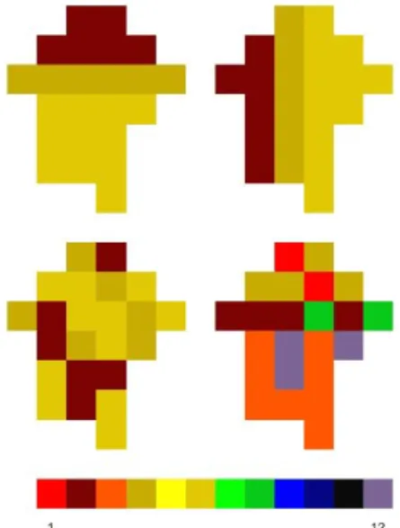
Figure 1 is a graphical representation that further clarifies exactly what this paper attempts to accomplish. In Fig. 1, the FFCO2 emissions from a hypothetical country are mapped. The total mass of emissions is identical in the four panels (in this paper, the uncertainty on the country total is not being examined), only the distribution methodology has changed. These different methodologies might represent different spa-tial proxies (e.g., the CDIAC population proxy), a bottom-up inventory approach (e.g., the VULCAN approach), or a hybrid approach (e.g., point sources and spatial proxies, e.g., ODIAC). Deciding which mapped distribution is best is made difficult by the lack of physical samples of FFCO2 at the spatial and temporal scales of interest. While two such maps can be superimposed and subjected to spatial analy-ses such as differencing, one gains little insight into an over-all superior mapping methodology. This paper aims to sup-plement the CDIAC maps with similar spatial and tempo-ral scale maps that represent the uncertainty in each map grid cell location. This should facilitate the determination of whether different emission maps are statistically differ-ent. More importantly, this should aid those who use these FFCO2 mass maps to better understand, model, and display the data by explicitly showing the uncertainty inherent in the maps.
Figure 1.Hypothetical FFCO2 mass maps for a hypothetical coun-try. The total mass of emissions is identical in the four panels; only the spatial distribution has changed between the panels. This paper aims to aid in the evaluation of such maps by supplying gridded un-certainty information at the same spatial and temporal scales as the emission maps. The scale is in arbitrary units.
2 A brief review of the CDIAC mapping process
The procedure for creating the CDIAC maps of FFCO2 emis-sions has remained remarkably stable since first published by Andres et al. (1996). The most notable changes since that publication have been the update and revision of data under-lying the CDIAC FFCO2 emissions time series and the mod-ification of the baseline geography map to account for the creation of new political units (e.g., the unification of Ger-many in 1990 or the breakup of the Soviet Union in 1991). Figure 2 shows the basic FFCO2 mass emissions map cre-ation process. The tabular FFCO2 emission data, by ncre-ation, are mapped to regions of the world using a 1◦ latitude by 1◦ longitude (1◦×1◦) map of geography (attributing grid
cells to a single country). The population distribution within a country, also at 1◦×1◦scale, is used as a proxy to
emis-FFCO2 DATA (TABULAR DATA)
Gridded FFCO (1
Figure 2.Basic CDIAC map creation process. The tabular FFCO2 emission data are mapped to regions of the world by the 1◦latitude by 1◦ longitude (1◦×1◦) map of geography with within-country FFCO2 distribution provided by the 1◦×1◦population distribution.
sions. The change in population proxies introduced in this paper is a departure from this former practice as now changes in magnitude shown in subsequent maps for a particular grid cell are due to a convolution of national FFCO2 emission changes and population density changes.
3 The new population proxy
Prior to this publication, CDIAC used a temporally fixed population proxy to distribute FFCO2 emissions within each country for all years (Andres et al., 1996). While working through the issues associated with this paper, it became clear that methodological improvements to the mapping process would improve the quality of both the magnitude maps and the uncertainty maps. The fixed population map originally reported in Andres et al. (1996) is still utilized for the years 1751–1989 since no better alternative has been identified for these years. Annually varying Global Population of the World (GPWv3, CIESIN and CIAT, 2005) maps are now used for the years 1990–1997. Annually varying LandScan (Dobson et al., 2000) maps are now used for years 1998– 2013 and are intended to be used for future years. The two new population data sets are not identical. GPWv3 estimates nighttime population (where people are at night) while Land-Scan estimates daytime population (where people are dur-ing the day). This change in population data sets does induce some variability in the results, but most populated grid cells are less than 10 % different between daytime and nighttime relative populations.
GPWv3 has three base years: 1990, 1995, and 2000. The original 2.5 min data (approximately 5 km at the equator) were aggregated to the 1◦ spatial resolution of the CDIAC 1◦×1◦maps. Data for 1991–1994 and 1996–1999 were
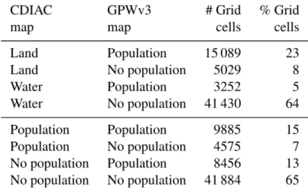
in-terpolated from the base years. Table 1 compares the annu-ally varying GPWv3 population maps to the CDIAC 1◦×1◦
geography and fixed population maps. Of the populated cells on the GPWv3 map, 5 % fall into cells labeled as water on
Table 1.Comparison of the year 1997 GPWv3 population map with CDIAC geography and fixed population maps. The number of wa-ter cells is less than 70 % of the total because 4550 ocean cells sur-rounding Antarctica are labeled as the Antarctic Fisheries, a United-Nations-named unit used to track energy consumption of Southern Ocean fishing fleets. CDIAC considers these Antarctic Fisheries cells as pseudo land cells (i.e., subject to emitting FFCO2). The year 2010 LandScan population map has a similar comparison to the CDIAC geography map (within 3 % in all categories) and pop-ulation map (within 4 % in all categories). CDIAC, GPWv3, and LandScan population maps all have land cells that are not popu-lated.
CDIAC GPWv3 # Grid % Grid
map map cells cells
Land Population 15 089 23 Land No population 5029 8
Water Population 3252 5
Water No population 41 430 64
Population Population 9885 15 Population No population 4575 7 No population Population 8456 13 No population No population 41 884 65
the CDIAC map; this 5 % of cells contains less than 5 % of the GPWv3 global population and are excluded from further analysis. Of the populated cells on the GPWv3 map, 13 % fall into unpopulated cells on the CDIAC map; these 13 % of cells contain less than 6 % of the GPWv3 global population. LandScan has maps for the years 1998 to 2012, except for 1999. As with the GPWv3 data, the original 30 s (a dis-tance unit, approximately 1 km at the equator) data were ag-gregated to the 1◦spatial resolution of the CDIAC 1◦×1◦
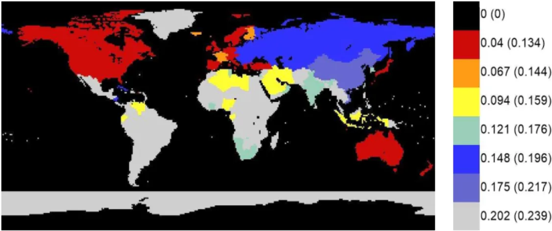
Figure 3.Tabular FFCO2 uncertainty assessment example. The plot is for the year 2010 and its key shows the annual uncertainty as a fraction. In parentheses, the monthly uncertainty is shown as a fraction. The two quantities shown have the same spatial extent; they differ only in magnitude. Different years would show slightly different spatial patterns as countries emerge or disappear from the FFCO2 tabular data.
The main effect of the new annually varying population maps used for the years 1990 to present is the appearance of FFCO2 emissions in grid cells that previously showed zero population and thus zero emissions. This spread in FFCO2 emissions for a given country is accompanied by a lower-ing of the average FFCO2 emission per grid cell (i.e., the same FFCO2 emission distributed amongst more grid cells). The new population maps also lead to some speckling in some map areas that previously appeared more homogeneous in FFCO2 emission magnitude. Finally, the new population maps increase the range of FFCO2 emissions displayed at both the lower and higher ends of emissions. Overall, the maps line up well with each other in geographic extent be-cause the same underlying 1◦×1◦geography map is used,
regardless of the population map used.
4 Uncertainty calculations
All three of the basic input data (i.e., tabular FFCO2 data, ge-ography map, and population map) contribute uncertainty to the final gridded FFCO2 mass emissions 1◦×1◦map. Each
of these inputs will be examined in turn, both in terms of the specific uncertainty they contribute as a data input, as well as the general uncertainty they contribute in their functional role of creating a final gridded FFCO2 mass map.
4.1 FFCO2 tabular data
The underlying FFCO2 tabular data contribute uncertainty to the final gridded FFCO2 mass map. In the case of the CDIAC FFCO2 mass maps, these data are the tabular FFCO2 esti-mates CDIAC reports for each country of the world, but the discussion here can be applied to all national FFCO2 emis-sions estimates.
The basic methodology to create the tabular CDIAC FFCO2 data is given in Marland and Rotty (1984). An-dres et al. (2012) expand upon this methodology and com-pare it to three other global FFCO2 tabular data sets. An-dres et al. (2014) describe a systematic uncertainty assess-ment of the CDIAC FFCO2 tabular data. No such similar un-certainty assessment has been published for the three other global FFCO2 tabular data sets. The uncertainty in the tabu-lar FFCO2 data is important as it provides the quantity that is eventually mapped. If the tabular FFCO2 data are uncertain, then the FFCO2 emissions distribution is uncertain.
Figure 3 displays the uncertainty assigned to different countries as described in Andres et al. (2014). The assign-ment was based upon grouping countries into seven differ-ent qualitative classes (Andres et al., 1996) based on similar energy and statistical infrastructures, which were later quan-tified in Andres et al. (2014). The quantification consisted of determining uncertainties for two of the classes and then doing a linear fit through the rest of the classes. Andres et al. (2014) describe the strengths and weaknesses of this ap-proach. As in Andres et al. (2014), the national FFCO2 un-certainty estimates used in this analysis remain fixed with time. Future versions of this work could utilize changing na-tional FFCO2 uncertainty estimates, but the existence of sup-porting data to rigorously support changing uncertainty esti-mates are lacking at this time.
para-graph. The monthly uncertainty is constant and at 2σ equals 12.8 % (Andres et al., 2011).
Both the tabular FFCO2 data and the national uncertain-ties used in this analysis are for apparent consumption data. Apparent consumption allows for the estimate of national FFCO2 emissions through the accounting of production, im-ports, exim-ports, etc., and thus allows the association of these FFCO2 emissions to geography. Andres et al. (2012) discuss the strengths and weaknesses of apparent consumption ver-sus production data. Production data are unsuitable for use in this analysis because their spatial domain is global (in terms of fuel consumption) and the focus here is on the uncertainty of 1◦×1◦mapped FFCO2 emissions.
Figure 3 shows an example of the national FFCO2 uncer-tainty assessment results. There are 64 unceruncer-tainty assess-ments completed for the annual 1950–2013 time series, each map reflecting the mix of countries that existed in a partic-ular year. Another 64 uncertainty assessments occur for the monthly 1950–2013 time series. The next section discusses the role geography plays in more detail.
4.2 Geography map
The underlying geography map contributes uncertainty to the final gridded FFCO2 mass map. In the case of the CDIAC FFCO2 mass maps, this geography map is a 1◦×1◦ raster
map, but the discussion here can be applied to all FFCO2 distribution mechanisms.
The CDIAC geography map is a 1◦×1◦ raster of world
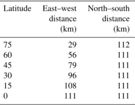
political units. Raster implies that the world is depicted in a regular grid pattern with the underlying geography rep-resented by a single value in the grid (Fig. 4). This distin-guishes it from other possible spatial representations such as mixed raster where the grid cell may contain more than one geography value and vector where polygons instead of grids are used to represent an area. A raster map was chosen for the CDIAC FFCO2 mass maps because of its relative simplic-ity, full global coverage, and ease with which its results can be implemented into models (e.g., carbon cycle models). A drawback of the raster map is its distortion of the surface area of the Earth (Table 2), which appears as square grid cells in the traditional CDIAC representation of its FFCO2 gridded data.
While Fig. 4 is simple in concept, it is illustrative of uncertainty inherent in raster maps of geography. Many of these sources of uncertainty arise because of map scale. For example, the Northwest Angle is territory of the contigu-ous US that lies entirely north of 49◦ latitude, the
north-ern border observed for the westnorth-ern portion of the con-tiguous US. This part of the state of Minnesota is more than 1500 km2 in area, has a population greater than 100, and has roads, an airport, a school, businesses, and cus-toms and immigration control. However, on the CDIAC 1◦×1◦ geography map, this area appears as Canada
be-cause of its small area relative to the more dominant area
Figure 4.Raster representation. The left figure shows two hypo-thetical regions labeled A (purple) and B (yellow). The right figure shows the raster version of this geography where the dominant spa-tial region in each grid cell on the left becomes the value of the grid cell on the right. Other potential representations include mixed raster and vector (see text for description).
Table 2.Selected latitudes and the length dimensions of 1◦in as-sociated raster cells. The values shown are symmetric about the equator. CDIAC locates its raster borders on 1◦lines of latitude and longitude. Other maps may center their raster cells on these lines and are thus offset from the CDIAC grid by 0.5◦. Calcula-tions based on WGS84 ellipsoid data from http://earth-info.nga.mil/ GandG/coordsys/csatfaq/math.html.
Latitude East–west North–south distance distance
(km) (km)
75 29 112
60 56 111
45 79 111
30 96 111
15 108 111
0 111 111
of Canada in its grid cell. Another uncertainty example in-volves surveying errors. While Colorado in the US was orig-inally defined along lines of latitude and longitude, sur-vey errors resulted in several kinks along its borders, which have been codified into law (http://mathtourist.blogspot.com/ 2007/08/rectangular-states-and-kinky-borders.html). On the Colorado–New Mexico border, this kink is approximately 2 km – too small to be seen in the CDIAC 1◦×1◦
geogra-phy map, but of concern for finer scale maps.
C C D
Fi er scale Coarser scale
k k
Figure 5.Spatial rescaling issues. The blue area represents ocean and the green area represents land. A hypothetical rescaling from 1 to 5 km is shown. Note that cell C in the finer scale resolution has been recoded to ocean in the coarser resolution. In rescaling FFCO2 mass maps, this recoding is often accompanied by the movement of FFCO2 from cell C to cell D.
Dependent on location, these disputes have varying impact on the FFCO2 emissions distributions.
A final geography uncertainty arises from spatial rescaling as shown in Fig. 5. Here, a finer spatial scale map is rescaled to a coarser grid. A common outcome of this procedure is to name the left coarser grid cell ocean, name the right coarser grid cell land, and move the carbon that was in that left grid cell to the right grid cell. This movement accommodates not having FFCO2 being emitted from an ocean grid cell and maintaining full FFCO2 accounting.
Geography contributes uncertainty to the final FFCO2 mass map. Since the identity of an interior grid cell of a large homogeneous political unit is unambiguous (e.g., the geo-graphic center of a country greater than or equal to 3 by 3 grid cells in size), the uncertainty is concentrated around the borders and may be due to map scale issues, political issues, or rescaling, as the examples above illustrated. As the exact map scale changes, the nature of the uncertainty may change, but it does not disappear. The uncertainty in the geography map is important because the map is used to locate the tabu-lar FFCO2 data. If the geography map is uncertain, then the FFCO2 emissions distribution is uncertain.
To assess uncertainty due to the geography map, the al-gorithm shown in Fig. 6 was used. The central grid cell A is assessed for uncertainty based upon the values of the sur-rounding eight grid cells. The simplest case is if all surround-ing eight cells are of the same value as the central cell. In this case, geography lends 0 % uncertainty to the identity of the central cell. This is the most common case (63.6 %) in the CDIAC geography 1◦×1◦maps.
This simple approach does exclude enclaves, territories that are completely surrounded by other territories, which could be problematic in some locations. For example, the Spanish town of Llívia, for political and historical reasons, is completely surrounded by French territory. On the CDIAC 1◦×1◦ map, this specific example is ignored due to map
scale, but on a 1 km scale map it should not be ignored. For the CDIAC geography 1◦×1◦ map, enclaves
(includ-ing small island nations) and other small-area political units
A
Similar cells Uncertainty % of total 0/8 100% 0.4 1/8 87.5% 0.6 2/8 75% 1.4 3/8 62.5% 3.1 4/8 50% 6.0 5/8 37.5% 11.4 6/8 25% 6.3 7/8 12.5% 7.2
8/8 0% 63.6
Figure 6.Geography map uncertainty is assessed by a 3×3 mov-ing window. The central grid cell A is assessed for uncertainty based upon the values of the surrounding eight grid cells. If no surround-ing cells equal the value of the central cell, then the uncertainty on the central cell is 100 %. After assessment of one cell, the 3×3 window moves to assess the next cell until all cells are assessed. The accompanying table gives cell matches, resulting uncertainties, and percentage of land cells that fit each uncertainty.
were not ignored if their occurrence only appeared in one grid cell on the entire global map. Then, the spatial domi-nance of the grid cell was ignored so that the small-area po-litical unit would be represented and its associated tabular FFCO2 not lost from the final mapped product.
On the other end of the spectrum, if no surrounding cells equal the value of the central cell (e.g., a small island nation), then the uncertainty on the central cell is 100 %. An example of this situation can be seen in Fig. 4 where there is ambigu-ity in all of the eight surrounding cells as to whether the cen-tral cell value encroaches on the territory of the surrounding cells. A worst case scenario for the CDIAC 1◦×1◦FFCO2
mass maps, leading to a 100 % uncertainty contribution by the geography map, is shown in Fig. 4 if the island is com-pletely uninhabited except for a capital city existing in one of the surrounding cells. In this case the island population would be moved to the central cell, the only cell containing area for this country. Thus, the result would be FFCO2 emis-sions located in a cell one grid cell removed from its true lo-cation. This is the least common case (0.4 %) in the CDIAC geography 1◦×1◦maps.
Intermediate between these two end member cases dis-cussed are all other border configurations. The accompany-ing table in Fig. 6 gives cell matches and resultaccompany-ing uncertain-ties. After assessment of one cell, the 3×3 window moves
Figure 7.Geography map uncertainty assessment examples. The top plot is for the year 1950 and its key shows the uncertainty as a fraction. The bottom plot shows the 1950–2011 differences. A difference plot was shown because only 749 cells (about 1 % of 64 800 total cells) changed value between 1950 and 2011.
Figure 7 shows an example of the geography map uncer-tainty assessment results. There are 64 unceruncer-tainty assess-ments completed for the 1950–2013 time series, each map re-flecting the mix of countries that existed in a particular year. The difference plot is shown in Fig. 7 to highlight some of the changes over time, most notably in Africa, Europe, and Asia. There are no differences between geography map uncertainty for annual and monthly FFCO2 time series.
Geography map uncertainty can expand internally within nations as individual states or provinces have local FFCO2 emissions mapped. This has not been implemented to date in CDIAC 1◦×1◦ maps, but other mapped FFCO2 emissions
distributions may need to incorporate such effects. The next section discusses in more detail the role the population proxy plays.
4.3 Population map
The underlying distribution proxy contributes uncertainty to the final gridded FFCO2 mass map. In the case of the CDIAC FFCO2 mass maps, this proxy is a population distribution map, but the discussion here can be applied to all distribution mechanisms.
CDIAC distributes FFCO2 emissions within a country in direct proportion to the population distribution. In effect, the
CDIAC methodology assumes that each country has fixed per capita FFCO2 emissions across all its territory. While not the best assumption, it was considered the best avail-able option at the time the CDIAC 1◦×1◦maps were first
created in 1993. Today, producers of other FFCO2 emissions distributions have taken advantage of newer data sets, includ-ing updated population distributions, power plant locations, road and rail networks, traffic counts, etc., to act as proxies for FFCO2 emissions distribution (e.g., Olivier et al., 2005; Gurney et al., 2009; Rayner et al., 2010; Oda and Maksyutov, 2011; Wang et al., 2013).
The uncertainty in the population map is important be-cause the map is used to perform the within-country FFCO2 emissions distribution. If the population map is uncertain, then the FFCO2 emissions distribution is uncertain. Two issues are of concern here. First, how accurately does the population proxy mirror FFCO2 emissions? Second, since CDIAC uses a fixed population proxy for some years, how has the within-country population distribution changed with time? Both of these issues will be examined in turn.
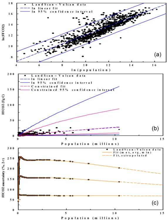
be-Figure 8.The population–FFCO2 emissions relationship. Upper panel: independent data sets of population and FFCO2 emissions are ag-gregated to 1◦resolution and spatially matched. Dropped from the figure are three data points that had positive FFCO2 emissions and zero population and 67 data points where positive FFCO2 occurred in cells subject to population from an adjacent country. These cells may in-clude adjacent country population but not the FFCO2 emissions attributable to that population, thus degrading the desired population–FFCO2 emissions relationship. In addition to the 849 data points, a linear fit and 95 % confidence interval are shown. Middle panel: same data as seen above except on linear axes. Monte Carlo analyses provided a constrained linear fit and 95 % confidence interval with the constraint that the total mass of the system is constant and using a robust estimate of the data distribution. Lower panel: population–FFCO2 emissions 2σ relationships extracted from the Monte Carlo analyses. Extraction is dashed where extrapolated.
cause, by definition, a linear regression between population and FFCO2 emissions results in an r2value of one, perfect correlation for data from one country. While this same re-gression could be applied to the global CDIAC data,
Since the CDIAC data are unsuitable to test the popula-tion proxy uncertainty, and since there are insufficient ac-tual measurements of FFCO2 emission rates at the appropri-ate spatial and temporal scales, independent population and FFCO2 emission distributions will be used to assess the pop-ulation proxy uncertainty. The poppop-ulation distribution used is the global 30 min (spatial scale) LandScan data product; it was produced without consideration of FFCO2 emissions. The FFCO2 distribution used is the 1/10◦Vulcan data prod-uct for the contiguous 48 US states (Gurney et al., 2009); it was produced with minimal use of population data (via cen-sus data and not LandScan data, although LandScan has roots to census data). The Vulcan data product is the most expan-sive (in terms of spatial coverage) that relies least heavily on population for its FFCO2 emission distribution. Figure 8 shows the results of this assessment.
The upper panel of Fig. 8 shows the relationship between the independent data sets of LandScan population and Vulcan FFCO2 emissions for the contiguous US for the year 2002, the baseline map of the Vulcan emissions. The data axes have been transformed into natural log scales to allow for easy extraction of basic statistical parameters (i.e., the linear fit and 95 % confidence interval). The middle panel shows these same data and statistical parameters on linear scales. The spread of data around the linear fit shows the nonlinearity, and thus the nonuniform per capita relationship, of the data. The initial 2σ confidence interval on the linear scale is not ideal for constraining uncertainty on the population–FFCO2 emissions relationship.
To reduce the initial 2σ confidence interval on the linear scale (and thus the effect of data outliers), a Monte Carlo analysis (MC) was performed. Input into the MC included two pieces of information. First, a reduced version of the original input data set was created by excluding data points that existed outside of±2σ, reducing the 849 point data set to 793 data points. A linear fit and standard deviation were calculated from the 793 points. Second, the total carbon of the system is constant. The MC proceeded then by selecting one of the original 849 populations, calculating the reduced version regression fit FFCO2 emission for that population, and adjusting that FFCO2 emission by the reduced version standard deviation multiplied by a randomly selected stan-dard deviation interval from a normal curve. After repeating the MC process for all 849 populations, if the sum of bon from all 849 populations was not equal to the input car-bon, the MC run was discarded. If the sum was equal, the MC results were kept and the MC process was repeated un-til 1000 successful runs (i.e., constant carbon achieved) were completed. From the 1000 MC runs, then an average FFCO2 emission and 2σinterval were calculated at each population. Testing revealed that 1000 MC runs was sufficient for the av-erage and 2σ interval to stabilize.
The lower panel of Fig. 8 shows this population–FFCO2 emissions 2σ relationship in percentage units. Since the 2σ
intervals in the upper and middle panels are not symmetrical
about the best fit lines, the lower panel shows the maximum and minimum value of the 2σ interval. Values for the maxi-mum 2σ distance were derived from the−2σ curve at low population values and from the+2σcurve at high population values. Values for the minimum 2σ distance were derived from the+2σ curve at low population values and from the
−2σ curve at high population values. The relationships are dashed for populations not included in the LandScan popula-tion input data set.
The lower panel of Fig. 8 also shows the average 2σ
distance. Lacking further guidance as to the nature of the population–FFCO2 emissions relationship, the average is used to describe the relationship. Note that the use of the maximum or minimum curves would result in different un-certainties to be calculated and these may be more appro-priate than the average. Future study and data may guide a more appropriate choice. The results from the lower panel of Fig. 8 are also extrapolated from the contiguous US to the en-tire world for the uncertainty analysis. Future study and data may also provide a more robust relationship.
It is not expected that the exact population–FFCO2 emis-sions relationship shown in the lower panel of Fig. 8 will hold at 0.25, 0.1, and 0.01◦ spatial resolution, resolutions being utilized by other groups today. Likewise, it is not expected that the exact population–FFCO2 emissions rela-tionship shown in the lower panel of Fig. 8 will be useful for other maps that use proxies in addition to population to distribute FFCO2 emissions because these other proxies will change the population–FFCO2 relationship. The results shown in Fig. 8 are specific to 1◦resolution using population
as the sole distribution proxy.
The large uncertainty bounds on the carbon–population re-lationship are hypothesized to be due to large point sources incorporated in some 1◦×1◦ grid cells and not others. In
these cells, FFCO2 emissions are decoupled from popu-lation. Support for this comes from Singer et al. (2014), who showed a relatively flat per capita FFCO2 relation-ship, as compared to the relationship derived here. Singer et al. (2014) derived this flat per capita by taking state level emissions, subtracting emissions from large point sources in each state, and then calculating per capita emissions. The ro-bust 2σ interval used in the constrained fit of Fig. 8 poten-tially removes some, but not all, of these large point source 1◦×1◦grid cells. While the process used here could be
iter-ated to achieve results similar to Singer et al. (2014), that has not been pursued at the present time since that effort would not be representative of the CDIAC FFCO2 mapping pro-cess.
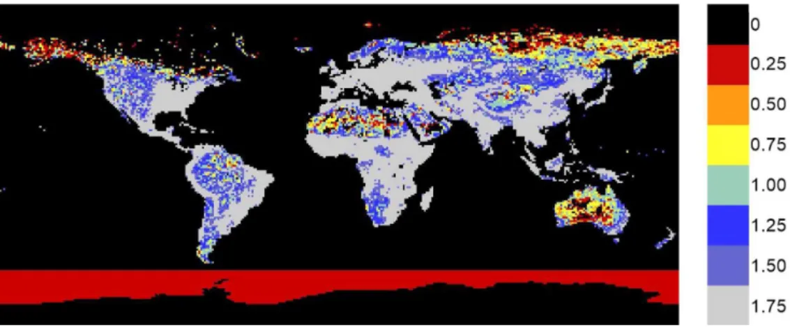
Figure 9.Population map uncertainty assessment example. The plot is for the year 2011 and its key shows the annual uncertainty as a fraction where 1.75 is 175 % uncertainty. This map was generated by the average relationship seen in the lower panel of Fig. 8.
one proxy to distribute FFCO2 emissions is to take FFCO2 from one cell and place it in another cell. The result of this redistribution procedure can increase or decrease the slope of the population–FFCO2 emissions relationship as well as increase or decrease the 2σ distance at a given population. The addition of more than one distribution proxy is what Singer et al. (2014) utilized, which resulted in a relatively flat per capita FFCO2 relationship for non-point source FFCO2 emissions.
Figure 9 shows an example of the population map uncer-tainty assessment results. There are 64 unceruncer-tainty assess-ments completed for the 1950–2013 time series, with each map reflecting the population that existed in a particular year for the given set of countries. These maps were generated by the average relationship seen in the lower panel of Fig. 8. For countries that only occupy one grid cell, their uncertainty was set to zero since the relationship derived in Fig. 8 is not applicable. There are no differences between population map uncertainties for annual and monthly FFCO2 time series.
Figure 9 shows that the majority of the land mass is cov-ered in uncertainties greater than 100 %. This could be used as evidence to argue against using population as a distribu-tion proxy, assuming a better alternative can be found.
To address the second concern, population changes with time, it is assumed that the annually varying population maps used for the years 1990 to present capture relative changes and are thus not a concern. However, the pre-1990 years use a fixed population map and this may be of concern. An-nual maps of GPWv3 and LandScan were used to assess the changes in relative population density within each country on an annual basis. The final result of this assessment was that population changes with time induce little uncertainty into the overall FFCO2 distribution globally when a fixed popu-lation proxy is utilized. In specific 1◦×1◦cells, the change
can appear dramatic when a cell goes from having zero popu-lation to being populated. However, the vast majority of pop-ulated cells do not show this change in any given year. The
average populated 1◦×1◦cell shows less than a 0.1 % uncer-tainty introduced over 10 years, which is far smaller than the other uncertainties examined in the paper. Thus, uncertain-ties introduced by population changes with time are not con-sidered further in this paper. The next section combines the uncertainty maps from the three components just discussed.
4.4 FFCO2 map uncertainty
Figure 10 shows the uncertainty by combining two compo-nents: FFCO2 tabular data and geography. This intermedi-ary step is shown because it demonstrates the order of un-certainty (ranging from < 10 to 102 %) that will be associ-ated with all gridded FFCO2 data products that have roots similar to the CDIAC data product. This particular presenta-tion ignores the within-country distribupresenta-tion proxy, only bor-ders and national FFCO2 magnitude are included. The two-component uncertainty shown is the square root of the sum of the squares of the individual components (i.e., Figs. 3 and 7) as each component is independent of the other. Figure 10 does not show many changes temporally (only 809 of 64 800 cells change values from the years 1950 to 2011), but there is much spatial variability within a given year.
Figure 10. Two-component 2σ uncertainty derived from FFCO2 tabular data and geography.
in the year 1950 due to the inclusion of the annually varying population proxy.
Thus, this gridded product (i.e., Fig. 11) incorporates all known and deemed-significant uncertainty from the spatial resolution, temporal resolution, and underlying FFCO2 es-timation process. For the years 1950–2013, 64 such maps exist. It is expected that future releases of the annual and monthly CDIAC 1◦×1◦FFCO2 mass maps will be
accom-panied by similarly spatially and temporally scaled 1◦×1◦
uncertainty maps.
The 193 % maximum 2σ uncertainty occurs regardless of whether the old fixed population proxy or the new annually varying population proxy is used. This is because the peak in the carbon–population relationship occurs at relatively low population values, around 172 000 people per 1◦ grid cell
(Fig. 8, lower panel). This is far removed from the maximum populated grid cells, which the annually varying population proxy better captures.
For the 2011 1◦×1◦uncertainty map, of the 25 095 cells
that have a non-zero uncertainty associated with them, 22 % of these are dominated by uncertainty contributed by the FFCO2 tabular data (Fig. 3), 27 % of these are dominated by uncertainty contributed by geography (Fig. 7), and 51 % are dominated by uncertainty contributed by population (Fig. 9). Tabular FFCO2 data dominate uncertainty in areas of low to no population. Geography dominates uncertainty around borders shared with water bodies. Population dominates un-certainty in the rest of the populated world.
Figure 11.Three-component 2σuncertainty.
4.5 Other sources of uncertainty
Not explicitly considered here are autocorrelations of uncer-tainty in the combined spatiotemporal domain. For example, if the local power plant is shut down for maintenance, other power plants located on the same electrical grid may increase electricity production, and hence FFCO2 emissions, to main-tain overall grid power levels for an electricity demand that is independent of the local power plant maintenance sched-ule. In actual cases of this scenario, of which the authors are aware, the relatively coarse CDIAC 1◦×1◦annual scale map
was partially insensitive to this maintenance. That is because some of the power plants that increased electricity production were located in the same 1◦×1◦cell as the local power plant,
and thus the FFCO2 emissions were still accurately captured in that cell. The uncertainty assessment presented here is un-affected by this maintenance and redistribution of power gen-eration. However, some of the power plants that increased electricity production were located outside the local power plant 1◦×1◦cell. The uncertainty assessment presented here
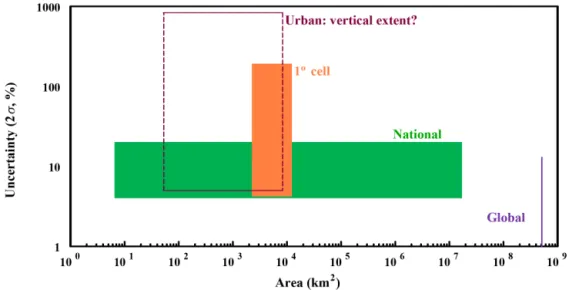
Figure 12.CDIAC experience regarding resolution and uncertainty. Here, the focus is on spatial resolution, but CDIAC also noticed a similar relationship in temporal scales going from annual to monthly to daily to hourly. The uncertainty on urban scale maps is largely unknown at present.
5 Discussion
Uncertainty generated by using the population map dom-inates the gridded FFCO2 uncertainty. Population is one proxy used to distribute FFCO2 emissions that has detail in both time and space. Many of the proxies used by other map distribution algorithms lack this detail in time and space. Population was also the only useful global proxy available in 1996 when the CDIAC 1◦×1◦ maps were first published.
Many of the proxies used by other map distribution algo-rithms came into being after 1996. Finally, national popu-lations directly use energy and emit FFCO2 in many sectors of the economy. Other map distribution algorithms attempt to improve this relationship by parsing portions of FFCO2 emissions not directly related to national populations (e.g., electricity power plant emissions) and using other proxies to distribute these non-population-related FFCO2 emissions.
The linear fit that CDIAC employs for FFCO2 emissions distribution (i.e., the population map) comes with the cost of introducing uncertainty due to the lack of a one-to-one re-lationship. However, this is true with other proxies because they also lack the one-to-one relationship. It is important to remember why these proxies are utilized: a lack of actual measurements of FFCO2 emission rates at the appropriate spatial and temporal scales. Here, a compromise is intro-duced into the mapping process: distribution proxies with their associated uncertainties are balanced against computa-tion and data gathering costs. In general, for full global cov-erage, finer spatial and temporal resolution proxies introduce more uncertainty than coarser spatial and temporal resolu-tion proxies. This higher uncertainty is often rooted in less certain data in all grid cells due to the lack of resources to appropriately monitor all grid cells at the desired spatial and
temporal resolutions. This intermingling of spatial and tem-poral resolution is key. Most high-spatial-resolution proxies are sampled for only short temporal durations or limited spa-tial extents. Most high-temporal-resolution proxies are sam-pled for limited spatial extents or limited temporal durations. Figure 12 is a summary of the CDIAC experience regarding resolution and uncertainty. As spatial scales decrease, uncer-tainty increases. Much effort is now being directed into pro-ducing urban scale maps, but their uncertainty at present is largely unknown.
Table 3.Comparison of INFLUX airplane-based results, Hestia, and the CDIAC 1◦×1◦map. All values reported in Tg C. Reported in parentheses are 1σ and 2σ mass ranges. Cambaliza et al. (2014) report airplane-based results for 1 March, 29 April, and 1 June 2011 of 11 000, 7500, and 26 000 mol s−1, respectively. Unit conversion equate these values to 4.2, 2.8, and 9.8 Tg C yr−1. The 5.6 Tg C average is reported above. For monthly samples, a similar unit conversion was completed. For both annual and monthly cases, the Cambaliza et al. and Hestia results were scaled up to the temporal resolution of the CDIAC data.
CDIAC Cambaliza et al. (2014) Hestia
Annual 7.7 (1.7–14, 0–20) 5.6 (2.8–8.4, 0.0–11) 4.4 (4.1–4.9, 3.8–5.3) March 0.68 (0.1–1.2, 0–1.7) 0.35 (0.18–0.53, 0.0–0.71) 0.39 (0.36–0.43, 0.33–0.47) April 0.61 (0.1–1.1, 0–1.6) 0.23 (0.12–0.35, 0.0–0.47) 0.33 (0.31–0.37, 0.28–0.40) June 0.62 (0.1–1.1, 0–1.6) 0.81 (0.40–1.2, 0.0–1.6) 0.38 (0.35–0.42, 0.32–0.45)
Table 4.This work versus alternative formulation of the gridded map uncertainty at annual timescales. Minimum, average, maxi-mum, and standard deviation (SD) of three-component 2σ uncer-tainty for populated and FFCO2-emitting grid spaces. All values in percent. See text for parameters of the alternative formulation.
Minimum Average Maximum SD
This work 4.0 120 190 51
Alternative 4.0 65 94 22
formulation
While there is lack of actual measurements of FFCO2 emission rates at the appropriate spatial and temporal scales of the CDIAC 1◦×1◦maps, a sampling effort that partially
approaches these scales occurred in Indianapolis, US, dur-ing the Indianapolis Flux Experiment (INFLUX). Cambal-iza et al. (2014) report on airplane-obtained CO2flux mea-surements for three dates in 2011. Their meamea-surements show “considerable day-to-day variability” and include all CO2 fluxes, not just FFCO2. However, with reason, they assume their results are mostly sensitive to FFCO2. Table 3 compares their results to the CDIAC 1◦×1◦ map grid cell that
con-tains Indianapolis. While there are still mismatches in tem-poral and spatial scales (and potentially CO2 sources), the results are within the 1σ uncertainty bounds of each other at annual timescales. At monthly timescales, the comparison is not so favorable: all of the Cambaliza et al. (2014) results fall within the CDIAC 1σ uncertainty; only one CDIAC month falls within the Cambaliza et al. (2014) 1σ uncertainty, one CDIAC month falls within the Cambaliza et al. (2014) 2σ
uncertainty, and the other month falls outside the Cambaliza et al. (2014) 2σ uncertainty.
INFLUX was also aided by a bottom-up inventory, Hes-tia (Gurney et al., 2012), which is a detailed building-by-building, street-by-street, hourly FFCO2 emissions inven-tory, downscaled from VULCAN. Cambaliza et al. (2014) report Hestia inventory values for the same dates (Table 3). While there are still mismatches in temporal and spatial scales at both annual and monthly timescales, the Hestia re-sults fall within the CDIAC 1σ uncertainty and the CDIAC
results do not fall within the Hestia 2σuncertainty. Similarly, the Cambaliza et al. (2014) data and Hestia results also do not always fall within each others’ 1 or 2σ uncertainty bounds.
Singer et al. (2014) show that for the contiguous US, when large point sources are removed from the CDIAC 1◦×1◦
maps and separately placed with their emissions, the remain-ing FFCO2 emissions show relative constancy on a per capita basis. If this result can be verified elsewhere and if a robust large point source database can be developed at appropriate spatial and temporal scales, this may lead to better global maps of FFCO2 emissions. While current large point source databases have known spatial deficiencies (e.g., Oda and Maksyutov, 2011; Nassar et al., 2013; Woodard et al., 2015), these spatial deficiencies can be overcome with additional geolocation efforts. Current large point source databases are usually based on a certain point in time and offer little to no temporal information. This temporal information is cru-cial for appropriately assigning magnitudes to FFCO2 emis-sions from these locations. Magnitude variations can occur on all temporal scales from minutes to years as energy de-mand changes, new units are installed, and old units are unin-stalled or shut down for maintenance. The uncertainty associ-ated with these temporal variations is unquantified at present. A commonly observed human tendency is to underesti-mate the uncertainties in our work. Going into this grid-ded uncertainty assessment, when asked about the quality of the CDIAC 1◦×1◦ FFCO2 mass magnitude maps, the
uncer-tainty) of Hogue et al. (2016), but does allow for locations to be located to within one-half of a 1◦ grid cell. While there
are examples of 1◦uncertainty (e.g., see Sect. 4.2 geography
map), these examples are an isolated few and may represent the outliers beyond 2σ. For the population map, uncertainties are reduced to the minimum line of Fig. 8. FFCO2 emissions tabular data remain unchanged since no viable alternative assumption exists. The alternative formulation to the grid-ded map uncertainty results is roughly a halving of the aver-age, maximum and standard deviation values from the values originally reported in this work. The minimum value remains the same. The alternative formulation is simply the result of different assumptions and decisions being made during the uncertainty assessment process. At present, it is neither bet-ter nor worse than the uncertainties presented in Fig. 11. The alternative formulation is simply different from the main line of investigation that led to Fig. 11. What the alternative for-mulation really highlights is the need for additional work in this area and the need for physical sampling of FFCO2 emis-sions at appropriate spatial and temporal scales.
Table 4 also shows the average 2σ uncertainty value at 120 % for the work presented here. This is only slightly higher than the average 1σ uncertainty value of 50 % (2σ
100 %) presented by Rayner et al. (2010) for FFDAS at 0.25◦ resolution. These larger values are expected since the treat-ment here is more comprehensive than that of Rayner et al. (2010), incorporating non-zero uncertainty for the pop-ulation component, a more diverse and wider range of un-certainties for the FFCO2 tabular data, not clipping higher uncertainty values (200 % 1σ in the Rayner et al., 2010 as-sessment), and utilizing many more Monte Carlo simulations in realization of the FFCO2 distribution results (1000 vs. 25). The uncertainty bounds presented here (e.g., Fig. 11) are large. That may argue for a new approach to mapping FFCO2 emissions globally. The multi-proxy approach initially ap-pears promising because large fractions of FFCO2 emissions can be geolocated with much less spatial uncertainty than the population proxy provides. However, the databases com-monly used to provide the geolocation usually fail to pro-vide temporal information, making temporal uncertainty in-crease, sometimes substantially. Studies like INFLUX also initially appear promising with their high spatial and tem-poral resolutions often accompanied by lower uncertainties than those offered here (e.g., Fig. 11). However, INFLUX was a multi-million dollar campaign that gave good informa-tion on one grid cell out of 64 800 (temporally, different data streams lasted days to years). This approach is too expensive for global application with current resources. Satellites could offer high spatial and temporal resolution. However, current technology only senses field-of-view CO2, including the net effects of all sources and sinks on a parcel of air. Models are then needed to tease out the FFCO2 component.
Going forward, there may be multiple opportunities to improve FFCO2 mass maps by incorporating new data and proxies that were previously unavailable. Besides population,
few proxies currently in use have reliable histories longer than a few decades, and thus there may not be many ways to improve the historical record of emissions and their global distribution. Looking forward, existing and new technologies and techniques may provide continuous and detailed space and time data from which to better estimate and map FFCO2 emissions.
Hanging over all of these approaches to mapping FFCO2 emissions are planned, existing, and committed national and international agreements to limit future FFCO2 emissions. How these will be measured, reported, and verified (MRV) remains to be seen. This MRV task becomes only more daunting when uncertainties are used in the MRV process, in addition to the central best estimate of FFCO2 (and other) fluxes affecting the atmosphere (and climate) in which we live.
6 Conclusions
This paper provides (1) the first, gridded, comprehensive uncertainty estimates of global FFCO2 emissions, (2) a methodology that can be applied to other global FFCO2 mass maps, (3) a reminder to the community that FFCO2 has un-certainty both in tabular mass totals and in map-distributed masses, (4) a beginning for the broader community to sta-tistically compare different FFCO2 distribution maps (once uncertainty evaluations are completed on the other maps) to help determine better FFCO2 distribution algorithms, and (5) the basis for an improved understanding of the global car-bon cycle and its components by providing an uncertainty estimate for the CDIAC FFCO2 mass maps that can then be propagated into the rest of the global carbon cycle.
While more detailed proxies (in space, time, or num-ber) may lead to more visually appealing representations of FFCO2 emissions, that increased detail often brings in-creased uncertainty, thus obscuring the perceived increase in detail. The alternative formulation presented in Table 4 shows how easy it is to achieve lower reported uncertain-ties. While uncertainty is large at the per grid cell basis, Fig. 12 suggests that uncertainty decreases with aggregation to larger grid cells. While the exact map distribution mech-anism used here – per capita FFCO2 emissions by coun-try – largely determines the uncertainty associated with the CDIAC 1◦×1◦ maps, other map distribution mechanisms
likely follow a similar pattern: increasing uncertainty with decreasing spatial (and temporal) scale(s).
pi-oneering efforts in quantifying global and national FFCO2 emissions led to new carbon and climate understanding.
7 Data availability
The data for this paper are available at the CDIAC website (http://cdiac.esd.ornl.gov/trends/emis/meth_reg.html, An-dres and Boden, 2016a, b). FFCO2 emissions data are also currently available there (Boden et al., 2016). At the time of ACPD submission, the authors were in the process of updating the emissions data to the year 2013 (from 2011). That update is now complete and FFCO2 emission data and uncertainty maps up to the year 2013 are available from the CDIAC web site.
Acknowledgements. Ray Nassar and an anonymous reviewer
provided thoughtful comments and suggestions.
Edited by: Q. Zhang
Reviewed by: Nassar and one anonymous referee
References
Andres, R. J., Marland, G., Fung, I., and Matthews, E.: A one degree by one degree distribution of carbon dioxide emissions from fossil fuel consumption and cement manu-facture, 1950–1990, Global Biogeochem. Cy., 10, 419–429, doi:10.1029/96GB01523, 1996.
Andres, R. J., Fielding, D. J., Marland, G., Boden, T. A., Kumar, N., and Kearney, A. T.: Carbon dioxide emissions from fossil-fuel use, 1751–1950, Tellus, 51, 759–765, doi:10.1034/j.1600-0889.1999.t01-3-00002.x, 1999.
Andres, R. J., Marland, G., Boden, T., and Bischof, S.: Carbon diox-ide emissions from fossil fuel consumption and cement manu-facture, 1751–1991, and an estimate of their isotopic composi-tion and latitudinal distribucomposi-tion, in: The Carbon Cycle, edited by: Wigley, T. M. L. and Schimel, D. S., Cambridge University Press, Cambridge, 53–62, 2000.
Andres, R. J., Gregg, J. S., Losey, L., Marland, G., and Boden, T. A.: Monthly, global emissions of carbon dioxide from fos-sil fuel consumption, Tellus B, 63, 309–327, doi:10.1111/j.1600-0889.2011.00530.x, 2011.
Andres, R. J., Boden, T. A., Bréon, F.-M., Ciais, P., Davis, S., Erick-son, D., Gregg, J. S., JacobErick-son, A., Marland, G., Miller, J., Oda, T., Olivier, J. G. J., Raupach, M. R., Rayner, P., and Treanton, K.: A synthesis of carbon dioxide emissions from fossil fuel com-bustion, Biogeosciences, 9, 1845–1871, doi:10.5194/bg-9-1845-2012, 2012.
Andres, R. J., Boden, T. A., and Higdon, D.: A new eval-uation of the uncertainty associated with CDIAC estimates of fossil fuel carbon dioxide emission, Tellus B, 66, 23616, doi:10.3402/tellusb.v66.23616, 2014.
Andres, R. J. and Boden T. A.: Annual Fossil-Fuel CO2 Emissions: Uncertainty of Emissions Gridded by One De-gree Latitude by One DeDe-gree Longitude, Carbon Dioxide
Information Analysis Center, Oak Ridge National Labora-tory, US Department of Energy, Oak Ridge, Tenn., USA, doi:10.3334/CDIAC/ffe.AnnualUncertainty.2016, 2016a. Andres, R. J. and Boden T. A.: Monthly Fossil-Fuel CO2
Emissions: Uncertainty of Emissions Gridded by One De-gree Latitude by One DeDe-gree Longitude, Carbon Dioxide Information Analysis Center, Oak Ridge National Labora-tory, US Department of Energy, Oak Ridge, Tenn., USA, doi:10.3334/CDIAC/ffe.MonthyUncertainty.2016, 2016b. Boden, T. A., Marland, G., and Andres, R. J.: Global,
Re-gional, and National Fossil-Fuel CO2Emissions, Carbon Diox-ide Information Analysis Center, Oak Ridge National Labo-ratory, US Department of Energy, Oak Ridge, Tenn., USA, doi:10.3334/CDIAC/00001_V2015, 2015.
Boden, T. A., Andres R. J., and Marland, G.: Global, Re-gional, and National Fossil-Fuel CO2Emissions, Carbon Diox-ide Information Analysis Center, Oak Ridge National Labo-ratory, US Department of Energy, Oak Ridge, Tenn., USA, doi:10.3334/CDIAC/00001_V2016, 2016.
Cambaliza, M. O. L., Shepson, P. B., Caulton, D. R., Stirm, B., Samarov, D., Gurney, K. R., Turnbull, J., Davis, K. J., Possolo, A., Karion, A., Sweeney, C., Moser, B., Hendricks, A., Lauvaux, T., Mays, K., Whetstone, J., Huang, J., Razlivanov, I., Miles, N. L., and Richardson, S. J.: Assessment of uncertainties of an aircraft-based mass balance approach for quantifying urban greenhouse gas emissions, Atmos. Chem. Phys., 14, 9029–9050, doi:10.5194/acp-14-9029-2014, 2014.
CIESIN: Center for International Earth Science Information Net-work and Centro Internacional de Agricultura Tropical (CIAT).: Gridded Population of the World Version 3 (GPWv3): Popu-lation Grids, Palisades, NY: Socioeconomic Data and Applica-tions Center (SEDAC), Columbia University, available at: http: //sedac.ciesin.columbia.edu/gpw (last access: 31 October 2014), 2005.
Dobson, J. E., Bright, E. A., Coleman, P. R., Durfee, R. C., and Wor-ley, B. A.: LandScan: A global population database for estimat-ing populations at risk, Photogram. Eng. Rem. S., 66, 849–857, 2000.
Gurney, K. R., Mendoza, D. L., Zhou, Y., Fischer, M. L., Miller, C. C., Geethakumar, S., and de la Rue du Can, S.: High Resolu-tion fossil fuel combusResolu-tion CO2emissions fluxes for the United States, Envir. Sci. Tech., 43, 5535–5541, doi:10.1021/es900806c, 2009.
Gurney, K. R., Razlivanov, I., Song, Y., Zhou, Y., Benes, B., and Abdul-Massih, M.: Quantification of fossil fuel CO2emissions at the building/street level scale for a large US city, Environ. Sci. Technol., 46, 12194–12202, doi:10.1021/es3011282, 2012. Hogue, S., Marland, E., Andres, R. J., Marland, G., and Woodard,
D.: Uncertainty in gridded CO2emission estimates, Earth’s Fu-ture, 4, 225–239, doi:10.1002/2015EF000343, 2016.
Marland, G. and Rotty, R. M.: Carbon dioxide emissions from fossil fuels: A procedure for estimation and results for 1950–1982, Tel-lus B, 36, 232–261, doi:10.1111/j.1600-0889.1984.tb00245.x, 1984.
Oda, T. and Maksyutov, S.: A very high-resolution (1 km×1 km) global fossil fuel CO2emission inventory derived using a point source database and satellite observations of nighttime lights, At-mos. Chem. Phys., 11, 543–556, doi:10.5194/acp-11-543-2011, 2011.
Olivier, J. G. J., Van Aardenne, J. A., Dentener, F., Pagliari, V., Ganzeveld, L. N., and Peters, J. A. H. W.: Recent trends in global greenhouse gas emissions: regional trends 1970–2000 and spatial distribution of key sources in 2000, J. Int. Environ. Sci., 2, 81–99, doi:10.1080/15693430500400345, 2005.
Rayner, P. J., Raupach, M. R., Paget, M., Peylin, P., and Koffi, E.: A new global gridded data set of CO2emissions from fossil fuel combustion: Methodology and evaluation, J. Geophys. Res., 115, D19306, doi:10.1029/2009JD013439, 2010.
Singer, A. M., Branham, M., Hutchins, M. G., Welker, J., Woodard, D. L., Badurek, C. A., Ruseva, T., Marland, E., and Marland, G.: The role of CO2emissions from large point sources in emissions totals, responsibility, and policy, Environ. Sci. Policy, 44, 190– 200, doi:10.1016/j.envsci.2014.08.001, 2014.
Wang, R., Tao, S., Ciais, P., Shen, H. Z., Huang, Y., Chen, H., Shen, G. F., Wang, B., Li, W., Zhang, Y. Y., Lu, Y., Zhu, D., Chen, Y. C., Liu, X. P., Wang, W. T., Wang, X. L., Liu, W. X., Li, B. G., and Piao, S. L.: High-resolution mapping of combustion processes and implications for CO2emissions, Atmos. Chem. Phys., 13, 5189–5203, doi:10.5194/acp-13-5189-2013, 2013.