DINEOF reconstruction of clouded images including error maps. Application to the Sea-Surface Temperature around Corsican Island

(1)

OSD

3, 735–776, 2006

Cloud filling and error calculations

J.-M. Beckers et al.

Title Page

Abstract Introduction

Conclusions References

Tables Figures

◭ ◮

Back Close

Full Screen / Esc

Printer-friendly Version

Interactive Discussion

EGU

Ocean Sci. Discuss., 3, 735–776, 2006 www.ocean-sci-discuss.net/3/735/2006/ © Author(s) 2006. This work is licensed under a Creative Commons License.

Ocean Science Discussions

Papers published inOcean Science Discussionsare under open-access review for the journalOcean Science

DINEOF reconstruction of clouded

images including error maps.

Application to the Sea-Surface

Temperature around Corsican Island

J.-M. Beckers1,3, A. Barth2, and A. Alvera-Azc ´arate2

1

GeoHydrodynamics and Environment Research, MARE, University of Li `ege, Sart-Tilman B5, 4000 Li `ege, Belgium

2

College of Marine Science, University of South Florida, 140 7th Avenue South, St. Petersburg, Florida 33701, USA

3

Honorary Research Associate, National Fund for Scientific Research, Belgium

Received: 23 May 2006 – Accepted: 19 June 2006 – Published: 10 July 2006

(2)

OSD

3, 735–776, 2006

Title Page

Tables Figures

◭ ◮

Back Close

Full Screen / Esc

EGU

Abstract

We present an extension to the Data INterpolating Empirical Orthogonal Functions (DINEOF) which allows not only to fill in clouded images but also to provide an es-timation of the error covariance of the reconstruction. This additional information is obtained by an analogy with optimal interpolation. It is shown that the error fields can 5

be obtained with a clever rearrangement of calculations at a cost comparable to that of the interpolation itself. The method is presented on the reconstruction of sea-surface temperature in the Ligurian Sea and around the Corsican Island (Mediterranean Sea), including the calculation of inter-annual variability of average surface values and their expected errors. The application shows that the error fields are not only able to reflect 10

the data-coverage structure but also the covariances of the physical fields.

1 Introduction

When dealing with a data set containing missing or unreliable data, a general approach to fill in the missing data is the use of objective-analysis methods, in particular optimal interpolation (OI), (e.g.,von Storch and Zwiers,1999;Gomis and Pedder,2005). The 15

later leads to an interpolated field with minimal expected error variance, certainly a desirable property. The optimality of the approach relies however on the assumption that correlation functions and the signal/noise ratio of the data are be perfectly known (e.g.,Rixen et al.,2000;Gomis et al.,2001). In practise ad hoc parametric correlation functions are used and parameters in the best case are only calibrated for the specific 20

data set, so that optimality in the statistical sense is rapidly lost.

When a series of clouded images is to be filled in, the repeated observation on a sin-gle grid can be exploited to improve the specification of the covariance functions. This was done in the development of the Data INterpolating Empirical Orthogonal Functions method (DINEOF) (Beckers and Rixen, 2003; Alvera-Azc ´arate et al., 2005, 20061), 25

1

Alvera-Azc ´arate, A., Barth, A., Beckers, J. M., and Weisberg, R. H.: Multivariate

(3)

OSD

3, 735–776, 2006

Title Page

Tables Figures

◭ ◮

Back Close

Full Screen / Esc

EGU

where the time series of images provided a mean to calculate principal components of incomplete data as eigenvectors of a covariance matrix, and simultaneously filling in the missing data. The extension to an EOF decomposition version known as Singular Spectrum Analysis (e.g.,Vautard et al.,1992) was also used to reconstruct time-series of river discharges (Kondrashov et al., 2005) and tidal gauge data (Bergant et al., 5

2005). The DINEOF interpolation was shown to provide similar results than optimal interpolation being however incomparably faster. Also DINEOF does not need any a priori information, contrary to OI in its most widely used form with prescribed covari-ance functions. The DINEOF method has also been compared to krigging methods in the framework of computational fluid dynamics and was found to be more accurate 10

than the latter for high temperal resolution and not too large data gaps (Gunes et al., 2006). DINEOF is however up to now hampered by the fact that contrary to OI, no local error estimates at each grid point can be provided. Only a global error can be calculated by DINEOF exploiting a cross-validation technique, while OI allows to draw spatial error maps (e.g.,Shen et al.,1998). The present paper aims at closing the gap, 15

providing local error maps for DINEOF. As a byproduct, it will be shown how OI can be combined with DINEOF calculations so that when using covariance matrix estimations from DINEOF it reduces drastically the calculations needed by standard OI.

The paper is organized as follows. In Sects.2and 3we formulate OI and DINEOF. We then show in Sect.4 that a very efficient least-square fit of EOF amplitudes to an 20

observed subset of data is equivalent to an OI if the filtered covariance matrix of DI-NEOF is used as the ad hoc covariance matrix of OI. This result is then used in Sect.5 to use the statistically derived error estimates of OI as error fields for DINEOF. The method is then tested on a data set consisting of AVHRR Sea-Surface Temperature (SST) in the Mediterranean Sea around Corsica (Sect.6). This section proves the effi -25

ciency of the method and the relevance of the error fields. The conclusions finish with some suggestions of additional improvements that could be included in the DINEOF

(4)

OSD

3, 735–776, 2006

Title Page

Tables Figures

◭ ◮

Back Close

Full Screen / Esc

EGU

tool.

2 Optimal Interpolation

Optimal Interpolation (e.g.,Daley,1991) aims at minimising the expected error variance

ǫ2at a given positionrof the interpolated fieldϕcompared to the true fieldϕt

ǫ2(r)=[ϕ(r)−ϕt(r)]2, (1)

5

with ¯ϕbeing the average ofϕin a statistical sense, i.e., for repeated realisations. All fields are considered anomalies so that their averages are zero, and if considered ade-quate, trends or cycles can be removed prior to any treatment. The linear combination of theN_d available datad_i located inri,i=1, . . . , Nd and grouped into a column vector

d_{that minimises the expected error variance in location}_r_{is given by}

10

ϕ(r)=

N_d

X

i=1

w_i(r) di =wTd=cTD−1d, (2)

where T indicates a transposed matrix or vector and where we define a covariance matrixD_{between data points}

D₌d dT ₍₃₎

and the covariancec_{of all data points with the target field at the point} _r_{in which the}

15

interpolation is calculated:

c₌_ϕ

t(r)d. (4)

The expected error variance itself is minimal and has the following value

minǫ2(r)=ϕt(r)2−cTD−1c, (5)

(5)

OSD

3, 735–776, 2006

Title Page

Tables Figures

◭ ◮

Back Close

Full Screen / Esc

EGU

directly providing the error estimates in any desired locationrafter analysis by Eq. (2).

In order for the method to be applicable, there remains to determine the covariances involved in the formulation.

In standard OI, decomposing the data d_i=ǫ_i+ϕ_t(ri) as the sum of observational

(or representativity) errors and the true field, the covariance matrix D _{is the sum of}

5

the observational error-covariance matrix R _{and the target field-covariance matrix} B

assuming observational errors and the target field to be uncorrelated. An elementi , j

ofB _{is then given by}_ϕ_t₍_r_i₎_ϕ_t₍_r_j_{) and similarly for the observational error. Introducing}

decompositionD₌R₊B_{into Eq. (}₂_{) leads to the classical optimal interpolation formula}

ϕ=cT₍B₊R₎−1d_, ₍₆₎

10

withc _{being the covariance between data points and the point of interpolation and}B

the field-covariance matrix also called background error matrix containing covariances between data locations. The latter is generally calculated from predefined correlation functions depending on the distance between data points (e.g.,Emery and Thomson, 1997). For uncorrelated and homogenous data errors of varianceµ2, the correspond-15

ing error-covariance matrix has the simplified diagonal form

R₌_µ2I_, ₍₇₎

which is used in most applications and whereI_{is the identity matrix. In the following,}

the signal variance is

σ2

=Dϕ_t(r)2 E

, (8)

20

where<>stands for a spatial average andσ2/µ2is the signal/noise ratio.

Now suppose we look at a single image and would like to interpolate the missing data under clouds. The classical approach would be to define a covariance function, estimate a signal to noise ratio and then apply the OI algorithm. In its original and statistically optimal form, this would require the inversion of a matrix of sizeNd=mp,

(6)

OSD

3, 735–776, 2006

Title Page

Tables Figures

◭ ◮

Back Close

Full Screen / Esc

EGU

m_p being the number of unclouded or present pixels. This inversion can be quite

time-consuming: a SeaWiFS scene of 1000_×2000 pixels with 50% cloud coverage

would require the inversion of a system of 106 equations with 106 unknowns. This is a major challenge since the matrix to be inversed is not banded. Therefore, optimal interpolation is in most cases downgraded by using only data points within a given 5

distance from the point in which to interpolate.

3 DINEOF

DINEOF, instead of using the direct minimisation of expected error covariance as the objective of the interpolation, uses data-based principal components (called EOFs hereafter) to infer the missing data. To do so, we realise that EOFs can be obtained 10

from a Singular Value Decomposition (SVD) representation of the data matrixX_{. Each}

column of X_{contains a satellite image stored as a column vector of} _m _{pixels, and a}

pixel of such an image is the datax_i,j. We suppose we have n images (j=1, ..., n). Then the SVD decomposition reads

X₌U_ΣVT_, ₍₉₎

15

where U _{contains on each of its columns one of the spatial patterns of the EOFs,}

the pseudo-diagonal matrix Σ the singular values and V _{the temporal components.}

The SVD decomposition is then truncated to the firstN EOFs and provides a filtered version of the data, also at the missing data points. This provides therefore the inter-polated values. To calculate EOFs via an SVD, the data matrix needs however to be 20

complete; but to infer the missing data we must know the EOFs, a circular dependence which of course results in an iterative method described in more details inBeckers and Rixen (2003) andAlvera-Azc ´arate et al. (2005). The number of EOFs to retain in the truncation is obtained by a cross-validation technique, adding artificial clouds in some locations and using as a global error estimate the rms (root mean square) distance 25

(7)

OSD

3, 735–776, 2006

Title Page

Tables Figures

◭ ◮

Back Close

Full Screen / Esc

EGU

optimal number of EOFs is then the one that minimises this error estimate. This method was thorougly tested inAlvera-Azc ´arate et al. (2005), where a set of 105 images on the Adriatic Sea was reconstructed and compared to in situ data. The method was nu-merically optimised using a Lanczos solver for the SVD decomposition (Toumazou and Cretaux,2001), which allows to apply the technique to large sets of data. The accuracy 5

of the method was checked against a classical OI reconstruction. The error obtained by DINEOF was smaller than with OI (0.95◦C vs. 2.4◦C using 452 independent in situ observations for validation) and DINEOF was able to make the reconstruction of the data set nearly 30 times faster than with OI.

DINEOF provides as result a Singular Value Decomposition of the data matrix 10

X₌U_ΣVT _where_Σ _{contains the singular values}_ρ_i _{(ordered as usual with decreasing}

amplitude) on the diagonal and whereU_andV_{are normalized according to}

UTU₌I_, ₍₁₀₎

VTV₌I_. ₍₁₁₎

15

We do however only consider theN first EOFs to be significant so that the truncated SVD is our best estimate of the field:

XN ₌UN_ΣNVNT_, ₍₁₂₎

whereUN _{is a}_m_×_N _{matrix with}_N _{columns containing the first}_N _{spatial EOFs,} VN _is

an_×N matrix with N columns containing the first N temporal EOFs and ΣN a diago-20

nal matrix of sizeN_×N containing the firstN singular values ρ. The truncated SVD expansion defines the reconstructionx_{i ,j}r of the field. Note that if the initial matrix was

complete and contained homogenous noise, we would havePn

i=1ρ 2

i=mn(σ

2

+µ2) and

N

X

i=1

(8)

OSD

3, 735–776, 2006

Title Page

Tables Figures

◭ ◮

Back Close

Full Screen / Esc

EGU

For the matrix withM missing data, we cannot base the calculation of the noise value on the singular values, because the reconstruction is only valid for the firstN EOFs, but Eq. (13) remains valid. On the other hand, we have a series of points for which data are available before reconstruction (where there are no clouds). The noise can thus be evaluated as the di_fference between the original valuesx and the filtered onesxr

5

µ2= 1 mn−M

X

xi jnot missing

x_{i j}2 −x_{i j}r2 (14)

using only the original data values xi j and the reconstruction xrij in the nm−M not

missing data points.

4 Least-square fits and Optimal Interpolation

We will now use the covariance matrix from the DINEOF decomposition in an Optimal 10

Interpolation approach. Instead of using a prescribed covariance matrix for OI, we can invoke the ergodic theorem and replace statistical averages by time averages if a sufficiently large amount of images are available. Hence the covariance matrix can be based on our SVD decomposition and the covariance between each couple of grid points is now calculated as an average over thenimages instead of an infinite statistical 15

ensemble2:

D₌ 1

nXX

T_. ₍₁₅₎

This is, however, not a very good estimate of covariance matrix because we only trust the firstN EOFs. If we define scaled spatial EOFs

L₌_√1

n

UN_ΣN_, ₍₁₆₎

20

2

Having removed the data mean, the denominator should ben₋1 for the estimation of the covariance matrix, but the final interpolation result is independent of this scaling.

(9)

OSD

3, 735–776, 2006

Title Page

Tables Figures

◭ ◮

Back Close

Full Screen / Esc

EGU

which is a matrix withN columns, each of which is the spatial EOF scaled by the sin-gular values and (for convenience) by 1/√n. The N retained significant EOFs lead therefore, exploiting the truncated SVD decomposition andVNTVN₌I_{, to the field}

co-variance

B₌ 1

nX

N_XNT

=LLT_, ₍₁₇₎

5

since we assumed that the firstN EOFs contain signals and the remaining EOFs some noise. Note that this rejection of higher EOFs is coherent with the fact that to accurately estimate higher EOFs, very large sample sizes are needed (e.g.,North et al.,1982).

As already mentioned, the observation error covariance cannot be determined by our DINEOF expansion because the higher EOFs are not significant. But if the ex-10

plained variance is well captured byB_{, we can try to model the observational errors as}

being uncorrellated. Knowing the total variance of the data and the reconstructed field variance, we can estimate the noise. In other words, the observational error variance

µ2 is taken to be the variance not retained within the EOF expansion. Assuming the observational error uncorrelated we therefore would model

15

R₌_µ2I_, ₍₁₈₎

whereµ2is given by Eq. (14).

Having nowR_{, the covariance matrix of the noise unexplained by the first} _N _EOFs

and the field coviance matrixB_{, we can use standard OI on a single image to}

interpo-late everywhere, including missing points and data covered points. Here we assume 20

the points are ordered3 and the first m_p grid points are present and the remaining

m₋m_p=m_mare missing. We partition the covariance matrix correspondingly

B₌ _L

p

L_m

LT_p LT_m

= LpL

T

p LpLTm

L_mLT_p L_mLT_m !

, (19)

3

(10)

OSD

3, 735–776, 2006

Title Page Abstract Introduction Conclusions References Tables Figures ◭ ◮ ◭ ◮ Back Close

Full Screen / Esc

EGU

whereL_p_{contains for example the first}_m_p_{rows of}L_{, i.e., the EOF values at points for}

which data are available.

The covariance matrix between data points is then simply

B

p=LpLTp. (20)

The rowi of 5

L

pLTp

L_mLT_p !

(21)

can be written asiTLT

p,whereiis column array of dimension N×1 containing the values

of the N scaled EOFs in grid pointi (irrespectively if whether or not the data are miss-ing). We can easily interpreteiTLT_p _{as the covariance}cT₍_r_i_{) used in OI. The analysis in}

pointi then provides 10

ϕi =iTLTp Bp+R−

1

d_. ₍₂₂₎

In particular for all points with data, we can construct the vector of the analyzed field

x_p_: x

p=LpLTp Bp+R

−1_d

. (23)

Similarly, for all points of missing data, according to Eq. (2), we must use the covariance 15

between data and missing points applied to the B

p+R

−1_d

to calculate

x_m₌L_mLT

p Bp+R

−1

d_. ₍₂₄₎

We see that we can calculate the analyzed field in all points written in a compact form

4 : x₌ _L p L_m LT p L

pLTp+µ2Ip

−1

d₌L LT

p

L

pLTp+µ2Ip

−1

d_. ₍₂₅₎

20

4

The reader used to data assimilation can recognise the analysisx₌BHTHBHT₊R−1d

(11)

OSD

3, 735–776, 2006

Title Page

Tables Figures

◭ ◮

Back Close

Full Screen / Esc

EGU

Now, assuming the inverse matrix involved in the calculation exists and because of Eq. (A2) from the appendix, this is equivalent to

x₌LLT_pL_p₊_µ2I_N−

1

LT_pd_. ₍₂₆₎

We will now show that this is nothing else than a regularised least-square fit to theN

first EOFs trying to find theN components of amplitude column vectora_{so that}x₌La_.

5

Indeed, minimizing the distance of the data points to the linear combination of scaled EOFs by solving the (in general overdetermined) problem

L

pa=d (27)

is a classical problem (e.g.,Lawson and Hanson,1974) and its regularised solution is

a₌LT_pL_p₊_µ2I_N−

1

LT_pd_. ₍₂₈₎

10

This leads directly to Eq. (26) when the reconstruction uses the weightsa_{to combine}

EOFs everywhere. Hence this is equivalent to OI. The major advantage of Eq. (26) compared to OI is its reduced calculation cost. The matrix inversion asks forN3 op-erations in the least-square fit and m3p in standard OI (typically N=20 while mp=106

for satellite images). The construction of the matrix to invert is proportional tom_pN2

15

for the least-square fit and the remaining matrix multiplications ask formN operations. Sincem, mp≫N the dominant cost ismpN2, several orders of magnitude smaller than

m3_pfor a standard OI.

The gain is due to the fact that we can factorize the data-based covariance matrix be-cause of the SVD decomposition found by DINEOF. Using covariance matrixes based 20

only available data (Boyd et al.,1994;Kaplan et al.,1997;von Storch and Zwiers,1999; Eslinger et al., 1989) or prescribed covariance functions leads to a full matrix B _and

(12)

OSD

3, 735–776, 2006

Title Page

Tables Figures

◭ ◮

Back Close

Full Screen / Esc

EGU

Error subspace based Kalman filters such as the Reduced Rank Square Root Filter (Verlaan and Heemink, 1997), the Singular Evolutive Extended Kalman filter (Pham et al., 1998) and the Ensemble Square Root Kalman Filter (Evensen, 2004) use an equivalent approach. Since the model error covariance can be decomposed in a sim-ilar way as Eq. (17), the analysis in those filters are performed in the low-dimensional 5

error subspace instead of the space containing the observation space.

In practise, in order to construct the matrix to invert, there is no need to partition the matrixes into missing and non-missing data points: it is sufficient to use the EOF values only where data are present. The productLT_pL_p_{is for example simply obtained by}

cre-10

ating anN×Nmatrix usingL_{with a mask of zeros in missing data points. Even simpler,}

in the loops which perform the productLTL_{, the use of a simple flag indicating}

miss-ing data allows to disregard the correspondmiss-ing contributions and a direct calculation of

LT_pL_p_.

5 Error fields 15

In Alvera-Azc ´arate et al. (2005) we observed that the least-square fit approach and DINEOF are very close in terms of results. Hence we can use the error-estimates of OI as a proxy for the error-fields of DINEOF, with a subsequent a posteriori verification that the difference between OI and DINEOF reconstruction are smaller than those error fields. To calculate the error field, we would rather like to apply a method similar to the 20

least-square fit instead of an equivalent standard OI error calculation because of the dramatically different problem size. In OI, the error in a given point can be assessed by the analysis of the covariance between this point and data points, see Eq. (5). For a grid pointi (located inri), this is normally performed as

ǫ2=ϕt(ri)2−iTLT_p

L_pLT_p₊_µ2I_p−

1

L_pi_, ₍₂₉₎

25

(13)

OSD

3, 735–776, 2006

Title Page

Tables Figures

◭ ◮

Back Close

Full Screen / Esc

EGU

but we prefer the equivalent form,

ǫ2=ϕ_t(r_i₎2₋_iT_LT

pLp+µ2IN

−1 LT

pLpi, (30)

leading to a much smaller matrix to be inverted. The local field variance can be esti-mated as the diagonal componenti ofB_{which is nothing else than}

ϕ_t(r_i₎2₌iTi_. ₍₃₁₎

5

Then, all we have to do is to calculate once and for all for a given image

C₌I₋LT

pLp+µ2IN

−1 LT

pLp=µ2

LT

pLp+µ2IN

−1

. (32)

To calculateC_{, we need to invert a matrix of the rather small size}_N_×_N _{and from there}

we calculate the error variance in each grid point as the quadratic form

ǫ2 = iTCi_, ₍₃₃₎

10

demandingmN2operations to form the matrix products inC_and_N3_{operations to invert}

as before. If for some reason, the square root of the covariance matrix is needed, we can use the eigenvector (or SVD) decomposition,

LT

pLp=WTpΛpWp, (34)

withWT

pWp=IN andΛpaN×Ndiagonal matrix, which leads to the following expression

15 ofC_:

C₌_µ2WT

p

Λp+µ2IN

−1 W

p. (35)

The square root matrixC1/2_{defined as}

(14)

OSD

3, 735–776, 2006

Title Page

Tables Figures

◭ ◮

Back Close

Full Screen / Esc

EGU

is therefore:

C1/2₌_µWT

p

Λp+µ2IN

−1/2

. (37)

Note that the matrix expression in brackets is a diagonal matrix and its square root in-volves only the square root of its diagonal elements. BecauseLT

pLpis of sizeN×N, the

SVD decomposition and subsequent calculation of the square root ofC_{is essentially}

5

an inexpensive operation compared to the analysis.

One could also calculate the error-covariance matrix E_{of the analysis, from which}

the local error field is retrieved along the diagonal:

E₌LCLT₌_µ2LLT

pLp+µ2IN

−1

LT₌SST_, ₍₃₈₎

whereS₌LC1/2_{has only}_N _{columns and allows therefore an e}_ffi_{cient storage and}

ma-10

nipulation of the information contained inE_.

To have an idea of amplitude of the analysis error, we can scale the involved matrices on the following ground: The inner matrix to invert involves the grid points with data and is in fact a covariance matrix between EOF modes (on average over the points with data). Since on statistical average the EOFs are independent if allmpoints are 15

available, the matrix behaves as a diagonal matrix of sizeN depending on the singular valuesρ_i. If onlym_ppoints are present, instead of having a vector product of full EOFs (that would have a unit norm by construction), the product Eq. (10) over m_p points scales asmp/m. Therefore using Eq. (16) we have

LT

pLp∼

m_p m

1

nΣ

N

ΣN. (39)

20

Two extreme situations are worth analysing

– If the noise is relatively small (compared to the variance of the data) we have

C_∼_µ2 LT

pLp

−1

, (40)

(15)

OSD

3, 735–776, 2006

Title Page

Tables Figures

◭ ◮

Back Close

Full Screen / Esc

EGU

so that the error covariance matrix after the objective analysis with low noise behaves as

E_∼_µ2L LT_pL_p−1LT_. ₍₄₁₎

Formally we use a pseudo-inverse should the inversion become singular. Using the definition (16), this leads to

5

E₌_µ21

nU

N

ΣN LT

pLp

−1

ΣNUNT_∼_µ2 m

mp

UNUNT_. ₍₄₂₎

The average error over the grid is the trace tr(E_{) of the covariance matrix divided}

by the number of grid pointsm. Using the orthormality of the EOFs, this leads to

¯

ǫ2_∼_µ2 N

mp

. (43)

In other words, the average expected error is the noise reduced by the factor 10

depending on the EOF expansion and data points used. This is probably an overoptimistic finding, because in reality errors on the data are not independent and instead of m_p, there should appear the number of data with uncorrelated errors. We will come back to this issue later. From this analysis, we found that in the case of low observational errors, the expected error of the reconstruction is 15

inversely proportional to the number of EOF chosen. This number characterizes the degrees of freedom in the system. Therefore, the less degrees of freedom a system has, the easier is it to reconstruct missing points from data in unclouded points.

– At the other extreme, for very large noise 20

E₌L

I₊ 1

µ2L

T

pLp

−1

LT_∼L

I₋ 1

µ2L

T

pLp

(16)

OSD

3, 735–776, 2006

Title Page

Tables Figures

◭ ◮

Back Close

Full Screen / Esc

EGU

which using the same reasoning yields

E₌ 1

nU

N_ΣN_ΣN_UNT

− mp

mn2 1

µ2U

N_ΣN4_UNT_. ₍₄₅₎

Taking the trace divided bymwe recover an average error. The first term contains the first N squared singular values, that we can immediately relate to σ2. The second term contains singular values to the fourth power. If we assume that the 5

firstN values are similar (and thus related toσ) we get

¯

ǫ2_∼_σ2 ₁

−σ

2

µ2

mp

N

!

. (46)

Here, because of the large noise, the relative error is of the order of 1, as should be expected.

In both asymptotic cases the factor µ2N/(mpσ2) appears, which can be interpreted

10

as the ratio of observational errors (µ2I

N) versus the background error captured by the

EOFs (L

pTLp) and hence the relative weights in the analysis step:

trµ2I_N

tr LT_pL_p ∼

µ2N σ2_m

p

(47)

In this last equation we used Eq. (39) and that the sum of the leadingN eigenvalues is

nm σ2. 15

In summary

– For smallµ

¯

ǫ2

σ2 ∼

µ2 σ2

N mp

. (48)

(17)

OSD

3, 735–776, 2006

Title Page

Tables Figures

◭ ◮

Back Close

Full Screen / Esc

EGU

– For largeµ

¯

ǫ2

σ2 ∼1−

σ2 µ2

mp

N . (49)

In any case, we are now in a position to calculate error estimates in each grid point according to Eq. (33), with a total cost that is proportional to mN2, both for the con-struction of C _{and the error calculation. As before, in practice, the calculation of} C

5

can be done by adequate flagging of operations during matrix multiplications instead of preliminary partitionning. In summary, we calculate first the DINEOF decomposition, then an extremely fast objective analysis of each image based on a reformulation into a small least-square fit problem using the DINEOF based covariance matrixes, and finally we can generate the OI error map of each image at almost no additional cost 10

compared to the analysis itself.

In addition to the error fields, the error-covariance matrix can also be calculated, par-ticularly efficiently when the square root ofC_{is calculated. The SST error covariance}

is for example a necessary information for the calculation of the uncertainty of spatial averages, such as the estimation of the ocean surface heat content. This application 15

can benefit of the DINEOF cloud free SST to integrate over the entire domain. But the estimation of the error variance of the total heat content not only necessitates the error variance but also the error covariance since the error tends to be correlated in space. If ¯φ=m1

P

ixi is the spatial average value of the analysed field, the associated

error-variancee2is indeed 20

e2= 1 m2

X

i j

Ei ,j (50)

whereE_{i ,j} are the covariances found in the error-covariance matrixE_{of the analysis.}

(18)

OSD

3, 735–776, 2006

Title Page

Tables Figures

◭ ◮

Back Close

Full Screen / Esc

EGU

We have however still to prove that the use of covariance matrixes based on DINEOF leads to physically acceptable results. To do so, we will now test the method on a large data set of SST.

6 Application to sea surface temperature around the Corsican Island

The method will now be tested in the Mediterranean Sea around Corsica. The circula-5

tion in the Ligurian Sea describes a cyclonic gyre, which is more intense in winter and is mainly due to curl of the wind stress (Larnicol et al.,1995). Two northward currents surrounding the coast of Corsica, the West Corsican Current (WCC) and the East Cor-sican Current (ECC), join in the Ligurian Sea and form the Northern Current (NC). The NC seasonal cycle is modulated by variations in volume and heat content of the ECC 10

and WCC, and presents its highest transport values in winter (Vignudelli et al.,2003). It has been shown (Orfila et al.,2005) that the seasonal cycle on the Ligurian Sea is linked to the North Atlantic Oscillation, which can affect the strength of the winter sea-son. The NC is mainly formed by warm modified Atlantic water, which is separated from the colder central basin by the Liguro-Provenc¸al front. The NC flows south-westward 15

following the French and the Spanish coasts along the continental slope. The signal of the NC extends from the north of Corsica to as far as the Catalan Sea (e.g.,Astraldi et al.,1999;Millot,1999). The main characteristics of the circulation in the Ligurian Sea can be seen in Fig. 1. In the Tyrrhenian Sea, east of Corsica and Sardinia, the oro-graphic e_ffect of the two islands induces a windstress that is responsible for a general 20

cooling east of the Bonifacio strait between the Islands (e.g.,Millot and Taupier-Letage, 2005).

6.1 Description of the data set

AVHRR Pathfinder version 5 SST data from 1 January 1995 to 31 December 2004 have been taken from the Jet Propulsion Laboratory web site (ftp://podaac.jpl.nasa. 25

(19)

OSD

3, 735–776, 2006

Title Page

Tables Figures

◭ ◮

Back Close

Full Screen / Esc

EGU

gov). The data are daily averaged SST maps, and only nighttime passes are used in this study, to avoid daytime surface heating. A region covering the waters around the Corsican island, in the northwestern Mediterranean Sea has been chosen (see Fig.1). Only images containing at least 5% of valid data are retained, with a maximum ofm=5995 data points for a cloud-free image, each data point representing a grid box 5

of 4 km_×4 km. From the initial 3653 images, n=2640 are retained using this criteria (about 72% of the initial data). The mean cloud coverage of this data set is 55.2%. The time and space average of the SST data has been substracted from the observations.

6.2 SST estimation

This 10-year record of SST data has been reconstructed using DINEOF. For the cross-10

validation, a set of initially present points is set aside and considered as missing. The reconstruction of these points is then compared to their initial value, to establish the error of the reconstruction. Usually, the cross-validation points are chosen randomly from the whole data set, but in this work we used clusters of points with a shape of real clouds extracted from the initial cloudy data set. These points represent more realisti-15

cally the missing data, so the error of their reconstruction reflects more accurately the actual error of the reconstruction. We randomly chose clouds from the data set and add them to the 50 cleanest images, to be sure that the data masked were initially present. About 4.4% of the initially present data were masked in this way, and this 4.4% of data were used in the cross-validation to find the number of optimal EOFs minimising the 20

error of the reconstruction.

The lowest error, 0.42◦C, was obtained by using theN=11 leading EOFs. We found that the optimal number of EOFs for the reconstruction is sensitive to the distribution of the chosen cross-validation points. The larger the regions obscured by the clouds is, the less EOFs are used for the reconstruction. This indicated that only certain EOF 25

(20)

OSD

3, 735–776, 2006

Title Page

Tables Figures

◭ ◮

Back Close

Full Screen / Esc

EGU

in the Ligurian Sea.

6.3 Error estimation

Equation (14) allows us to estimate the error variance from the variance filtered by the EOF reconstruction. First experiments revealed that the spatial error correlation of the SST observations could not be neglected and should be translated into a non-5

diagonal matrix R_{. However such a non-diagonal error-covariance matrix} R _would

require the inversion of am_p_×m_pmatrix. This matrix tends also to be more and more ill-conditioned if the correlation length is large. Computations with non-diagonal error covarianceR _{are thus numerically prohibitive. In addition, it is not always clear how}

to specify off-diagonal terms. One straightforward way to circumvent this problem is 10

to sub-sample the data such that the observations can be considered as independent. Another method is to retain the full observations data set, but to decrease the “weight” (i.e. increase the error variance) of the observations. It can be shown (e.g., Barth et al.,2006), that the error variance must be multiplied by the numberr of redundant (or strongly correlated) observations:

15

R₌_rµ2I_. ₍₅₁₎

For a two-dimensional dataset, the factorr can be estimated by:

r _∼ L

2

∆x∆y (52)

where L is the correlation length of the observational error and ∆x and ∆y are the zonal and meridional resolution, respectively.

20

If we replaceµ2byrµ2in the asymptotic case for low noise we have

¯

ǫ2_∼_µ2 NL 2

mp∆x∆y ∼

µ2NL

2

S (53)

(21)

OSD

3, 735–776, 2006

Title Page

Tables Figures

◭ ◮

Back Close

Full Screen / Esc

EGU

where the surfaceS represents the observed area of the domain. S divided byL2is the number of really independent data used and it can be interpreted as the observed degrees of freedom or the number of EOF modes constrained by the observations at a particular time instance. The ratio N/(S/L2) is thus a measure on how well the

N EOFs could be captured by the S/L2 independed scalars present in the data set. 5

Consequently the more EOF modes are constrained, the smaller the average error will be.

It remains to determine the adequate value ofr. Two approaches were tested. From the DINEOF cross-validation we already know that the error of the reconstruction of initially-missing points is 0.42◦C. We used this information to calibrate the correlation 10

lengthL(or equivalently the parameterr). Different length scalesLwere used until the error fields from the analysis gave on average a value of 0.42◦C under clouded regions. Here we see how the square root matrix ofC_{could be of interest. Indeed, a change of}

µ2during the calibration process solely modifies the diagonal matrix, all other parts re-maining unchanged. Hence the calculation of the error fields for anotherµis extremely 15

fast. From this procedure we obtained a correlation length for the observational error of 66 km and a parameterr=276.

In the second approach, a method similar to the cross-validation in DINEOF is used: using the same artificial clouds as for the cross-validation in DINEOF, the parameterr

is calibrated until the difference between the optimally interpolated values under these 20

artificial clouds is as close as possible to the observed ones. Note that for this approach we use a covariance matrix of DINEOF calculated also disregarding the same data points in order to be consistent with the DINEOF cross-validation. With this second approach, a value for the correlation length of the observational error of 29 km is found. The question arises which from the two approaches is the more realistic one. A 25

(22)

OSD

3, 735–776, 2006

Title Page

Tables Figures

◭ ◮

Back Close

Full Screen / Esc

EGU

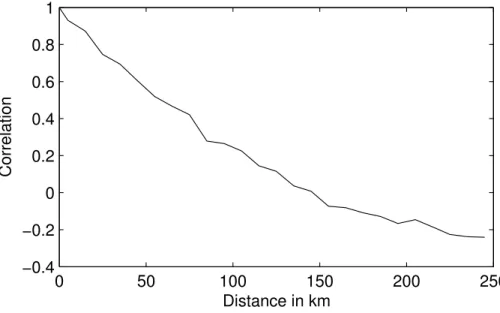
been subtracted. This correlation function is shown in Fig.2. The correlation length scale of the SST defined by the correlation threshold ofe−1∼0.37 is 80 km (the chosen threshold is based on correlation function of the typee−d /Lwhered is the distance). This is in agreement with both error length scales, since we can expect that the SST length scale is larger (but of the same magnitude) than the SST error length scale. 5

Both calibration methods for the correlation length of the observational error are thus not incoherent with the correlation length of the signal. Since in addition the analysed fields are very similar for both values and the error fields are not fundamentaly different (compare panels (c) and (d) of Fig. 3 with panels (a) and (b) of Fig. 4), no further optimisation seems necessary. Hence we present the results from the second 10

approach, based on the analysis error minimisation and leading to a clearer separation of the scales of noise (29 km) and signals (80 km). Note that the internal radius of deformation has a value of 4–7 km during winter in this region (e.g.,Barth et al.,2005) leading to an associated wavelength of the order of 25–44 km. The meanders of the Northern current exhibit a typical length scale of 30 km to 60 km (e.g.,Sammari et al., 15

1995).

In order to confirm the validity of our approach consisting in taking the error fields from OI as error fields for DINEOF, the RMS difference between SST estimations from OI and DINEOF should be smaller than this error estimation. The RMS difference between both fields is 0.17◦C and indeed smaller than the average error:

20

v u u t

1

mn

m

X

i=1

n

X

j=1

ǫ2_ij =0.24◦C. (54)

We also computed the difference between DINEOF SST (xr) and the OI SST (xr,(OI)) scaled by the error estimation:

yi j =

xr_{i j}₋x_ijr,(OI)2 ǫ2

i j

. (55)

(23)

OSD

3, 735–776, 2006

Title Page

Tables Figures

◭ ◮

Back Close

Full Screen / Esc

EGU

In 93% of the data points the scaled difference is lower than 1. This means that for the vast majority of the data points, the di_fference between both reconstructions is smaller than the error estimation. However, this analysis takes only the error variance into account. The error estimation method also provides the error covariance. This enables us to establish the significance of the di_fference between reconstructions knowing the 5

spatial correlation of the error. We assume that both reconstructions are a realisation of the Gaussian distributed random variable with possibly different means but the same covariances, i.e. the error covarianceE_{given in Eq. (}₃₈_):

xr

j ∼ N(m r

j,Ej), (56)

xOI

j ∼ N(m OI

j ,Ej), (57)

10

wherej is the temporal index for the image under consideration. The difference also follows a Gaussian distribution:

d_j ₌xr

j −x OI

j ∼ N(m r j −m

OI

j ,2Ej). (58)

In order to transform this distribution into a normal one, we introduce the matrix ˜S_:

˜

S₌ r

n

2C

−1/2

ΣN−1UNT_, ₍₅₉₎

15

which transforms the covariance matrix of the differenced_j _{into the identity matrix:}

˜

SE_jS˜T₌ 1

2IN. (60)

The transformed variable follows therefore:

z_j ₌Sd˜ _j _{∼ N}_{( ˜}S₍mr

j −m OI

j ),IN). (61)

We will examine if the difference between both reconstructions is significant to reject 20

the null-hypothesis (H0):

mr

j =m OI

(24)

OSD

3, 735–776, 2006

Title Page

Tables Figures

◭ ◮

Back Close

Full Screen / Esc

EGU

In this case we would accept the alternative hypothesis H1:

mr

j 6=m OI

j . (63)

Under the null-hypothesis, the transformed variablez follows a normal distribution.

z_j _{∼ N}₍₀_,I_N₎_. ₍₆₄₎

Now we can test if our sample z_j _{has a mean significantly di}_ff_{erent from zero. We}

5

compute the average ofz_j over all EOF modes and over time,z. This mean is smaller than the criticalzα/2value used in a two-sided z-test forα=0.05.

|z|pNn=0.93< zα/2=1.96. (65) This statistical test shows that the averaged difference between the OI reconstruction and the DINEOF reconstruction are not sufficiently large to be statistically significant. 10

The previous test measured the magnitude of the bias. We can also perform a test based on the L2-norm. Under the null-hypothesis the sum of the squared zi j follow

aχ2-distribution withNn=29 040 degrees of freedom. If this sum exceeds the critical value of 28 644, then the null-hypothesis must be rejected. But in our case, this value is again below this threshold:

15

X

i,j

z_{i j}2 =3703<28 644. (66)

where the z-values are summed over time and over EOF modes. Both tests show

that the null-hypothesis cannot be rejected. This does not prove, however, that the hypothesis H0 is true. If there is any difference in the reconstructionsmr

j andm OI j , then

the difference is so small that it could not be detected by the current sample. But the 20

fact that we are using a large sample of 2640 images (corresponding to 10 years of data) gives us confidence that if there is any difference between both reconstructions, it must be small. Therefore we conclude that the OI reconstruction and the DINEOF reconstruction are sufficiently close for the OI-derived estimation to be also a valid error estimation for the DINEOF reconstruction.

25

(25)

OSD

3, 735–776, 2006

Title Page

Tables Figures

◭ ◮

Back Close

Full Screen / Esc

EGU

6.4 Results

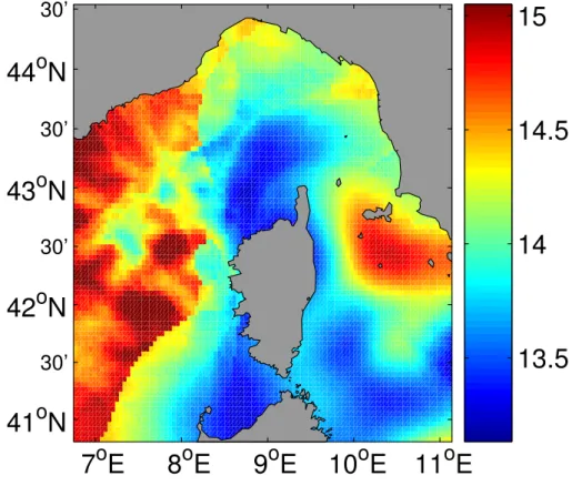
As an example of the reconstruction, Fig.3 shows a SST snapshot on 15 November

1998 (panel a). The central part of the Ligurian Sea and a fraction of the Tyrrhenian Sea are present in the observed SST. As one would expect, the estimated error standard deviation is the lowest in those regions. The error increases gradually and is highest 5

far away from the existing observations. Although the background error covariance is defined by global EOF modes and does therefore not include an explicit correlation length scale, the presented error estimation method was able to quantify the local effect of clouds on the error variance.

East of Corsica (approximatively at 42◦N and 9◦30′E) the error estimation is rela-10

tively high despite the presence of observations nearby. The SST standard deviation over the studied time period (Fig.5) is particularly high in this region. During summer this zone is warmer than e.g. the west coast of Corsica. The shallower depth of the east coast of Corsica shields this zone from the large-scale ocean current. This example shows that the error estimation takes also the variability of the field into account. 15

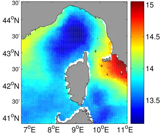
Although the Northern Current is covered by clouds in this snapshot, its SST signa-ture has been reconstructed by DINEOF (panel b) and the OI method (panel c) using the error covariance the EOFs computed by DINEOF. It is unlikely that an OI method using an isotropic and homogeneous error covariance would be capable of reconstruct-ing the Northern Current in a situation where very few data are available. To test this 20

possibility, we have made a comparison between the DINEOF reconstruction and an isotropic OI reconstruction on 30 December 2003. The cloudiness at and around this date is especially high, with some days with no data at all, which makes it appropriate for our purposes. Using a time window of 5 days, observations from the 26 December 2003, 27 December 2003, 30 December 2003 and 4 January 2004 are available for the 25

(26)

OSD

3, 735–776, 2006

Title Page

Tables Figures

◭ ◮

Back Close

Full Screen / Esc

EGU

length of 3 days are used.

The OI reconstruction (Fig.7) is degraded by the data on 26 December 2003, mostly in the western part of the Ligurian Sea. This image is the only one that presents a good data coverage, but the time difference between this image and the analised image is 5 days, and the SST on 30 December is notably colder than on 26 December. 5

The DINEOF reconstruction on 30 December 2003 (Fig.8) presents smoother values and a more realistic SST distribution on the western and northern Ligurian Sea. Both analysis are similar east of the Corsican island, in the Thyrrenian Sea, where most data are available. This example shows the ability of the global DINEOF analysis to produce better results than a standard isotropic OI reconstruction when only a few SST 10

observations are present. The EOF-based OI reconstruction on this date is similar to the reconstruction of Fig.8(image not shown).

6.5 Inter-annual variability

As an example of the DINEOF’s application we assess if the accuracy of the recon-structed SST is su_fficient to study inter-annual variability of the spatial averaged sea 15

surface temperature.

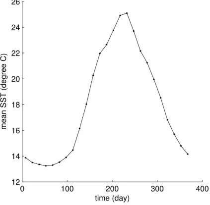
The average seasonal cycle has been computed from the reconstructed SST using all data from 1995 to 2005 filtered with 15-days cut-o_ff low pass filter (Fig. 9). The seasonal cycle shows an asymmetric behavior: while the mean temperature remains almost constant at the minimum temperature during January to March, the maximum 20

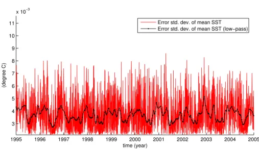
temperature is only reached during a short period of time during August. The deviations from this seasonal cycle are shown in Fig.10. The heatwave of 2003 affecting south Europe, in particular France, can be clearly seen from this time series. The error of the spatial mean SST (Fig.11) has been computed from Eq. (50). Since we can assume that the error of the seasonal cycle is negligible, the error estimate represents also the 25

expected error of the temperature anomaly of Fig.10. The expected error of the mean SST based on DINEOF is thus more than two orders of magnitude smaller than the inter-annual signal in SST of our studied domain. The reconstructed SST is therefore

(27)

OSD

3, 735–776, 2006

Title Page

Tables Figures

◭ ◮

Back Close

Full Screen / Esc

EGU

suitable to study inter-annual SST variability.

The expected error is highly variable in time, but the low-passed error estimate (cut-off frequency of 15 days) reveals a seasonal cycle in the error estimation. The re-construction has the highest error in winter and is about 25 % more accurate during summer. The seasonality of the error estimation is due to the cloud coverage. The 5

unfiltered error estimation correlates to 0.85 with the fraction of missing data. The cor-relation between the filtered error estimation and the filtered fraction of missing data is 0.92.

If we had taken the simple approach to calculate the mean temperature using only available data, we would have obtained another time-series. The difference between 10

the anomaly of the latter (compared to the same seasonal cycle) and our estimate of Fig. 10 has an rms value of 0.22◦C, much higher than the error estimate found in Fig. 11. Note that if we had also taken only the available data to calculate the confidence interval for the mean for the simple approach, we would have found an expected error on the mean of 0.012◦C. This is much lower than the actual error of 15

the simple estimate and yet higher than the error we get on the DINEOF analysis of the mean. Clearly, the DINEOF approach provides better estimates of the mean and narrower associated error bars.

7 Conclusions

We presented a method that allows to complement the cloud filling method DINEOF 20

with local error estimates. The approach uses the error estimates from optimal interpo-lation (OI), itself exploiting the covariance fields provided by DINEOF. Because of the factorisation of the covariance matrix also provided by DINEOF, OI can be performed as a least-square fit of EOF amplitudes, which drastically reduces computational re-quirements. The same approach can be exploited during the error calculations. 25

(28)

OSD

3, 735–776, 2006

Title Page

Tables Figures

◭ ◮

Back Close

Full Screen / Esc

EGU

the spatial means. It was shown that this approach allowed the isolation of interannual variability with very small error bars.

In the present case, the difference between the analysis provided by OI and DINEOF was shown to be smaller than the error fields, justifying the use of the error field for both analyses.

5

Should the difference be too large in some applications, the present method still allows to provide error estimates, but only for the OI. The latter, however, still benefits from the covariance factorization of DINEOF.

Another possibility would be to adapt DINEOF so as to include OI in the iterations, using the covariance from the EOFs under calculation, as the method of estimating 10

missing values. Such a hybrid approach would lead to a coherent set of EOFs, co-variance matrix and error fields. This approach was not yet implemented because in the cases we tested, the difference between OI and DINEOF were too small to justify the additional complexification. Probably a more important point to analyze for further improvement is the inherent hypothesis of the method that cloud coverage is uncorre-15

lated with the interpolated field. This can probably be justified for SST when clouds are not persistent but it is already more questionable for Chlorophyll which reacts rapidly to changes in insolation or storms associated with clouds. In this case, additional in-formation from scatterometers and in situ could probably help improve the detection of patterns of variability in a multivariate approach.

20

Acknowledgements. European projects MFSTEP (EVK3-CT-2002-00075), EUR-OCEANS

(Eu-ropean Network of excellence FP6 – Global change and ecosystems Contract number 511106) and Concerted action RACE (Communaut ´e Franc¸aise de Belgique) allowed to perform this work The National Fund for Scientific Research, Belgium is acknowledged for the financing of a supercomputer. D. Gomis made helpful suggestions on error estimates. The AVHRR

25

Oceans Pathfinder SST data were obtained from the Physical Oceanography Distributed Ac-tive Archive Center (PO.DAAC) at the NASA Jet Propulsion Laboratory, Pasadena, CA (http: //podaac.jpl.nasa.gov). This is MARE publication MAREXXX.

(29)

OSD

3, 735–776, 2006

Title Page

Tables Figures

◭ ◮

Back Close

Full Screen / Esc

EGU

Appendix A

Useful matrix identities

–

A₊UVT

-1

=A-1₋ A-1UI₊VTA-1U

-1

VTA-1 _(A1)

5

–

LTLLT₊_µ2I

-1

=LTL₊_µ2I

-1

LT _(A2)

provided the inverse matrix exists andI_{is an identity matrix (with 1 on the diagonal) of}

appropriate dimension.

References 10

Alvera-Azc ´arate, A., Barth, A., Rixen, M., and Beckers, J.-M.: Reconstruction of incomplete oceanographic data sets using Empirical Orthogonal Functions. Application to the Adriatic Sea, Ocean Modelling, 9, 325–346, 2005. 736,740,741,746

Astraldi, M., Balopoulos, S., Candela, J., Font, J., Gaci´c, M., Gasparini, G. P., Manca, B., Theocharis, A., and Tintor ´e, J.: The role of straits and channels in understanding the

char-15

acteristics of Mediterranean circulation, Prog. Oceanogr., 44, 65–108, 1999. 752

Barth, A., Alvera-Azc ´arate, A., Rixen, M., and Beckers, J.-M.: Two-way nested model of mesoscale circulation features in the Ligurian Sea, Prog. Oceanogr., 66, 171–189, 2005. 756

Barth, A., Alvera-Azc ´arate, A., Beckers, J.-M., Rixen, M., and Vandenbulcke, L.: Multigrid state

20

(30)

OSD

3, 735–776, 2006

Title Page

Tables Figures

◭ ◮

Back Close

Full Screen / Esc

EGU Beckers, J.-M. and Rixen, M.: EOF calculations from incomplete oceanographic data sets, J.

Atmos. Ocean Technol., 20, 1839–1856, 2003. 736,740

Bergant, K., Susnik, I., Strojan, M., and Shaw, A.: Sea Level Variability at Adriatic Coast and its Relationship to Atmospheric Forcing, Ann. Geophys., 23, 1997–2010, 2005. 737

Boyd, J., Kennelly, E., and Pistek, P.: Estimation of EOF expansion coefficients from incomplete

5

data, Deep Sea Res., 41, 1479–1488, 1994. 745

Daley, R.: Atmospheric Data Analysis, Cambridge University Press, 1991. 738

Emery, W. and Thomson, R.: Data analysis methods in physical oceanography, Pergamon, 1997. 739

Eslinger, D., O’Brian, J., and Iverson, R.: Empirical Orthogonal Function Analysis of

Cloud-10

Containing Coastal Zone Color Scanner Images of Northeastern North American Coastal Waters, J. Geophys. Res., 94, 10 884–10 890, 1989. 745

Evensen, G.: Sampling strategies and square root analysis schemes for the EnKF, Ocean Dynamics, 54, 539–560, 2004. 746

Gomis, D. and Pedder, M.: Errors in dynamical fields inferred from oceanographic cruise data:

15

Part I. The impact of observation errors and the sampling distribution, J. Mar. Syst., 56, 317–333, 2005. 736

Gomis, D., Ruiz, S., and Pedder, M.: Diagnostic analysis of the 3D ageostrophic circulation from a multivariate spatial interpolation of CTD and ADCP data, Deep Sea Res., 48, 269– 295, 2001. 736

20

Gunes, H., Sirisup, S., and Karniadakis, G.: Gappy data: To Krig or not to Krig?, J. Comput. Phys., 212, 358–382, 2006. 737

Kaplan, A., Kushnir, Y., Cane, M., and Blumenthal, B.: Reduced space optimal analysis for historical data sets: 136 years of Atlantic sea surface temperature, J. Geophys. Res., 102, 27 853–27 860, 1997. 745

25

Kondrashov, D., Feliks, Y., and Ghil, M.: Oscillatory modes of extended Nile River records (A.D. 622–1922), Geophys. Res. Lett., 3, L10 702, doi:10.1029/2004GL022156, 2005. 737 Larnicol, G., Le Traon, P. Y., Ayoub, N., and De Mey, P.: Mean sea level and surface

circu-lation variability of the Mediterranean Sea from 2 years of TOPEX/POSEIDON altimetry, J. Geophys. Res., 100, C12, 25 163–25 177, 1995. 752

30

Lawson, C. and Hanson, R.: Solving Least square problems, Prentice Hall, 1974. 745

Millot, C.: Circulation in the Western Mediterranean Sea, J. Mar. Syst., 20, 423–442, 1999. 752