Hydrol. Earth Syst. Sci., 17, 1241–1263, 2013 www.hydrol-earth-syst-sci.net/17/1241/2013/ doi:10.5194/hess-17-1241-2013
© Author(s) 2013. CC Attribution 3.0 License.
Geoscientiic
Geoscientiic
Hydrology and
Earth System
Sciences
Open Access
Theoretical framework to estimate spatial rainfall averages
conditional on river discharges and point rainfall measurements
from a single location: an application to western Greece
A. Langousis and V. Kaleris
Department of Civil Engineering, University of Patras, Patras, Greece Correspondence to:A. Langousis ([email protected])
Received: 22 October 2012 – Published in Hydrol. Earth Syst. Sci. Discuss.: 5 November 2012 Revised: 25 January 2013 – Accepted: 1 March 2013 – Published: 22 March 2013
Abstract.We focus on the special case of catchments cov-ered by a single rain gauge and develop a theoretical frame-work to obtain estimates of spatial rainfall averages condi-tional on rainfall measurements from a single location, and the flow conditions at the catchment outlet. In doing so we use (a) statistical tools to identify and correct inconsisten-cies between daily rainfall occurrence and amount and the flow conditions at the outlet of the basin; (b) concepts from multifractal theory to relate the fraction of wet intervals in point rainfall measurements and that in spatial rainfall aver-ages, while accounting for the shape and size of the catch-ment, the size, lifetime and advection velocity of rainfall-generating features and the location of the rain gauge in-side the basin; and (c) semi-theoretical arguments to assure consistency between rainfall and runoff volumes at an inter-annual level, implicitly accounting for spatial heterogeneities of rainfall caused by orographic influences. In an applica-tion study, using point rainfall records from the Glafkos river basin in western Greece, we find the suggested approach to demonstrate significant skill in resolving rainfall–runoff in-compatibilities at a daily level, while reproducing the statis-tics of spatial rainfall averages at both monthly and annual time scales, independent of the location of the rain gauge and the magnitude of the observed deviations between point rainfall measurements and spatial rainfall averages. The de-veloped scheme should serve as an important tool for the ef-fective calibration of rainfall–runoff models in basins cov-ered by a single rain gauge and, also, improve hydrologic impact assessment at a river basin level under changing cli-matic conditions.
1 Introduction
For many hydrological applications, such as calibration of rainfall–runoff models, estimation of river dischargesQ(t ) at the outlet of a basin and quantification of runoff extremes, one needs to calculate spatial averages of daily precipitation. A frequently used estimator for the spatially averaged rainfall intensityI (t )over a basin is
ˆ
I (t )=
s X
j=1
cjIj(t ), (1)
whereIj(t )is the average rainfall intensity on dayt at
lo-cationj= 1, ...,s inside the basin, andcj(j= 1, ...,s) are
strictly positive weighting coefficients that sum to 1. One can obtain cj(j= 1, ..., s) using a simple method based
on Thiessen polygons (Thiessen, 1911, and more recently, Eagleson, 1970; Shaw, 1983; Chow et al., 1988; Singh, 1992) or Kriging (Krige, 1951, and more recently Journel and Huijbregts, 1978; Isaaks and Srivastava, 1989; Banerjee et al., 2004; Press et al., 2007; Koutsoyiannis and Langousis, 2011), or alternatively apply equal weights. In the latter case cj= 1/sfor anyj. The accuracy of the estimator in Eq. (1)
in-creases with increasing numbersof the measuring locations inside the basin.
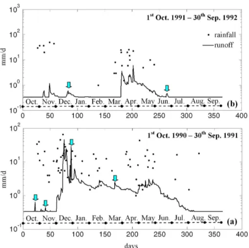
Fig. 1.Measured precipitation depths and daily river discharges per unit area of the basin at the location of the hydroelectric plant (HP, point A in Fig. 2) for the period 1 October 1990–30 September 1992. Vertical arrows indicate abrupt changes of the river discharge in the absence of rain.
Langousis (2005), Veneziano and Langousis (2005a) and Veneziano et al. (2006). The latter is an important issue for many catchments in Greece, and other countries in the Mediterranean region, which causes important problems in the calculation of annual water budgets and the calibration of hydrological models.
In what follows, we focus on the special case of catch-ments covered by a single rain gauge (i.e.j=s= 1). In this caseIˆ=I1=I and Eq. (1) approximates spatial rainfall
av-erages over the basin using rainfall measurements at a sin-gle location. This approximation has well-known limitations originating from the highly variable and lacunar character of rainfall fields (see Smith, 1993; Lovejoy and Schertzer, 1995; Veneziano and Langousis, 2010; Koutsoyiannis and Langousis, 2011, among others), which causes the process of spatial rainfall averages to differ significantly from that of point rainfall measurements; see e.g. Langousis (2005), Veneziano and Langousis (2005a), Veneziano et al. (2006), and Eleuch et al. (2010).
To prove this argument theoretically, it suffices to note that for spatially intermittent rainfall intensity fields and fi-nite sized catchments P[I (t ) >0|I (t )= 0]>0 and, there-fore, P[I (t ) >0]> P[I (t ) >0]. Note that the difference P[I (t ) >0]−P[I (t ) >0] increases with increasing catch-ment size.
The latter inequality highlights an important issue that emerges when approximating spatial rainfall averages over a catchment using point rainfall measurements. This is the un-derestimation of the fraction of wet intervals of the spatially averaged rainfall series which leads to incompatibilities be-tween rainfall occurrences and observed changes of the daily river runoff. Another issue concerns the observed imbalances in annual water budgets, caused by the underestimation of the fraction of wet intervals, as well as orographic influences.
outlet of the catchment to vary somewhat, but abrupt and intense changes of the river discharge should be associated with rainfall events. The vertical arrows in Fig. 1 indicate such changes in the absence of rain.
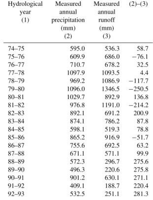
Table 1 shows annual precipitation depths and river dis-charges per unit area of the basin for the hydrological years (i.e. 1 October–30 September) 1974–1993. Note that for hy-drological years 1975–1976, 1978–1979, 1979–1980, 1981– 1982 and 1985–1986, the annual runoff volume is higher than that of precipitation. In addition, for all years on record, the readily available volume of water for evapotranspira-tion (ET) (i.e. precipitaevapotranspira-tion−runoff) is significantly lower than the ET-estimates reported in the literature for the wider region of the Glafkos catchment; see Voudouris (1995), Nikas (2004) and Mandilaras (2005). The latter are on the order of 500 mm per year. In the absence of physical in-dications for groundwater inflow from adjacent catchments (Kaleris and Ziogas, 2011), the aforementioned water imbal-ances can be attributed to incompatibilities between the his-torical point rainfall and runoff time series.
A rather straightforward way to correct the available point rainfall series and ensure consistency between annual rain-fall and river discharge volumes is to (1) calibrate a hydro-logical model using the historical rainfall and river discharge data, (2) calculate the difference1RO between measured and simulated annual runoffs, (3) adjust daily rainfall data using a multiplicative factor, calculated as the ratio between1RO and the measured annual precipitation depth, and (4) repeat steps 1–3 using the adjusted rainfall series; see Kaleris and Ziogas (2011). The suggested approach can be seen as an extension of the Parsons (or Sacramento) method developed in 1941 at the Corps of Engineers District Office in Sacra-mento (see US Army Corps of Engineers, 1941, and more re-cently Gilman, 1964) to determine mean annual precipitation in orographic areas. The Parsons method uses measurements of precipitation and runoff, as well as qualitative knowledge on soil and vegetation, to construct mean annual precipitation maps that minimize annual water imbalances in hydrological budgets.
While simple, the approach of Kaleris and Ziogas (2011) exhibits several intrinsic limitations. One is related to the fact that the hydrological model is calibrated using the original point rainfall records that are subject to adjustments. Hence, the level of the imposed correction and the quality and effec-tiveness of model calibration are strictly coupled.
Other, more theoretically oriented limitations relate to dif-ferences between the statistical characteristics of spatial rain-fall averages, which drive river flow and determine annual discharge volumes, and those of point rainfall measurements (see e.g. Eleuch et al., 2010). The latter can be seen as noisy observations of the former. For example, while a constant multiplicative correction factor may ensure consistency be-tween annual rainfall and river discharge volumes, it does not resolve incompatibilities between daily rainfall occurrence and flow conditions at the outlet of the catchment (see Fig. 1).
Table 1. Annual precipitation depths and river discharges per unit area of the basin at the location of the hydroelectric plant (HP, point A in Fig. 2) for the period 1 October 1974– 30 September 1993.
Hydrological Measured Measured (2)–(3) year annual annual
(1) precipitation runoff (mm) (mm) (2) (3)
74–75 595.0 536.3 58.7 75–76 609.9 686.0 −76.1 76–77 710.7 678.2 32.5 77–78 1097.9 1093.5 4.4 78–79 969.2 1086.9 −117.7 79–80 1096.0 1346.5 −250.5 80–81 1029.7 892.9 136.8 81–82 976.8 1191.0 −214.2 82–83 892.1 691.2 200.9 83–84 874.1 786.2 87.8 84–85 598.1 519.3 78.8 85–86 865.2 916.9 −51.7 86–87 755.6 692.5 63.2 87–88 671.1 571.1 99.9 88–89 572.3 296.7 275.6 89–90 496.3 220.6 275.8 90–91 901.2 630.1 271.1 91–92 409.1 188.7 220.4 92–93 532.5 251.1 281.3
In addition, such correction alters the distribution of rainfall intensities inside wet intervals without changing the fraction of dry intervals. In essence, the resulting time series do not resemble the structure of spatial rainfall averages. As previ-ously outlined, the latter exhibit a lower fraction of dry in-tervals relative to rainfall measurements at distinct locations inside the catchment.
A theoretically more appealing approach to ensure con-sistency between recorded rainfall and river discharges is to adjust point rainfall measurements to better resemble the sta-tistical structure of spatial rainfall averages at a daily level and, also, be consistent with the measured discharges at both daily and inter-annual levels.
In the next sections we propose a theoretical framework that uses rainfall data from a single rain gauge to obtain es-timates of spatial rainfall averages over a catchment condi-tional on the same- and previous-day discharges at the outlet. Consistency between the obtained estimates and observed runoffs is sought at both daily and inter-annual time scales.
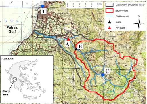
Fig. 2.The catchment of the Glafkos river in West Greece; see Sect. 2 for details.
hydrology, the quality and availability of water resources in space and time, and the sustainability of the natural environ-ment; see e.g. Kaleris et al. (2001) and Wilby et al. (2006). In Europe, the issues of water resource quality, availability and management have officially been stressed by the Water Framework Directive (WFD) 2000/60/EC of the European Parliament and of the Council on 23 October 2000.
The analysis is conducted using daily rainfall data and river discharges from the Glafkos river basin in western Greece. Temperature measurements do not enter the analy-sis, but they are used in Sect. 5 to obtain estimates of the actual evapotranspiration height in the basin. More details on the available data are given in Sect. 2.
Sections 3 and 4 present the theoretical framework of the suggested methodology. In Sect. 3 we develop a statisti-cal approach to identify and correct inconsistencies between daily rainfall occurrence and amount at the location of the rain gauge and the observed flow conditions at the outlet of the basin. Rainfall occurrence is checked using a statistical test based on the concept of linear reservoirs for river dis-charges (see Sect. 3.1), whereas daily rainfall intensities are modeled using a lognormal distribution with parameters that depend on the same- and previous-day discharge conditions at the outlet of the catchment (see Sect. 3.2).
As noted above, the fraction of wet intervals in spatial rain-fall averages differs from that observed in point rainrain-fall mea-surements. In Sect. 4 we use concepts from multifractal the-ory to relate the fraction of wet intervals in point rainfall, P1, to that observed in spatial rainfall averages, P1, while
accounting for the shape and size of the basin, the char-acteristics of rainfall-generating features (size, lifetime and
advection velocity vector), and the location of the rain gauge relative to the centroid of the basin (see Sect. 4.2). Since P1> P1(see above), several “dry” days in the record of point
rainfall measurements should be transformed to “wet”. Se-lection of those days is done conditional on the daily changes of the river discharge.
Section 5 focuses on the inter-annual consistency between rainfall measurements at a point and river discharges at the outlet of the basin and suggests a semi-theoretical approach to resolve water budget imbalances at an inter-annual level, implicitly accounting for spatial heterogeneities of rainfall (see Gilman, 1964; Smith, 1979; 1993 and Koutsoyiannis and Langousis, 2011 among others).
In Sect. 6 we apply and validate the efficiency of the method in resolving rainfall–runoff incompatibilities at both daily and annual time scales. A discussion of the main find-ings of this work as well as extensions and modifications of the suggested methodology for application to different cli-mates and catchment sizes are presented in Sect. 7.
2 Available data
Table 2. Physiographic properties of the study basin. The con-centration time tc has been calculated using the method of Watt and Chow (1985); see also Loukas and Quick (1996) and Dingman (2002).
Area 65.62 km2
Maximum elevation (a.m.s.l.) 1800 m Mean elevation (a.m.s.l.) 1060 m Average slope of the study basin 30 % Average slope of the main stream 6 % Length of the main channel 16 km Estimated concentration time 3.5 h
The hydroelectric plant (HP) is located downstream from the dam at a distance of about 2 km (point A in Fig. 2). Several physiographic properties of the study basin are summarized in Table 2.
2.1 Precipitation time series
Daily precipitation measurements are available by the Pub-lic Power Corporation (PPC) at three locations: (1) the dam (point B in Fig. 2), (2) the hydroelectric plant (HP) (point A in Fig. 2), and (3) the station of PPC at Moira (point C in Fig. 2). Station B is located at the outlet of the basin at an altitude of 340 m (a.m.s.l.), station A is located about 2 km downstream from station B at an altitude of 181 m, and sta-tion C is located close to the centroid of the basin at an alti-tude of 840 m (a.m.s.l.). For stations A and B, daily rainfall measurements are available for the period 1 October 1974 to 30 September 1993 (19 yr), whereas for station C for the period 1 October 1975 to 30 September 1994 (19 yr).
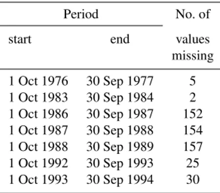
The available records at stations A (hydroelectric plant, HP) and B (dam) are complete, whereas the rainfall record at station C exhibits some missing values as shown in Table 3. For the period 1 October 1976 to 30 September 1993, the missing values have been completed by simple averaging of the corresponding daily rainfall measurements at stations A and B, whereas the period 1 October 1993 to 30 Septem-ber 1994, where no measurements are reported at stations A and B, was not included in the analysis.
During the wet period of the year (from November to April) the rainfall measurements at the Moira station were found to exhibit numerous small values in the range from 0.01–1 mm day−1. Since the accuracy of the rain gauge at the Moira station is on the order of 1 mm day−1(PPC, personal communication, 2012) and the Moira station is located in a forested area with significant vegetation, those values should be associated with dew and fog drip (occult precipitation) and were set to zero.
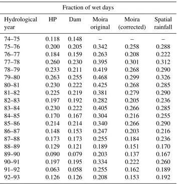
Tables 4 and 5 show annual rainfall depths and the frac-tion of wet days for the available historical rainfall records. One sees that (1) contrary to the original precipitation series at Moira the corrected ones exhibit lower wet-day fractions
Table 3.Number of missing values of daily rainfall measurements at station C (Moira).
Period No. of
start end values missing
1 Oct 1976 30 Sep 1977 5 1 Oct 1983 30 Sep 1984 2 1 Oct 1986 30 Sep 1987 152 1 Oct 1987 30 Sep 1988 154 1 Oct 1988 30 Sep 1989 157 1 Oct 1992 30 Sep 1993 25 1 Oct 1993 30 Sep 1994 30
Table 4.Annual rainfall totals for the observed, corrected and cal-culated rainfall series.
Annual rainfall totals (mm yr−1)
Hydrological Dam HP Moira Moira Spatial
year original (corrected) rainfall
74–75 771.7 595.0 – – –
75–76 762.5 609.9 1184.8 1174.6 1092.2
76–77 646.4 710.7 1071.7 1062.1 979.0
77–78 1163.5 1097.9 1667.5 1656.2 1557.7
78–79 1036.7 969.2 1328.1 1314.4 1258.9
79–80 1221.6 1096.0 1762.8 1746.5 1641.5
80–81 1178.3 1029.7 1709.9 1691.2 1588.6
81–82 1122.6 976.8 1579.0 1572.6 1482.6
82–83 974.2 892.1 1237.4 1229.7 1178.6
83–84 892.5 874.1 1307.7 1295.2 1214.7
84–85 667.3 598.1 917.6 906.9 859.0
85–86 937.9 865.2 1374.6 1361.0 1276.4
86–87 830.5 755.6 1068.9 1060.5 1014.5
87–88 764.3 671.1 987.2 969.8 928.7
88–89 632.0 572.3 670.3 662.9 656.7
89–90 504.7 496.3 718.3 704.2 664.3
90–91 941.0 901.2 1105.5 1086.0 1057.0
91–92 517.0 409.1 618.0 602.7 585.6
92–93 547.7 532.5 919.6 911.3 838.6
that are closer to those observed at different locations inside and outside the catchment (see Table 5) and that (2) the cor-responding correction affects minimally the annual rainfall totals (see Table 4).
For the period common to all stations (i.e. 1 October 1975 to 30 September 1993), we used the original precipita-tion data at staprecipita-tion B (dam) and the corrected ones at sta-tion C (Moira) to calculate spatial rainfall averages using the method of Thiessen polygons; see Tables 4 and 5. The weighting coefficients were found to be 0.2 for station B and 0.8 for station C.
Table 5.Fraction of wet days for the observed, corrected and calcu-lated rainfall series.
Fraction of wet days
Hydrological HP Dam Moira Moira Spatial
year original (corrected) rainfall
74–75 0.118 0.148 – – –
75–76 0.200 0.205 0.342 0.258 0.288
76–77 0.184 0.159 0.263 0.208 0.222
77–78 0.260 0.230 0.395 0.301 0.312
78–79 0.233 0.211 0.419 0.268 0.290
79–80 0.263 0.255 0.468 0.299 0.326
80–81 0.230 0.222 0.425 0.268 0.285
81–82 0.225 0.219 0.381 0.279 0.290
82–83 0.197 0.192 0.282 0.205 0.236
83–84 0.230 0.222 0.405 0.266 0.285
84–85 0.170 0.167 0.304 0.216 0.255
85–86 0.214 0.214 0.340 0.266 0.290
86–87 0.148 0.153 0.247 0.203 0.216
87–88 0.173 0.173 0.255 0.184 0.236
88–89 0.129 0.121 0.189 0.151 0.170
89–90 0.090 0.079 0.203 0.137 0.167
90–91 0.197 0.195 0.334 0.222 0.260
91–92 0.063 0.058 0.255 0.162 0.189
92–93 0.126 0.126 0.208 0.153 0.192
catchment (see above), obtaining results also for this station allows one to compare the estimated mean areal precipita-tion from staprecipita-tions B and C (using the method of Thiessen polygons), to rainfall products derived independently from station A using the suggested methodology.
2.2 River discharge time series
Daily discharge measurements at the outlet of the hydro-electric plant (point A in Fig. 2) are available from 1 Oc-tober 1974 onward. These measurements correspond to the mean daily river flow at the outlet of the catchment (dam), as the river water from the reservoir is led to the hydroelec-tric plant through a pipeline. In the case of very high river discharges, a portion of the river water entering the reser-voir is not used for energy production and flows downstream through the spillway of the dam. This portion of the river dis-charge is measured at the spillway. The mean daily disdis-charge is obtained as the sum of the daily water volume supplied to the hydroelectric plant and the daily water volume flowing out of the reservoir through the spillway of the dam.
The historical discharge series have been corrected to eliminate sudden and intense drops of the measured runoff caused by abrupt operations on the energy production unit. In addition, daily discharge measurements below 0.25 m3s−1 were found to exhibit irregular fluctuations during summer months, in the absence of rain. Those fluctuations relate to the observation accuracy of the water level in the dis-charge channel of the hydroelectric plant (PPC, personal communication, 2012) and were smoothed out by assigning
a minimum discharge value = 0.25 m3s−1. (Note that the Glafkos river is a perennial stream with non-zero base flow during all years on record.) Table 6 shows annual discharges, per unit area of the basin, for the historical years on record, using the original and corrected discharge series. One sees that the applied corrections affect minimally the annual wa-ter volumes.
2.3 Temperature time series
Daily mean temperatures are available from the stations of the Hellenic National Meteorological Service (HNMS) in Pa-tras (point T in Fig. 2) and Araxos (approximately 30 km west of the city of Patras; not included in the map). The Patras station is located at an altitude of 1 m (a.m.s.l.) with available data for the period 1 October 1982–30 Septem-ber 2000, whereas Araxos station is located at an altitude of 15 m (a.m.s.l.) and has been operating since 1 October 1974. When calculating the actual evapotranspiration in the basin (Sect. 5) for the period 1 October 1974–30 September 1982 (where no measurements are available at the Patras station), we use mean annual temperatures from Araxos corrected to account for the difference between the mean elevation of the catchment (1060 m a.m.s.l.; see Table 2) and the altitude of the station, using a pseudo-adiabatic lapse rate equal to 0.65◦C/100 m (see Table 7). For the period 1 October 1982– 30 September 1993 we use the daily mean temperatures recorded at the Patras station (the closest station to the basin), also corrected to account for the difference between the mean elevation of the catchment and the altitude of the station. As shown by Ziogas (2006), the daily mean temperatures mea-sured at Patras and Araxos are highly correlated (correlation coefficientR= 0.96) and one can combine those records to cover the whole period of the analysis.
3 A statistical approach to identify and resolve incompatibilities between daily rainfall measurements and river discharges
3.1 Checking rainfall occurrence using a theoretically based statistical model
DefineQ(t )to be the river discharge at the outlet of a basin on dayt, and denote byS(t )the subsurface storage on the same day. A simple theoretical model to approximate river discharges on dry days is that of a linear reservoir with zero inflow (see e.g. Chow, 1964; Lettenmaier and Wood, 1993):
Q(t )=αS(t ) dS(t )= −Q(t )dt
⇒Q(t )=Q(t−dt ) e−αdt, (2) whereα≥0 is a time constant. For dt= 1day, it follows from Eq. (2) that the ratio
ω(t )= Q(t )−Q(t −1) Q(t−1) =e
−α
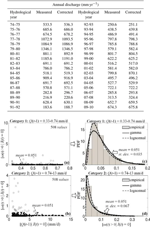
Fig. 3. (a, b)Scatter plots of the empirical ratios [ω(t ) >0|I (t )= 0], calculated using daily discharges and rainfall data from the hydroelectric plant (HP; point A in Fig. 2) for the period 1 October 1974–30 September 1993 (i.e. 19 yr, 1001 points) and split into 2 equally populated categories with respect to the previous-day river dischargeQ(t−1). Empty circles indicate values ofωfor which the null hypothesis of no rain over the catchment is rejected at the 5 % significance level; see main text.(c, d)Empirical histograms of the ratios (dots) in(a)and(b)
fitted by gamma (solid lines) and lognormal (dashed lines) distribution models.
Deviations from the model in Eq. (2) may cause the time constantαand consequently the ratioωto vary slowly with the previous-day dischargeQ(t−1).
Strictly speaking, in the absence of rain, positive values ofωare very likely not feasible, especially in Mediterranean basins. Hence, while small positive values (say on the order of 0.2–0.5) may be justified by snowmelt, variations of base flow and light rainfall occurrence at some ungauged part of the catchment, larger values ofωshould be associated with measurement errors or heavy rainfall at some ungauged part of the catchment.
Figures 3–5 show scatter-plots and empirical histograms of [ω(t ) >0|I (t )= 0] using daily river discharges and rain-fall depths measured at points A (HP) and B (dam) for the period 1 October 1974–30 September 1993 (19 yr) and C (Moira) for the period 1 October 1975–30 September 1993 (18 yr). The analysis has been conducted by (1) calculating the ratioω(t ) on days that appear as dry in the historical record of point rainfall measurements and (2) classifying the positive values ofωinton= 2 equally populated categories with respect to the previous-day river discharge Q(t−1). Classification is done in order to study how the statistics of ωdepend onQ(t−1); see below. The solid and dashed lines on the right panels of Figs. 3–5 correspond to gamma and lognormal distribution models, respectively, fitted directly to the empirical ratios using the method of moments. The fitting
procedure is suited to account for and remove irregularly high values ofω, as follows.
1. For each category of previous-day river discharges, Q(t−1), one removes a single value ofωand fits the corresponding theoretical distribution model to the re-mainder values.
2. One checks whether the removed value can be classi-fied as an outlier at a certain level of significance β (e.g.β= 5 %)
3. One repeats steps 1 and 2 for all values of ω in the category.
4. One fits the corresponding theoretical distribution model to those values ofωidentified as non-outliers. One sees that, independent of the category of the previous-day dischargeQ(t−1), both gamma and lognormal distri-bution models fit equally well the data. In what follows, we choose to modelωusing a lognormal distribution with pa-rameters that depend onQ(t−1).
Table 6. Annual discharges, per unit area of the basin, for the original and corrected runoff series for the period 1 October 1974 to 30 September 2010.
Annual discharge (mm yr−1)
Hydrological Measured Corrected Hydrological Measured Corrected
year year
74–75 533.5 536.3 92-93 250.6 251.1 75–76 685.6 686.0 93-94 438.5 439.8 76–77 674.5 678.2 94-95 486.9 491.4 77–78 1072.9 1093.5 95-96 797.8 798.3 78–79 1084.9 1086.9 96-97 785.8 788.8 79–80 1346.1 1346.5 97-98 579.1 582.4 80–81 881.1 892.9 98-99 801.7 804.5 81–82 1185.6 1191.0 99-00 622.2 625.2 82–83 691.1 691.2 00-01 516.2 517.0 83–84 786.0 786.2 01-02 581.4 582.0 84–85 518.1 519.3 02-03 799.8 870.1 85–86 909.4 916.9 03-04 495.7 496.2 86-87 691.7 692.5 04-05 527.7 529.9 87–88 570.8 571.1 05-06 722.1 722.2 88–89 282.8 296.7 06-07 285.8 293.8 89–90 216.9 220.6 07-08 313.5 324.4 90–91 628.4 630.1 08-09 652.7 659.5 91–92 183.6 188.7 09-10 674.3 675.8
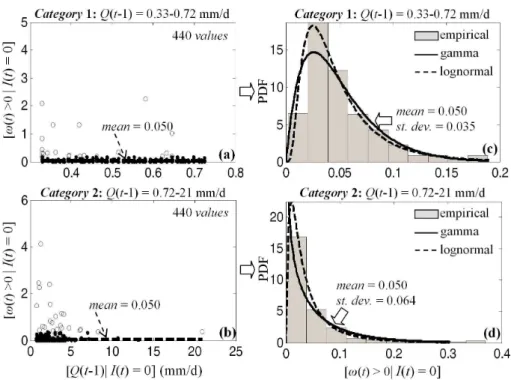
Fig. 4.Same as Fig. 3 but using daily rainfall intensities from the location of the dam (point B in Fig. 2) for the period 1 October 1974– 30 September 1993 (i.e. 19 yr, 1016 points).
rainfall measurements and changes of the river discharge at the outlet of the basin. The left panels of Figs. 3–5 show scatter-plots ofωfor different categories of river discharges and rainfall data sets. The empty circles indicate (outlier)
values ofωfor which the null hypothesis of no rain over the catchment is rejected at the 5 % significance level.
Fig. 5.Same as Fig. 4 but using daily rainfall intensities from the location of Moira (point C in Fig. 2) for the period 1 October 1975– 30 September 1993 (i.e. 18 yr, 880 points).
Table 7. Mean annual temperatures at the Glafkos catchment (mean elevation: 1060 m a.m.s.l.) for the period 1 October 1974 to 30 September 1993.
Hydrological Mean year annual temperature (◦C)
74–75 9.83
75–76 9.73
76–77 10.60
77–78 9.95
78–79 10.43
79–80 9.53
80–81 9.98
81–82 9.86
82–83 10.33 83–84 10.10 84–85 10.93 85–86 11.04 86–87 10.51 87–88 11.37 88–89 10.63 89–90 11.01
90–91 9.83
91–92 9.35
92–93 10.69
see Figs. 3–5) and a variance that increases with increasing Q(t-1). The latter increase is physically justified since larger values ofQ(t−1) indicate intense discharge conditions that can more easily produce extreme runoffs. An additional ob-servation is that, independent of the category of previous-day dischargeQ(t−1), the statistics of the values ofωthat sat-isfy the null hypothesis do not depend on the rainfall data set. This highlights the robustness of the statistical method in identifying and eliminating incompatibilities between daily rainfall occurrences and changes in the river runoff, while maintaining those values ofωthat share similar statistics. In the next section we focus on wet days and model daily rain-fall intensities using a lognormal distribution with parame-ters that depend on the same- and previous-day discharge conditions at the outlet of the catchment.
3.2 Statistical model for daily rainfall intensities conditioned on river discharges
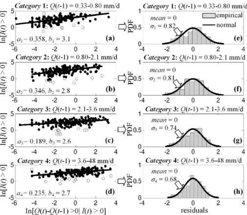
Fig. 6. (a–d)Plots of logarithmically transformed daily rainfall intensities on wet days, ln[I (t ) >0], as a function of the observed change of the river discharge ln[Q(t )−Q(t−1)>0] for 4 (four) equally populated categories of the previous-day river dischargeQ(t−1). The analysis has been conducted using daily discharges and rainfall data from the location of the hydroelectric plant (HP; point A in Fig. 2) for the period 1 October 1974–30 September 1993 (i.e. 19 yr, 656 points). Estimates of the parametersaj andbj (j= 1, ..., 4) in Eq. (4) have
been obtained by least-squares fitting of the empirical values. Empty circles correspond to outliers of the log–log linear regression at 5 % significance level.(e–h)Empirical histograms of the residuals of the log–log linear regression in(a–d)fitted by a normal distribution model with zero mean and variance (σj)2= Var[Vj]; see Eq. (4).
A way to proceed in this direction is to develop re-lationships that describe how the statistics of daily rain-fall intensities vary with indicator variables representative of the flow conditions at the outlet of the basin. For the same data sets used in Figs. 3–5, Figs. 6–8 show plots of the logarithmically transformed daily rainfall intensities, ln[I (t ) >0], on wet daystas a function of the observed pos-itive change of the river discharge [Q(t )−Q(t−1)>0] for different categories of the previous-day dischargeQ(t−1). Dependence of the statistics of [I (t ) >0] onQ(t−1) and [Q(t )−Q(t−1)>0] is physically justified, since (a) larger values of Q(t−1) indicate intense discharge conditions that more easily produce extreme runoffs and, consequently, larger values of the difference Q(t )−Q(t−1), and since (b) larger values of the differenceQ(t )−Q(t−1) are as-sociated with more-intense rainfall events.
The solid lines on the left panels of Figs. 6–8 are best fits of Eq. (4) (see below) to the empirical data using the method of least squares,
ln[I (t ) >0|Q(t )−Q(t −1) >0]
=ajln[Q(t )−Q(t −1) >0] +bj +Vj,
j =1,2, ..., m. (4)
aj andbj in Eq. (4) are parameters that depend on the
cat-egoryj of the previous-day dischargeQ(t−1), andVj is a
zero-mean random error term that is stochastically indepen-dent from the variable [Q(t )−Q(t−1)]. Calculation of the parametersajandbj proceeds as follows.
1. One identifies the wet days (i.e. I (t ) >0) in the his-torical record for whichQ(t )−Q(t−1)>0. For those days, the measured rainfall intensitiesI (t )and the ob-served changes of the river runoffQ(t )−Q(t−1) are ranked based on the previous-day river flowQ(t−1) and split intom= 4 equally populated categories. 2. The coefficientsajandbj, as well as the residuals of the
regressionvj,k,k= 1, 2, ..., are calculated separately for
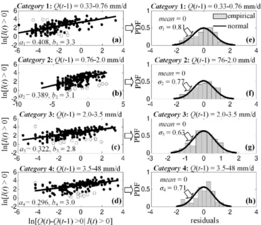
Fig. 7.Same as Fig. 6 but using daily rainfall intensities from the location of the dam (point B in Fig. 2) for the period 1 October 1974– 30 September 1993 (i.e. 19 yr, 641 points).
3. To put residuals at a comparable scale, one divides them by an estimate of their standard deviation (see Chatterjee and Hadi, 1986, Eq. 13) that is independent of their value. As shown on the right panels of Figs. 6–8, independent of the categoryj of the previous-day river dischargeQ(t−1), the residuals of the log–log linear regression are well approximated by a normal distribu-tion with zero mean and varianceσj2 that depends on the categoryj. Hence, the resulting samples of the stan-dardized residuals should be well approximated by a Studentt distribution withNj−p−1 degrees of
free-dom (df), whereNjis the sample size of categoryj and
p= 2 is the number of parameters of the log-linear re-gression; see e.g. Belsley et al. (1980), Velleman and Welsch (1981), Atkinson (1981) and Chatterjee and Hadi (1986).
4. For a certain level of significanceβ(e.g., 5 %), one uses the standardized residuals from step 3 and the Studentt theoretical distribution model to identify outliers of the initial regression (see empty circles on the left panels of Figs. 6–8), remove them, and then obtain a new set of coefficientsaj andbj.
Figure 9 shows how the empirical estimates of the param-etersaj andbj in Eq. (4) and the error standard deviation
σj vary with the previous-day dischargeQ(t−1). The solid
lines are least-squares fits to the empirical values. One sees that botha andb decrease log–log linearly with increasing Q(t−1). This is physically expected since larger values of Q(t−1) correspond to more-intense discharge conditions, where large changes of the river discharge between two se-quential daysQ(t )−Q(t−1) can also be caused by less in-tense rainfall events.
Two additional observations one makes are that, indepen-dent of the rainfall data set, the empirical distribution of the residuals of the regression in Eq. (4) is close to normal with variance that does not depend on the previous-day discharge Q(t−1). The first observation is in accordance with the find-ings of many studies suggesting the use of a lognormal dis-tribution model for rainfall intensities; see e.g. Kedem et al. (1990a,b, 1997), Shimizu (1993), Cheng and Qi (2002), Cho et al. (2004), Veneziano and Langousis (2005a,b), Shoji and Kitaura (2006), Veneziano et al. (2006, 2007), Suhaila and Jemain (2007), Langousis and Veneziano (2007), and Langousis et al. (2009). The second observation is physically justified since the variability of rainfall should not depend on the previous-day flow conditions.
Fig. 8.Same as Fig. 7 but using daily rainfall intensities from Moira station (point C in Fig. 2) for the period 1 October 1975–30 Septem-ber 1993 (i.e. 18 yr, 695 points).
µlnI=E[ln{I (t ) >0|Q(t )−Q(t−1) >0, Q(t−1)}]
=aQ(t−1)ln[Q(t )−Q(t−1) >0] +bQ(t−1)
(σlnI)2=Var[ln{I (t ) >0|Q(t )−Q(t−1) >0, Q(t−1)}]
=c2=const., (5)
whereµlnI and (σlnI)2are the mean and variance of the
as-sociated normal distribution,aQ(t−1)andbQ(t−1)can be
cal-culated from the equations in Fig. 9 based on the previous-day dischargeQ(t−1), andcis a constant independent of Q(t−1). Equation (5) is used to assign synthetic rainfall in-tensity values to (1) days identified with inconsistencies be-tween point rainfall measurements and flow conditions at the outlet of the catchment (see empty circles in Figs. 3–8) and to (2) additional wet days when adjusting point rainfall mea-surements to better resemble the fraction of wet intervals in spatial rainfall averages; see next section.
4 Using concepts from multifractal theory to relate the fraction of wet intervals in point rainfall to that in spatial rainfall averages
DefineI (t )to be the spatially averaged daily rainfall depth over a catchment on day t, and denote by I (t ) the daily
rainfall depth at a certain locationj inside the basin on the same day. From total probability theorem one has
P[I (t ) >0] =1−P0 =P[I (t ) >0|I (t ) >0](1−P0)
+P[I (t ) >0|I (t )=0]P0, (6) whereP0=P[I (t )= 0] andP0=P[I (t )= 0], and from
con-ditional probability theorem one has
P[I (t ) >0|I (t )=0] = 1−P0
P[I (t )=0|I (t ) >0]
P0
. (7) By combining Eqs. (6) and (7) one obtains
P0=1−
δ (1−P0)
1−P[I (t )=0|I (t ) > 0], (8) whereδ=P[I (t ) >0|I (t ) >0].
It follows from the definition of spatial rainfall averages that whenj is located inside the catchment or at the basin divide,δ= 1. Thus,
P0=1−
(1−P0)
Fig. 9.Plots of the parametersaj andbj (j= 1, ..., 4) in Eq. (4),
and the error standard deviationσj= Var[Vj]0.5as functions of the
previous-day river dischargeQ(t−1), for the rainfall data sets used in Figs. 6–8. Lines correspond to least-squares (LS) fits to the em-pirical values.
Table 8.Categories of precipitation areas and their characteristics; adapted from Langousis (2005).
Type Area,Amax Linear Lifetime, Advection
dimension, dL velocity,
Lmax vad
small areas ∼10 km2 3 km <30 min
30–50 km h−1 small 100–400 km2 10–20 km ∼1 h
mesoscale areas
large 103–104km2 30–100 km several
20–40 km h−1 mesoscale hours
areas
synoptic >104km2 >100 km ≥1 day scale areas
the probabilityP[I (t )= 0|I (t ) >0] in Eq. (9) (i.e. the prob-ability that it does not rain at locationj given that it rains inside the basin) to the shape and size of the catchment and the characteristics of storms.
4.1 Borrowing concepts from multifractal theory to approximate Eq. (9)
Rainfall-generating features evolve in time and advect in space. Hence, rain gauge rainfall measurements are repre-sentative estimates of spatial rainfall averages over an indica-tive areaA0, which depends on the characteristics (size,
life-time, advection velocity vector, etc.) of rainfall-generating features. Suppose now that spatial rainfall is homogeneously multifractal below some maximum area Amax∝(Lmax)2,
whereLmax is the linear spatial dimension of the
rainfall-generating features; see below. In this case (see e.g. Schertzer and Lovejoy, 1987; Gupta and Waymire, 1993; Veneziano, 1999; Veneziano and Langousis, 2010),
I (t )=d YrI (t ), (10)
where =d denotes equality in all finite dimensional dis-tributions, Yr is a unit mean random variable
indepen-dent ofI (t )with parameters that depend on the resolution r=A/A0< Amax/A0, and A is the area of the catchment.
Estimates ofAmaxandLmaxare summarized in Table 8; see
e.g. Austin and House (1972), Orlanski (1975), Veneziano and Langousis (2005a), and the review in Langousis (2005). For subtropical regions where rainfall is mainly dominated by stratiform formations, an average value ofLmaxis on the
order of 50–100 km or more.
For spatial rainfall fields, a commonly used assumption to model the alternation of wet and dry regions is the use of a beta-lognormal distribution model for Yr (Schertzer
and Lovejoy, 1987; Over and Gupta, 1996; Schmitt et al., 1998; Langousis and Veneziano, 2007; Langousis et al., 2009). In this case, Yr has a concentrated mass
normal distribution with mean µ= -Clnlnr and variance
σ2= 2Clnlnr. The parameterCβ controls the alternation of
wet and dry intervals inside Amax, whereas Cln is
respon-sible for the intensity fluctuations inside rainy regions; see e.g. Langousis et al. (2009).
Several empirical studies (Over and Gupta, 1996; Kundu and Bell, 2003; Deidda et al., 2004, 2006; Gebremichael et al., 2006) have shown that spatial rainfall scales in an approximately multifractal way for areas A from 4– 4000 km2, with values ofCβ that vary from 0.2–0.3 for areas
4 km2≤A≤256 km2(Kundu and Bell, 2003) and from 0.3– 0.6 for 256 km2≤A≤4096 km2 (Over and Gupta, 1996; Deidda et al., 2004, 2006; Gebremichael et al., 2006); see also the review in Veneziano and Langousis (2010). Based on the multifractal model in Eq. (10), one obtains
P[I (t )=0|I (t ) >0] =P[Yr=0]=1−r−Cβ, (11)
and Eq. (9) simplifies to P0 =1−
1−P0
r−Cβ . (12)
Given the aforementioned Cβ ranges, for small
catch-ments (i.e. 4 km2≤A≤256 km2, as is the case for the Glafkos basin) the value of Cβ can be set to a
con-stant ≈0.25. For medium- and large-sized catchments (i.e. 256 km2≤A≤4096 km2) the value ofCβ can be taken
to increase log–log linearly withAfrom 0.3–0.6. In what fol-lows, we propose a theoretical approach to obtain estimates of the resolutionrin Eq. (12).
4.2 Linking the resolutionrin Eq. (12) to the shape
and size of the catchment and the characteristics of storms
Defineθto be the direction of motion of rainfall-generating features (see Fig. 10), and denote byLcthe characteristic
lin-ear dimension of the catchment. For regularly shaped catch-mentsLc∝
√
A, whereas for highly elongated catchments Lc can be taken proportional to their largest linear
dimen-sion (Veneziano and Langousis, 2005a). As rainfall features propagate in space and evolve in time, a rain gauge located at point8samples rainfall along lineε(see Fig. 10). Note, however, that only line segment BŴ=x(θ )falls inside the basin. Consequently, for a storm moving along line ε, the characteristic linear sampling dimension of the rain gauge is
L(z)=min [x(θ ), vaddL], (13)
wherez= [θ,vad,dL]T is the vector of meteorological
vari-ables that characterize the storm, and vad and dL are the
advection velocity and lifetime of rainfall-generating fea-tures. Indicative ranges of values for vad and dL for
dif-ferent types of rainfall-generating features are given in Table 8; see Austin and House (1972), Orlanski (1975), Martin and Schreiner (1981), Kawamura et al. (1996), Deidda (2000), Veneziano and Langousis (2005a), and the review in Langousis (2005).
Fig. 10.Schematic illustration of the variables in Eq. (13), for a storm moving over a catchment at directionθ; see main text for details.
Equation (13) directly accounts for the effects of (a) the lo-cation of the rain gauge8inside the basin and (b) the lifetime dLand advection velocityvadof rainfall-generating features
on the characteristic sampling lengthL. In the case when the joint distributionfz(z)of the vectorz= [θ,vad,dL]T of
mete-orological variables is known or can be calculated from data, the expected linear sampling dimension of rain gauge8is obtained as
L= Z
allz
fz(z) L(z)dz. (14)
Examples of the calculation of similar expectations can be found in Langousis and Veneziano (2009), for the special case of tropical cyclones.
In the case when no meteorological data are available, one can assume a uniform distribution forθ in the interval [0, 2π], estimate dL from rainfall data as the average duration
of wet periods, and usedL to obtain a value for vad from
Table 8. Under these assumptions, Eq. (14) reduces to
L= 1 2π
2π Z
0
L (θ, vad, dL)dθ, (15)
whereL(θ,vad,dL)is given by Eq. (13). The resolutionrin
Eq. (12) is calculated asr= (A/A0) = (Lc/L)2, whereLcan
be obtained from Eqs. (14) or (15).
In Appendix A, we derive an analytical expression for Eq. (15) for regularly shaped catchments approximated as discs with diameter equal to their characteristic linear dimen-sionLc. Table 9 shows estimates of dL,L andr for
Table 9.Estimates of the average lifetime of rainfall features,dL, the average sampling length, (L) (see Eqs. 15 and A.3), and the res-olutionr(see Eq. 12), for locations A (HP), B (dam) and C (Moira); see Fig. 2. The last row of the table shows estimates of the inter-annual multiplicative correction factor obtained from Eq. (21).
Variable HP Dam Moira (181 m a.m.s.l.) (340 m a.m.s.l.) (840 m a.m.s.l.)
dL 1.96 days 1.97 days 2.06 days
Lc 9.14 km 9.14 km 9.14 km
L 5.82 km 5.82 km 9.14 km
r 2.47 2.47 1
h 1.16 1.08 0.86
(dam) are taken to be located approximately at the basin di-vide (i.e. the circumference of the disc; see Eq. A.3 in Ap-pendix A), and point C (Moira) at the centroid of the basin (i.e. the center of the disc). The resolutionrin Table 9 is used in Eq. (12) withCβ= 0.25 (see discussion under Eq. 12) to
calculate the number of additional wet days, needed in each month of the corrected time series (obtained in Sect. 3), to match the expected fraction of wet intervals in spatial rainfall averages. Additional wet days are prescribed starting from the largest value of the ratioωin each month of the record and moving to smaller values till either the number of addi-tional wet days is reached orω≤0.
5 Multiplicative correction for the annual rainfall depth
In Sect. 3 we developed a methodology to identify and re-solve incompatibilities between daily rainfall measurements I (t )at a point and river dischargesQ(t )at the outlet of the catchment, and in Sect. 4 we used concepts from multifractal theory to relate the fraction of wet intervals in point rain-fall to that in spatial rainrain-fall averages. In this way we cor-rected the record of point rainfall measurementsI (t )for in-compatibilities with river discharges at the outlet of the basin and, also, adjusted the resulting rainfall time series to exhibit the fraction of dry days outlined by multifractal theory for spatial rainfall averages,I (t ), over the catchment. This was done without altering the distribution of daily rainfall inten-sities on wet days (i.e. [Iadj(t )|Iadj(t ) >0]
md
=[I (t )|I (t ) >0], whereIadj(t )denotes the adjusted rainfall time series and
md
=
denotes equality of the marginal distributions).
Maintaining the same marginal distribution for point rain-fall measurements and spatial rainrain-fall averages on wet days would correspond to a spatially homogeneous rainfall in-tensity field. However, orographic effects might cause the distribution of spatial rainfall averages to deviate somewhat from that of point rainfall measurements. Several studies (see Pathinara and Herath, 2002; Badas et al., 2005; and Deidda et al., 2006) have shown that orography does not affect the statistical structure of rainfall time series (i.e. alternation of
Fig. 11.Correction factorwfor the actual evapotranspiration ETact calculated for flat catchments, as a function of the mean slope of the basin and its orientation (N: north, S: south, E: east; W: west); adapted from DVWK (1996).
wet and dry intervals, fraction of dry days, etc.) and, hence, rainfall at different elevations can be modeled by multiplying a spatially homogeneous rainfall intensity field by a smooth increasing function of the elevation; see Badas et al. (2005) and the review in Veneziano and Langousis (2010). This is equivalent to multiplying the adjusted rainfall intensity se-ries,Iadj(t ), by a constant multiplicative correction factorh.
In this case,
I (t )≈ ˆd I (t )=h Iadj(t ), (16)
whereIˆ is the suggested estimate for spatial rainfall and≈d
denotes approximate equality in distributions. In what fol-lows, we propose a semi-theoretical approach to estimateh in the absence of rainfall measurements at multiple locations inside the catchment.
DefineVl to be the annual rainfall volume reaching the
catchment in yearl= 1, 2, ..., and denote by ROl the annual
river discharge volume at the outlet of the basin in the same year. In the absence of groundwater inflows from adjacent catchments (see Introduction), the water budget equation is written, at an annual time scale, as
Vl =ROl +wETact,lA+1Sl, l=1, 2, ..., (17)
whereAis the area of the basin, ETact,lis the actual annual
evapotranspiration height in yearl for a flat catchment (see Eq. 18 below),wis a correction factor that accounts for the effects of the mean slopeJ of the catchment and its orien-tationϕon ETact (see below), and1Sl is the change in the
subsurface storage in yearl.
Figure 11 shows how the correction factorwvaries withϕ andJ. For the catchment of the Glafkos river, which exhibits a significant mean slope of about 30 % (see Table 2) facing northwest,w≈0.8.
Estimates of ETact can be obtained using semi-empirical
P and the mean annual temperatureT or the potential evapo-transpiration ETpot; see e.g. Shaw (1983). The latter is a
func-tion ofT. To check consistency of different actual evapotran-spiration models (e.g. Pike and Turc), we calculated ETact
using precipitation measurements from stations A, B and C and the temperature time series available for the catchment (see Sect. 2.3 and Table 7). We found that, for all years on record, the relative differences between different evapotran-spiration models are below 5 % and, hence, selection of a specific evapotranspiration model does not affect results. In what follows, we use the Turc model to estimate ETact,
ETact =P
0.9+
P
300+25T +0.05T3 !2
−1/2
, (18)
since it does not require separate calculation of the potential evapotranspiration.
Summing Eq. (17) over the recorded yearsl= 1, 2, ...,n, one obtains
n X
l=1
Vl = n X
l=1
ROl +w A n X
l=1
ETact,l+ n X
l=1
1Sl. (19)
Assuming that the catchment does not exhibit over-year de-pletion of the available water resources, the annual changes in the subsurface storage should balance out over the years. In this case
n P
l=1
1Sl= 0, and Eq. (19) reduces to
n X
l=1
Vl = n X
l=1
ROl +w A n X
l=1
ETact,l. (20)
Using Eq. (20), an estimate of the multiplicative correction factorhcan be obtained as
h=
n X
l=1
Vl
n
X
l=1
A Padj,l= n X
l=1
ROl
n
X
l=1
A Padj,l
+w
n X
l=1
ETact,l
n
X
l=1
Padj,l, (21)
wherePadj,l is the annual rainfall depth in year l= 1, ...,n
calculated using the adjusted point rainfall seriesIadj, and
ETact,lis calculated from Eq. (18) usingPadj,l. Table 9 shows
estimates of the multiplicative correction factorhusing rain-fall data from stations A, B and C. One sees that the correc-tion factors for locacorrec-tions A (h= 1.16) and B (h= 1.08) are larger than 1, whereas for location C (h= 0.86) it is below 1. This means that stations A and B underestimate annual rain-fall volumes (as noted in the Introduction and shown in Ta-ble 1), whereas station C overestimates them. The observed differences between the annual rainfall volumes measured at locations A, B and C are highly associated with the intense topography of the catchment, with more than 1500 m alti-tude change in less than 10 km. This is further justified by
the fact that the inter-annual multiplicative correction factor hdecreases with increasing elevation (see Table 9), as larger altitudes are associated with higher annual precipitation vol-umes; see e.g. Gilman (1964), Smith (1993) and Badas et al. (2005).
6 Model application and validation
To illustrate the use of the statistical framework presented in Sects. 3–5, Fig. 12 shows a realization of the estimated spa-tial rainfall series,Iˆ (see Eq. 16), obtained using point rain-fall measurements from station A (hydroelectric plant, HP) for the period 1 October 1990–30 September 1992 (same pe-riod as in Fig. 1), as well as daily discharges per unit area of the basin (solid lines) at the catchment outlet (point A in Fig. 2). Dots correspond to measured rainfall depths, empty circles to synthetic rainfall intensities assigned to dry days in-compatible with observed discharges at the 95 % confidence level (see Sect. 3.1 and empty circles in Fig. 3), triangles to synthetic rainfall intensities that substitute the outlier values (empty circles) in Fig. 6 (see Sect. 3.2), and diamonds to syn-thetic rainfall intensities assigned to additional wet days so that the resulting series match the fraction of wet intervals in spatial rainfall averages predicted by multifractal theory (see Sect. 4). Synthetic rainfall intensities are simulated ran-domly using a lognormal distribution model with parameters obtained from Eq. (5) and Fig. 9a. In addition, all rainfall values have been multiplied by a correction factorh= 1.16 (see Sect. 5 and Table 9) to account for the effects of spatial heterogeneity of rainfall on the annual water budgets.
Direct comparison of Figs. 1 and 12 shows good cor-respondence between observed changes of the river dis-charge and synthetic rainfall occurrence, with synthetic rain-fall events located inside wet periods of the year. Hence, ar-tificial interruptions of prolonged dry periods are avoided. This is an important attribute of the suggested approach, since it respects the seasonal character (see e.g. Langousis and Koutsoyiannis, 2006) and the clustered nature of rain-fall; see LeCam (1961), Waymire and Gupta (1981a,b,c) and the review in Koutsoyannis and Langousis (2011).
Fig. 12.Observed (dots) and simulated (empty circles, triangles and diamonds) daily rainfall intensities at the location of the hydroelectric plant (HP, point A in Fig. 2) for the period 1 October 1990–30 September 1992 (same period as in Fig. 1); see main text for details.
to point rainfall measurements from each location. Spatial rainfall averages (see Sect. 2.1) are used for validation pur-poses only, and do not enter the analysis at any step.
One sees that point rainfall measurements (dotted lines) from locations A (HP) and B (dam) exhibit lower monthly means and standard deviations relative to those of spatial rainfall averages (solid lines) (see Figs. 13 and 14), whereas point rainfall measurements from location C (Moira) slightly overestimate them (see Fig. 15). In addition, the fraction of dry intervals in point rainfall measurements is, in all cases, higher than that observed in spatial rainfall averages (for a justification, see Sect. 1).
Contrary to point rainfall measurements, the estimated rainfall intensities (dashed-dotted lines) reproduce well the statistics of spatial rainfall averages at a monthly time scale, independent of the location of the rain gauge, and the magni-tude of the observed deviations between point rainfall mea-surements and spatial rainfall averages (see Figs. 13–15). The same is true, also, at an annual level.
To illustrate this, Fig. 16 shows annual rainfall totals, yearly standard deviations, and the fraction of dry days in
different years, for the same rainfall series used in Fig. 13. One sees that, contrary to point rainfall measurements where the annual rainfall totals and yearly standard deviations are significantly underestimated (note that for some years on record the observed annual runoff – gray line – is higher than the corresponding rainfall volume – dotted-line; see also Introduction and Table 1), the estimated rainfall intensities match the statistics of spatial rainfall averages for all years on record. Similarly good results have been obtained, also, when using point rainfall measurements from locations B (dam) and C (Moira) (not shown here).
Fig. 13.Monthly means(a), standard deviations(b)and fraction of dry days(c)of the measured (I (t ); dotted lines) and simulated (I (t )ˆ ; dashed-dotted lines) rainfall time series, obtained using daily rainfall intensities from the location of the hydroelectric plant (HP, point A in Fig. 2). The aforementioned statistics are compared with those of spatial rainfall averages (I (t ); solid lines) over the catchment.
Fig. 14.Same as Fig. 13 but for the case when using point rainfall measurements from the location of the dam (point B in Fig. 2).
time series from the location of the hydroelectric plant (HP, point A in Fig. 2) and the solid lines to spatial rainfall av-erages, whereas the dashed lines have been obtained by en-semble averaging the results from 100 realizations ofIˆ, ob-tained by applying the procedure described in Sects. 3–5 to point rainfall measurements. One sees that for all months the corresponding change imposed by the statistical correction is relatively small and within the range of statistical variability. Similarly good results have been obtained when using point
rainfall measurements from locations B (dam) and C (Moira) (not shown here).
7 Discussion, comments and future developments
Fig. 15.Same as Fig. 14 but for the case when using point rainfall measurements from the location of Moira (point C in Fig. 2).
Fig. 16.Annual rainfall totals(a), yearly standard deviations(b), and fraction of dry days(c)of the measured (I (t ); dotted lines) and simulated (I (t )ˆ ; dashed-dotted lines) rainfall time series, obtained using daily rainfall intensities from the location of the hydroelectric plant (HP, point A in Fig. 2). The aforementioned quantities are compared with those of spatial rainfall averages over the catchment (I (t ); solid lines). In(a), the annual discharge per unit area of the basin is shown in gray.
the Mediterranean region), one approximates spatial rain-fall averages using point rainrain-fall measurements. Since the marginal and joint statistics of the two processes are different (see Sect. 1), one faces important problems when calibrating hydrological models, calculating annual water budgets and, more importantly, when studying the impacts of climate change on river basin hydrology, the quality and availability of water resources in space and time, and the sustainability of the natural environment.
Fig. 17. (a)lag-0 cross-correlation between daily rainfall and runoff values conditional on wet conditions{i.e. corr[Q(t ),I (t )|I (t ) >0]}, (b) lag-1 autocorrelation of daily river discharges conditional on wet conditions (i.e. corr[Q(t ),Q(t−1)|I (t ) >0]),(c)same as(b)but for the case of dry conditions (i.e. corr[Q(t ),Q(t−1)|I (t )= 0]). Dotted lines have been obtained using the historical rainfall and runoff time series at the location of the hydroelectric plant (HP, point A in Fig. 2), solid lines using the spatially averaged rainfall intensities, and dashed-dotted lines have been calculated by ensemble averaging the results from 100 realizations of spatial rainfall estimates, using the procedure described in Sects. 3–5.
intervals in point rainfall to that observed in spatial rain-fall averages and, also, to account for the shape and size of the basin, the characteristics of rainfall-generating fea-tures (i.e. size, lifetime and advection velocity vector), and the location of the rain gauge relative to the centroid of the basin (Sect. 4); and (c) adjusts daily rainfall intensities to resolve water budget imbalances at an inter-annual level, caused by spatial heterogeneities of rainfall due to orographic influences.
In an application study, we used point rainfall records from different locations in the Glafkos river basin and found that the suggested statistical approach efficiently identifies and resolves rainfall–runoff incompatibilities at a daily level, while respecting the seasonal character and clustered nature of rainfall. Although the statistical correction applies at a daily time scale, the method demonstrates significant skill in reproducing the statistics of spatial rainfall averages at both monthly and annual time scales, independent of the lo-cation of the rain gauge inside the basin and the magnitude of the observed deviations between point rainfall measurements and spatial rainfall averages.
The developed scheme should serve as an important tool for the effective calibration of rainfall–runoff models in basins covered by a single rain gauge and, also, improve
hydrologic impact assessment at a river basin level and under changing climatic conditions. That said, several important modifications/extensions of the suggested approach should be implemented and checked.
One concerns ephemeral streams. The Glafkos river is a perennial stream with significant (non-zero) base flow in all years on record; hence, the case of zero runoff did not explicitly enter the analysis. In the case of ephemeral streams, a way to account for intermittent discharges is to include an additional category for zero previous-day runoff [i.e. Q(t−1) = 0] in the statistical analysis presented in Sects. 3.1 (see Figs. 3–5) and 3.2 (see Figs. 6–8).
Another extension concerns large basins with concentra-tions timestcon the order of a day or higher. In our analysis,
the rainfall and runoff time series aggregated over a time-window that exceeds the concentration time of the basin.
Other extensions/modifications of the suggested frame-work include heuristic approaches for outlier identification (see Sects. 3.1 and 3.2) conditional on atmospheric variables (e.g. mean sea level pressure (MSLP), surface tempera-ture, relative humidity, convective available potential energy (CAPE), cloud cover, etc.) and possible extensions for rain-fall and runoff records with temporal resolution higher than daily. The aforementioned issues will form the subjects of future communications.
Appendix A
Simple analytical approximation to Eq. (15) for regularly shaped catchments
To simplify the analysis, one can approximate a regularly shaped catchment by a disc with diameter Lc= 2√A/π,
whereAis the area of the catchment. In the case when the av-erage lifetimedLof rainfall-generating features exceeds their
travel-time over the basin (i.e.dL> Lc/vad, wherevadis the
advection velocity; see Sect. 4.1), Eq. (13) reduces to
L(z)=L(θ )=BŴ=2
q
(Lc/2)2−(xsinθ )2, 0≤θ ≤2π, (A1) whereθis the direction of storm motion andx=8O≤Lc/2
is the distance of the rain gauge from the centroid of the basin (i.e. the center of the disk) (see Fig. A1).
Using an indicative advection velocity on the order of 20– 30 km h−1 (see Table 8), Eq. (A1) is valid for small- and medium-sized catchments in subtropical regions, where rain-fall is dominated by formations with lifetimes,dL, on the
or-der of several hours or more.
Assuming a uniform distribution for θ and combining Eqs. (A1) and (15), one obtains
L= 1 π
2π Z
0
q
(Lc/2)2−(xsinθ )2dθ. (A2)
Based on symmetry arguments for the integrated function, Eq. (A2) can be written as
L= 2Lc π Kc
4x2/L2c, (A3)
whereKc(y)=
π/2
R
0
q
1−ysin2θdθ is the complete elliptic integral of the second kind. For a rain gauge located at the circumference of the disc (i.e. the basin divide; x=Lc/2),
Eq. (A3) givesL= 2Lc/π, whereas for a rain gauge located
at the centroid of the basin (i.e. the center of the disk;x= 0) L=Lc.
Fig. A1.Schematic illustration of a regularly shaped catchment ap-proximated by a disc with characteristic linear dimension (diameter)
Lc. The rain gauge is located at point8.
Acknowledgements. The research project is implemented within the framework of the Action “Supporting Postdoctoral Re-searchers” of the Operational Program “Education and Lifelong Learning” (Action’s Beneficiary: General Secretariat for Research and Technology), and is co-financed by the European Social Fund (ESF) and the Greek State. In addition, the second author would like to acknowledge the financial support of Helmholtz-Zentrum fuer Umweltforschung GmbH – UFZ (contract: UFZ-02/2009 (RA-3205/09)). The constructive comments and suggestions of two anonymous reviewers are highly appreciated.
Edited by: R. Deidda
References
Atkinson, A. C.: Two graphical displays for outlying and influential observations in regression, Biometrika, 68, 13–20, 1981. Austin, P. M. and House, R. A.: Analysis of the structure of
precipi-tation patterns in New England, J. Appl. Meteorol., 11, 926–935, 1972.
Badas, M. G., Deidda, R., and Piga, E.: Orographic influ-ences in rainfall downscaling, Adv. Geosci., 2, 285–292, doi:10.5194/adgeo-2-285-2005, 2005.
Banerjee, S., Carlin, B. P., and Gelfand, A. E.: Hierarchical Model-ing and Analysis for Spatial Data, Chapman and Hall/CRC Press, Taylor and Francis Group, 2004.
Belsley, D. A., Kuh, E., and Welsch, R. E.: Regression Diagnostics: Identifying Influential Data and Sources of Collinearity, Wiley, New York, 1980.
Chatterjee, S. and Hadi, A. S.: Influential Observations, High Lever-age Points, and Outliers in Linear Regression, Stat. Sci., 1, 379– 416, 1986.
Cho, H. K., Bowman, K. P., and North, G. R.: A comparison of gamma and lognormal distributions for characterizing satellite rain rates from the tropical rainfall measuring mission, J. Appl. Meteorol., 43, 1586–1597, 2004.
Chow, V. T.: Runoff, in: Handbook of Applied Hydrology, Sect. 14, edited by: Chow, V. T., McGraw-Hill, USA, 14-1–14-54, 1964. Chow, V. T., Maidment, D. R., and Mays, L.W .: Applied
Hydrol-ogy, McGraw-Hill, New York, 1988.
Deidda, R.: Rainfall downscaling in a space-time multifractal framework, Water Resour. Res., 36, 1779–1794, 2000.
Deidda, R., Badas, M. G., and Piga, E.: Space-time scaling in high-intensity tropical ocean global atmosphere coupled ocean-atmosphere response experiment (TOGA-COARE) storms, Wa-ter Resour. Res., 40, W02506, doi:10.1029/2003WR002574, 2004.
Deidda, R., Grazia-Badas, M., and Piga, E.: Space–time multifrac-tality of remotely sensed rainfall fields, J. Hydrol., 322, 2–13, doi:10.1016/j.jhydrol.2005.02.036, 2006.
Dingman, S. L.: Physical Hydrology, 2nd Edn., Prentice-Hall, USA, p. 441, 2002.
DVWK: Ermittlung der Verdunstung von Land- und Wasser-flaechen, Merkblatt 238, Wirtschafts- und Verlagsgesellschaft Gas und Wasser mbH, Bonn, 1996.
Eagleson, P. S.: Dynamic Hydrology, McGraw-Hill, New York, 1970.
Eleuch, S., Carsteanu, A., Bˆa, K., Magagi, R., Go¨ıta, K., and Diaz, C.: Validation and use of rainfall radar data to simulate water flows in the Rio Escondido basin, Stoch. Environ. Res. Risk A., 24, 559–565, doi:10.1007/s00477-009-0336-9, 2010.
Gebremichael, M. and Krajewski, W. F.: Assessment of the statisti-cal characterization of small-sstatisti-cale rainfall variability from radar: Analysis of TRMM ground validation datasets, J. Appl. Meteo-rol., 43, 1180–1199, 2004.
Gebremichael, M., Over, T. M., and Krajewski, W. F.: Compari-son of the scaling properties of rainfall derived from space- and surface-based radars, J. Hydrometeorol., 7, 1277–1294, 2006. Gilman, C. S.: Rainfall, in: Handbook of Applied Hydrology,
Sect. 9, edited by: Chow, V. T., McGraw-Hill, USA, 9-1–9-68, 1964.
Gupta, V. K. and Waymire, E. C.: A statistical analysis of mesoscale rainfall as a random cascade, J. Appl. Meteorol, 32, 251–267, 1993.
Hutchinson, P.: A contribution to the problem of spacing raingauges in rugged terrain, J. Hydrol., 12, 1–14, 1970.
Isaaks, E. H. and Srivastava, R. M.: An Introduction to Applied Geostatistics, Oxford University Press, New York, 561 pp., 1989. Journel, A. G. and Huijbregts, C. J.: Mining Geostatistics,
Aca-demic Press, London, 1978.
Kaleris, V. and Ziogas, A.: Evaluation of available data for water budget calculations in the Glafkos catchment, Western Greece, Report for the contract UFZ-02/2099 (RA-3205/09), Hydraulic Engineering Laboratory, University of Patras, Greece, 2011. Kaleris, V., Papanastasopoulos, D., and Lagas, G.: Case study on
impact of atmospheric circulation changes on river basin hydrol-ogy: uncertainty aspects, J. Hydrol., 245, 137–152, 2001. Kawamura, A., Jinno, K., Berndtsson, R., and Furukawa, T.:
Param-eterization of rain cell properties using an advection-diffusion model and rain gage data, Atmos. Res., 42, 67–73, 1996.
Kedem, B., Chiu, L. S., and Karni, Z.: An analysis of the threshold method for measuring area-average rainfall, J. Appl. Meteorol., 29, 3–20, 1990a.
Kedem, B., Chiu, L. S., and North, G. R.: Estimation of mean rain rate: Application to satellite observations, J. Geophys. Res., 95, 1965–1972, 1990b.
Kedem, B., Pfeiffer, R., and Short, D. A.: Variability of space–time mean rain rate, J. Appl. Meteorol., 36, 443–451, 1997.
Koutsoyiannis, D. and Langousis, A.: Precipitation, in: Treaties on Water Sciences: Hydrology, Vol. 2, edited by: Wilderer, P. and Uhlenbrook, S.,Academic Press, Oxford, 27–78, 2011.
Krige, D. G.: A statistical approach to some mine valuations and al-lied problems at the Witwatersrand, MSc thesis of the University of Witwatersrand, 1951.
Kundu, P. K. and Bell, T. L.: A stochastic model of space-time vari-ability of mesoscale rainfall: Statistics of spatial averages, Water Resour. Res., 39, 1328, doi:10.1029/2002WR001802, 2003. Langousis, A.: The Areal Reduction Factor a Multifractal
Analy-sis, MSc TheAnaly-sis, Department of Civil and Env. Eng., MIT, Cam-bridge, MA, USA, 1–117, 2005.
Langousis, A. and Koutsoyiannis, D.: A stochastic methodology for generation of seasonal time series reproducing over-year scaling behavior, J. Hydrol., 322, 138–154, 2006.
Langousis, A. and Veneziano, D.: Intensity-duration-frequency curves from scaling representations of rainfall, Water Resour. Res., 43, W02422, doi:10.1029/2006WR005245, 2007. Langousis, A. and Veneziano, D.: Long-term rainfall risk from
Tropical Cyclones in coastal areas, Water Resour. Res., 45, W11430, doi:10.1029/2008WR007624, 2009.
Langousis, A., Veneziano, D., Furcolo, P., and Lepore, C.: Multifractal rainfall extremes: Theoretical analysis and practical estimation, Chaos Solit. Fract., 39, 1182–1194, doi:10.1016/j.chaos.2007.06.004, 2009.
LeCam, L.: A stochastic description of precipitation, in: Proceed-ings of Fourth Berkeley Symposium on Mathematical Statis-tics and Probability, vol. 3, edited by: Neyman, J., Univ. of Calif. Press, Berkeley, 165–176, 1961.
Lettenmaier, D. P. and Wood, E. F.: Hydrologic forecasting, in: Handbook of Applied Hydrology, Ch. 26, edited by: Maidment, D. A., McGraw-Hill, New York, 26.1–26.30, 1993.
Loukas, A. and Quick, M. C.: Physically-based estimation of lag time for forested mountainous watersheds, Hydrolog. Sci. J., 41, 1–19, 1996.
Lovejoy, S. and Schertzer, D.: Multifractals and rain, in: New Un-certainty Concepts in Hydrology and Hydrological Modelling, edited by: Kundzewicz, A. W., Cambridge Press, 1995. Mandilaras, D.: Environmental–hydrogeological study of Glafkos
river basin, Ph.D. Thesis, Laboratory of Hydrogeology, Depart-ment of Geology, University of Patras, Greece, 2005.
Martin, D. W. and Schreiner, A. J.: Characteristics of West African and East Antlantic cloud clusters: A survey from GATE, Mon. Weather Rev., 109, 1671–1688, 1981.
Nikas, K. A.: Hydrogeological conditions in Northeast Achaia, Ph.D. thesis, Department of Geology, University of Patras, Greece, 2004.
![Fig. 3. (a, b) Scatter plots of the empirical ratios [ω(t ) > 0 | I (t ) = 0], calculated using daily discharges and rainfall data from the hydroelectric plant (HP; point A in Fig](https://thumb-eu.123doks.com/thumbv2/123dok_br/18359304.353976/7.892.194.703.91.460/scatter-empirical-ratios-calculated-daily-discharges-rainfall-hydroelectric.webp)