Gains from modelling dependence of rainfall variables into a stochastic model: application of the copula approach at several sites

(1)

HESSD

9, 11227–11266, 2012

Modelling dependence of rainfall variables into

a stochastic model

P. Cantet and P. Arnaud

Title Page

Abstract Introduction

Conclusions References

Tables Figures

◭ ◮

Back Close

Full Screen / Esc

Printer-friendly Version Interactive Discussion

Discussion

P

a

per

|

Dis

cussion

P

a

per

|

Discussion

P

a

per

|

Discussio

n

P

a

per

Hydrol. Earth Syst. Sci. Discuss., 9, 11227–11266, 2012 www.hydrol-earth-syst-sci-discuss.net/9/11227/2012/ doi:10.5194/hessd-9-11227-2012

Hydrology and Earth System Sciences Discussions

This discussion paper is/has been under review for the journal Hydrology and Earth System Sciences (HESS). Please refer to the corresponding final paper in HESS if available.

Gains from modelling dependence of

rainfall variables into a stochastic model:

application of the copula approach at

several sites

P. Cantet and P. Arnaud

IRSTEA, 3275 Route de C ´ezanne, CS 40061, 13182 Aix en Provence, France

Received: 30 August 2012 – Accepted: 4 September 2012 – Published: 2 October 2012

Correspondence to: P. Arnaud ([email protected])

(2)

HESSD

9, 11227–11266, 2012

Title Page

Tables Figures

◭ ◮

Back Close

Full Screen / Esc

Discussion

P

a

per

|

Dis

cussion

P

a

per

|

Discussion

P

a

per

|

Discussio

n

P

a

per

|

Abstract

Since the last decade, copulas have become more and more widespread in the con-struction of hydrological models. Unlike the multivariate statistics which are

tradition-ally used, this tool enables scientists to model different dependence structures without

drawbacks. The authors propose to apply copulas to improve the performance of an

5

existing model. The hourly rainfall stochastic model SHYPRE is based on the simu-lation of descriptive variables. It generates long series of hourly rainfall and enables

the estimation of distribution quantiles for different climates. The paper focuses on the

relationship between two variables describing the rainfall signal. First, Kendall’s tau is estimated on each of the 217 rain gauge stations in France, then the False

Discov-10

ery Rate procedure is used to define stations for which the dependence is significant. Among three usual archimedean copulas, a unique 2-copula is chosen to model this dependence for any station. Modelling dependence leads to an obvious improvement in the reproduction of the standard and extreme statistics of maximum rainfall, espe-cially for the sub-daily rainfall. An accuracy test for the extreme values shows the good

15

asymptotic behaviour of the new rainfall generator version and the impacts of the cop-ula choice on extreme quantile estimation.

1 Introduction

The utilization of stochastic models in a hydrological framework was introduced by (Eagleson, 1972). He derived the peak flow rate frequency from average intensity

20

and storm duration, by assuming the two random variables independent and expo-nentially distributed. This paper stimulated much subsequent works aimed at various purposes in which same hypotheses are assumed (Eagleson, 1978a,b,c; C ´ordova and

Rodr´ıguez-Iturbe, 1985; D´ıaz-Granados et al., 1984; Guo and Adams, 1999; Li and

Adams, 2000).

(3)

HESSD

9, 11227–11266, 2012

Title Page

Tables Figures

◭ ◮

Back Close

Full Screen / Esc

Discussion

P

a

per

|

Dis

cussion

P

a

per

|

Discussion

P

a

per

|

Discussio

n

P

a

per

Even if these papers led to remarkable results, observed data statistics undermined the assumption of independence between the depth (or intensity) and the duration of a rainfall. However, Adams and Papa (2000) compared analytical models by assum-ing both dependent and independent rainfall characteristics and showed that models have better performances and more conservative results by neglecting the association

5

among the random variables. These results might be explained by the selection of an inappropriate dependence model.

The joint probability function make it possible to model dependence between hydro-logical variables (Goel et al., 2000; Kurothe et al., 1997). The main limitation of this approach is that the individual behavior of the variables (marginal distributions) must

10

then be characterized by the same parametric family of univariate distributions. Ex-ponential marginal distribution is generally used to model the intensity or duration of rainfall (Singh and Singh, 1991; Bacchi et al., 1994). However, the exponential function does not always fit the sample distributions exactly and distinct marginal probability functions may be needed for the variables (Salvadori and De Michele, 2006;

Haber-15

landt et al., 2008).

An opportunity to overcome these modelling drawbacks has been achieved using

copula functions introduced by (Hoeffding, 1940; Sklar, 1959). Copulas are functions

that join or “couple” multivariate distribution functions to their one-dimensional marginal distribution functions (Nelsen, 2006). Starting with the papers of De Michele and

Sal-20

vadori (2003) and Favre et al. (2004), copula models have become more and more widespread in hydrological models (Salvadori and De Michele, 2004; De Michele et al., 2005; Zhang and Singh, 2007; Salvadori et al., 2007; Haberlandt et al., 2011) to im-prove their performance (Vandenberghe et al., 2011). The flexibility of copulas can be

applied on different topics. Salvadori and De Michele (2006); Gargouri-Ellouze and

25

(4)

HESSD

9, 11227–11266, 2012

Title Page

Tables Figures

◭ ◮

Back Close

Full Screen / Esc

Discussion

P

a

per

|

Dis

cussion

P

a

per

|

Discussion

P

a

per

|

Discussio

n

P

a

per

|

on one station alone or on several stations subject to the same precipitation regime. Balistrocchi and Bacchi (2011) proposed similar marginal distributions and the same dependence structure to reproduce three Italian rainfall time series.

The aim of this paper is to present a practical framework which stochastically

gener-ates a dependence between the different rainstorm characteristics into a rainfall model

5

already presented in (Cernesson et al., 1996; Arnaud and Lavabre, 1999, 2002; Ar-naud et al., 2007). Like in Wu et al. (2006), the proposed model is applicable for

sim-ulating rainstorm at different sites. The model structure (marginal distribution functions

of rainstorm characteristics or relationships between them) is the same for any sta-tion, shifting from one climate to another is possible based uniquely on the model’s

10

parameters. Arnaud et al. (2007) highlighted that the model can reproduce extreme rainfall for all types of climate by adding a dependence structure between the depths of successive rainstorms. The current version of the model has been regionalized on French territory providing a knowledge of the rain risk on ungauged sites (Arnaud et al., 2006) and reproduced in a satisfactory way the standard and extreme statistics of long

15

duration maximum rainfall (≥24 h) (Muller et al., 2009; Neppel et al., 2007).

However, the sub-daily rainfalls generated by the model do not properly respect ob-servations on several sites, particularly for sites situated in the mountain landscape

and near the Atlantic Ocean. In these regions, the coefficients of the Montana’s laws1

estimated from the simulated rainfalls are really different from the reality. It can be

20

explained by a non-modelling dependence. To improve the generation of the sub-daily rainfall, the paper focuses on the application of the copula theory to generate correlated rainfall characteristics, especially the depth and duration of a rainstorm.

1

(5)

HESSD

9, 11227–11266, 2012

Title Page

Tables Figures

◭ ◮

Back Close

Full Screen / Esc

Discussion

P

a

per

|

Dis

cussion

P

a

per

|

Discussion

P

a

per

|

Discussio

n

P

a

per

2 The rainfall generator: SHYPRE

This Section briefly presents the rainfall generator: principle and variables. For further details, a methodological guide has been published (Arnaud and Lavabre, 2010) in French language. Arnaud et al. (2007) can be considered as the referential scientific paper about SHYPRE written in English.

5

2.1 The principle

SHYPRE is a sequential model of hydrograph simulation based on an hourly rainfall generation. It was developed at IRSTEA in Aix-en-Provence and can be coupled with

a rainfall-runoffmodel (Cernesson, 1993; Arnaud, 1997). This generator is of the

aggre-gation type and models only intense rainfall events. Descriptive variables are used to

10

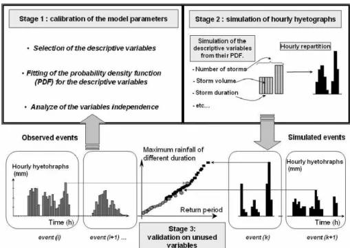
define the hourly rainfall signal into a rainfall event. Each variable was fitted by a prob-ability law (Cernesson et al., 1996). Monte Carlo methods were used to reproduce the rainfall signal from the generation of these variables. Then time series, statistically equivalent to observations, can be reproduced for any desired time period. Quantiles are empirically estimated from these simulated times series. The robustness and the

15

accuracy of these quantiles has been tested for the daily rainfall (Muller et al., 2009; Neppel et al., 2007). Figure 1 illustrates the generator’s principle.

2.2 Generator’s descriptive variables

First, the descriptive analysis of rainfall was based on rainfall events selected on daily criteria, i.e. a succession of daily rainfall depths of more than 4 mm, including one

20

(6)

HESSD

9, 11227–11266, 2012

Title Page

Tables Figures

◭ ◮

Back Close

Full Screen / Esc

Discussion

P

a

per

|

Dis

cussion

P

a

per

|

Discussion

P

a

per

|

Discussio

n

P

a

per

|

Based on these events, selected at daily intervals, the hourly rainfall signal is char-acterized by seven other descriptive variables. These variables are the number of rainy

periods within an event (NRP), the number of storms within a rainy period (NS), and

the dry duration that separates it from the next rainy periodDRP. The storm is the

ba-sic entity for the analysis of rainfall events, and is defined as a succession of hourly

5

rainfall accumulations with a single local maximum. Each storm is characterized by its

duration (DS) and its volume (VS). The quantitative analysis of storm volumes and

du-rations showed the need to distinguish two types of storm called “major” and “ordinary” storms, and therefore to create a storm typology based on a daily criterion (Fine and Lavabre, 2002). This storm typology enables us to extract the main information from

10

rainfall modelling (Arnaud et al., 2007). Furthermore, two other variables have been introduced to characterize the hourly rainfall itself: the ratio between the hourly peak of

the storm and its volume (1/DS≤RXS≤1) and the relative position of the maximum

(1≤RPX_S≤DS). These allow for a satisfactory representation of the different hourly

rainfall patterns. Figure 2 illustrated an example of a rainy event where the different

15

descriptive variables are presented.

2.3 Model calibration

A first study carried out by Cernesson et al. (1996) determined the most adapted prob-ability laws to the various descriptive variables. The objective of the model regional-ization (realized on the whole French territory) led us to define the same theoretical

20

law for a given variable, whatever the studied station. For example, an exponential law has been chosen for the storm volume, and Poisson’s law for the duration storm, whatever the studied station. Only parameters of these probability laws distinguish the

climate (Arnaud et al., 2007). Calibrating the generator consists in estimating different

parameters of the chosen probability laws with observed rainfall in a given rain gauge

25

station. 20 parameters are required to fully calibrate the rainfall generator for two dif-ferent seasons namely the “winter” season from December to May and the “summer”

(7)

HESSD

9, 11227–11266, 2012

Title Page

Tables Figures

◭ ◮

Back Close

Full Screen / Esc

Discussion

P

a

per

|

Dis

cussion

P

a

per

|

Discussion

P

a

per

|

Discussio

n

P

a

per

the precipitation regimes. Note that some of the 20 parameters either vary only slightly or have very little impact on the results.

2.4 Simulation and rainfall quantiles estimation

After the model calibration, in order to simulate a rainy event, all descriptive variables are generated in a specific order. Many rainy events are created to build time series

5

as long as wanted in which the average number of observed events per year for each

season are respected. To reduce the sampling effect on the simulated events, we chose

to generate rainfall on periods which were a thousand times longer than the strongest return period which we want to determine. For example, a 100 yr-quantile is determined by generated hyetographs on a 100 000 yr simulation period. Quantiles can then be

10

empirically estimated from these simulated times series without uncertainty due to the sampling variability.

At the beginning, the descriptive variables of the model were considered statistically independent. Many studies highlighted that some variables are dependent according to observations and that the dependence modelization is needed in order to reproduce

15

the rainfall signal. Indeed, Arnaud et al. (2007) shows that the model can reproduce extreme rainfall for all types of climate by adding a dependence structure between the depths of successive rainstorms. In this paper, we focus on the dependence between two variables: the depth and the duration of a rainstorm.

2.5 An operational model

20

Prima facie, SHYPRE appears to be a complex model due to the number of variables or

the di_fferent typologies used to define them. Nevertheless, an e_ffort has been made to

simplify it enabling an application on many hydrological problems. For example, Cantet et al. (2011) detected climate change impact on extreme rainfall throughout the model parameters; the SHYPRE outputs are also used to determine the dimension of a dam

(8)

HESSD

9, 11227–11266, 2012

Title Page

Tables Figures

◭ ◮

Back Close

Full Screen / Esc

Discussion

P

a

per

|

Dis

cussion

P

a

per

|

Discussion

P

a

per

|

Discussio

n

P

a

per

|

with a radar (Fouchier, 2007) or in a flash flood warning (Javelle et al., 2010). A

region-alized version of the model allows the estimation of rainfall quantiles for di_fferent time

durations on a square of 1 km2everywhere in the French territory (Arnaud et al., 2006).

3 How to diagnose and model the dependence

The aim of this part is to introduce the mathematical tools used in the study of

depen-5

dence between random variables. Only tools used in our study are clearly presented. For further information, see Nelsen (2006) and Genest and Favre (2007).

3.1 Measuring dependence: Kendall’s tau

Classically, dependence is measured by correlation coefficients. The most well-known

is Pearson’s coefficient (R) used for example in a linear regression. It only

character-10

izes a linear dependence between two variables. When the dependence is not linear, a correlation computed on ranks appears to be the best approach (Oakes, 1982)

lead-ing to the buildlead-ing of two other correlation coefficients: Spearman’s rho and Kendall’s

tau. Only Kendall’s tau (notedτ) is presented in this paper:

Suppose that a random sample (X1,Y1),. . ., (Xn,Yn) is given from some pair (X,Y)

15

of continuous variables. Here,R_i stands for the rank of X_i among X1,. . .,Xn, and Si

stands for the rank of Y_i among Y₁,. . .,Y_n. The empirical version of Kendall’s tau is

given by:

τ_n = Pn−Qn

n(n−1)/2 = 4

n(n−1)Pn−1 (1)

where P_n and Q_n are the number of concordant and discordant pairs, respectively.

20

Here, two pairs (Xi,Yi), (Xj,Yj) are said to be concordant when (Xi−Xj)(Yi−Yj)>0,

and discordant when (X_i−X_j)(Y_i−Y_j)<0. The borderline case (X_i−X_j)(Y_i−Y_j)=0

occurs with a probability zero under assumption that X and Y are continuous. The

(9)

HESSD

9, 11227–11266, 2012

Title Page

Tables Figures

◭ ◮

Back Close

Full Screen / Esc

Discussion

P

a

per

|

Dis

cussion

P

a

per

|

Discussion

P

a

per

|

Discussio

n

P

a

per

It is obvious that τ_n is a function of the ranks of the observations only, since (X_i−

Xj)(Yi−Yj)>0 if and only if (Ri−Rj)(Si−Sj)>0.

If X and Y are mutually independent, we have τ_n≈0. The closer to 1|τ_n| is, the

stronger the dependence between two variables. Ifτ_n>0 (resp.<0), the dependence

is positive (resp. negative).

5

An independence test can be based onτ_n, since underH0: independence between

two variables,big this statistic is close to normal with zero mean and variance 2(2n+

5)/(9n(n+1)). For example, we can reject H0 with a significance level (type I error)

α=5 % ifq₂₍₂9n(_nn₊+1)₅₎|τ_n| > z_α/2 =1.96.

With discrete variables, this statistical test is biased by the ties. An unbiasing test

10

consists in replacingnbyn−number of ties in the variance calculus under H0.

How-ever, this case will be discussed further.

3.2 Modelling dependence: copula approach

Traditionally, the pairwise dependence between variables has been described using classical families of multivariate distributions. The main limitation of this approach is

15

that the individual behavior of the two variables must be characterized by the same

parametric family of univariate distributions. The copula model, introduced by (Hoeff

d-ing, 1940; Sklar, 1959), is more and more widespread since it avoids this restriction. For simplicity purposes, we restrict attention to the bivariate case in this paper. A bidimensional copula, also called a 2-copula, is a two-place real function defined

20

on [0, 1]×[0, 1]→ [0, 1] such as

1. ∀u,v ∈[0, 1],

C(u, 0)=0,C(u, 1)=u,C(0,v)=0,C(1,v)=v;

2. ∀u1,u2,v1,v2 ∈[0, 1] such asu1≤u2andv1≤v2,

C(u2,v2)−C(u2,v1)−C(u1,v2)+C(u1,v1)≥0

(10)

HESSD

9, 11227–11266, 2012

Title Page

Tables Figures

◭ ◮

Back Close

Full Screen / Esc

Discussion

P

a

per

|

Dis

cussion

P

a

per

|

Discussion

P

a

per

|

Discussio

n

P

a

per

|

F_{X Y} a joint cumulative distribution function of any pair of (X,Y) of continuous random

variables can be written in the form

FX Y(x,y) =C(FX(x),FY(y)) , ∀x,y ∈R (2)

whereF_X and F_Y are the marginal functions andC: [0, 1]×[0, 1]→[0, 1] is a copula.

Sklar (1959) showed thatC,F_X, andF_Y are uniquely determined whenF_{X Y} is known,

5

a valid model for (X,Y) arises from Eq. (2) whenever the three “ingredients” are chosen

from given parametric families of distributions.

The main advantage of the copula approach is that the choice of the dependence

model betweenX andY does not depend on the marginal distributions.

For a random sample (X1,Y1),. . ., (Xn,Yn) from some pair (X,Y), anempirical copula

10

can be introduced, and is defined by

Cn(u,v)=

1

n

X

i=1 1₍_F

X(Xi)≤u∩FY(Yi)≤v) (3)

where1(.)denotes the indicator function,FX andFY are the marginal distributions ofX

andY.

3.3 Estimation and choice of models

15

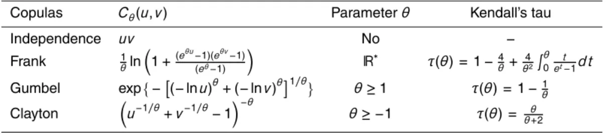
Modeling dependence between two random variables (X and Y) can be achieved by

using some families of copulas. In this paper, we only considered 3 archimedean copu-las: the Frank copula (Frank, 1979), the Clayton copula (Clayton, 1978), and the Gum-bel copula (GumGum-bel, 1961). These copulas have been chosen because they have only one parameter and are easily applicable.

20

Like usual statistic laws, different methods are used to estimate copula parameters.

(11)

HESSD

9, 11227–11266, 2012

Title Page

Tables Figures

◭ ◮

Back Close

Full Screen / Esc

Discussion

P

a

per

|

Dis

cussion

P

a

per

|

Discussion

P

a

per

|

Discussio

n

P

a

per

(Genest et al., 1995). For other methods, see Joe (1997), Tsukahara (2005) and Gen-est et al. (2008a). In this study, we Gen-estimated the copula parameter with the Kendall’s tau.

In typical modelling exercises, the user can choose between many different

depen-dence structures. Consequently, a method is necessary to select, among different

cop-5

ulas, the best adapted dependence structure for the studied data. For the unidimen-sional law, several tests provide the best fitting to the observations, for example the Kolmogorov-Smirnov test. To test the suitability of copula models, the same principle can be used. For example, we can compare the empirical copula (defined in Eq. (3)) to a theoretical copula through the calculation of the Kolmogorov-Smirnov statistic or

10

through a QQ-plot. In this way, Genest and Rivest (1993); Hillali (2001) proposed a test for the Archimedean copulas. Genest et al. (2008b) compared a lot of measures to choose the best copula. Genest and R ´emillard (2008) use a bootstrap procedure for suitability testing. This test has been implemented in the “copula” package (Yan, 2007) from the language R (http://www.r-project.org/).

15

3.4 Generating a pair from a copula

Simple simulation algorithms are available for most copula models, e.g. Devroye (1986, Ch. 2), or Whelan (2004) for the Archimedean copulas. In the bivariate case, a good

strategy for generating a pair (U,V) from a copulaC consists in using the conditional

distributions:

20

1. Generateufrom a uniform distribution on the interval [0, 1],

2. GivenU=u, generate from the conditional distribution:

Q_u(v) =P V ≤v|U =u= _∂u∂ C(u,v)

(12)

HESSD

9, 11227–11266, 2012

Title Page

Tables Figures

◭ ◮

Back Close

Full Screen / Esc

Discussion

P

a

per

|

Dis

cussion

P

a

per

|

Discussion

P

a

per

|

Discussio

n

P

a

per

|

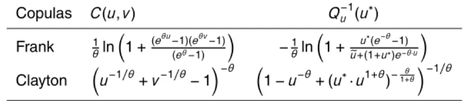
The explicit formulas forQ−_u1are illustrated in the Table 2 for the Frank and Clayton

copulas. For the Gumbel copula, no explicit formula exists, the valuev =Q−_u1(u◦) can

be determined by a numerical approach2.

To avoid using an optimization algorithm, Embrechts et al. (2003) or Mc Neil (2008)

propose to generate directly the pair (U,V). In our case, the latter approach is not

5

suitable since the storm duration must be generated for a given volume storm (already generated Arnaud et al., 2007).

3.5 The discrete variable case

In the context of dependence, the methods described above depend on the continu-ity assumptions for the marginal distributions. In the case of discrete variables, many

10

desirable properties of dependence measures no longer hold. The main technical ar-gument consists in a continuous extension of integer-valued random variables. Here, we used the method proposed by (Denuit and Lambert, 2005).

Assume thatX is a discrete variable and X ≥0. We associateX with a continuous

randomX∗such as

15

X∗ =X +(U−1), whereU ∼ U[0, 1]. (4)

4 Application into the rainfall generator: Depth/Duration dependence

The subject of this section is to apply the copula approach to the rainfall generator to simulate the relationship between the depth and duration of a rainstorm. This

relation-ship is called further theDepth/Duration dependence. Only major storms are taken into

20

account to study this dependence.

2

(13)

HESSD

9, 11227–11266, 2012

Title Page

Tables Figures

◭ ◮

Back Close

Full Screen / Esc

Discussion

P

a

per

|

Dis

cussion

P

a

per

|

Discussion

P

a

per

|

Discussio

n

P

a

per

First, the data used in the study are briefly presented. Then, the mathematical tools, presented in Sect. 3, are applied to model this dependence. Finally, the impacts on the rainfall quantiles estimation are illustrated.

4.1 Presentation of data used

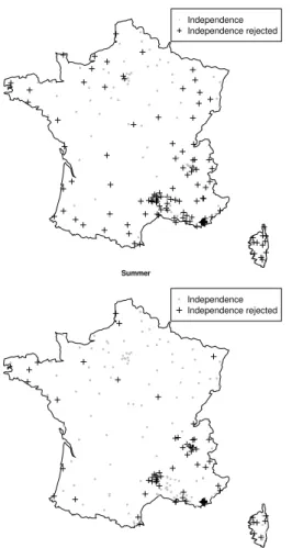
217 rain-gauge stations are used in metropolitan France (Fig. 3). Among the 217

sta-5

tions studied, 173 are reference rainfall stations for the French weather office M ´et

´eo-France (synoptic network). The others are stations with long observation records, and data that have been validated by management agencies – mainly Cemagref; DDE,

the local o_ffices of the France Ministry of Equipment; and Diren, the regional

environ-ment authorities. If all stations are taken into account, the median observation period

10

is 17.8 yr, with observation periods ranging from a few years for some of the alpine sta-tions to 78 yr for the rainfall series in Marseille. The sampling of data used in this study indicates an extremely wide range of rainfall values, providing the opportunity to see how the hourly rainfall models perform in highly diverse contexts. Arnaud et al. (2007) used the same stations and presented them in further details.

15

4.2 TheDepth/Duration dependence model

In the rainfall generator, the volume of a rainstorm, noted V, follows an exponential

law while the duration of a rainstorm, notedD, follows a Poisson’s law, a discrete law.

Consequently, the method described in Sect. 3.5 is applied to transformDtoD∗without

losing information.

20

4.2.1 Where is theDepth/Duration dependencesignificant?

First Kendall’s tau between V and D∗ is estimated on each of the 217 rain gauge

(14)

HESSD

9, 11227–11266, 2012

Title Page

Tables Figures

◭ ◮

Back Close

Full Screen / Esc

Discussion

P

a

per

|

Dis

cussion

P

a

per

|

Discussion

P

a

per

|

Discussio

n

P

a

per

|

determine, from the 217 obtained p-values3, the number of rejected null hypothesis,

that is the number of stations for which theDepth/Durationindependence hypothesis

is rejected at a fixed significance levelα=0.05 (type I error).

The null hypothesisH0: independence betweenV and D∗ is not rejected for all

sta-tions. Actually the significance of the dependence seems to depend on the season and

5

the geographical location (climate) (See Fig. 3). In Winter, 140 among 217 rain gauge stations have a significant positive dependence, that is to say, a storm with a big volume is usually associated with a storm with a long duration (on these 140 stations). In Sum-mer, only 81 stations have a significant positive dependence, these stations are mostly located in the mountain landscape or near the ocean. These results are

climatologi-10

cally consistent. Indeed, summer rainfall, especially in the continental climate, occur in rainy phenomena providing rainstorms with a strong intensity and a short duration (convective systems).

4.2.2 How can theDepth/Duration dependencebe modelled?

The goal is to maintain a single model structure: only model parameters can distinguish

15

the climate. Therefore only one copula should be used to model theDepth/Duration

dependencefor any station.

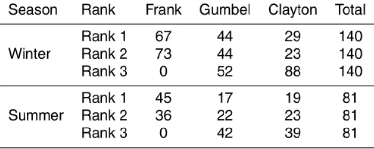
On each station where the dependence is significant (140 for Winter and 81 for

Summer), theL2-distance between the empirical copula and the 3 theoretical copulas

is calculated and is ordered. The best copula, that is to say the copula whose distance

20

is minimum, has the rank 1. Most of the time, the copula which is selected is the Frank copula (see Table 3). When another copula seems to be better (it often occurs when the numbers of storms is lower than 40), the Frank copula is always the second

best copula, never the “worst” copula. Besides, the L2-distance for the Frank copula

3

the p-value is the probability of obtaining a result at least as large as the one actually observed, given that the null hypothesis is true. In our case, it corresponds toP(X >tau) where

(15)

HESSD

9, 11227–11266, 2012

Title Page

Tables Figures

◭ ◮

Back Close

Full Screen / Esc

Discussion

P

a

per

|

Dis

cussion

P

a

per

|

Discussion

P

a

per

|

Discussio

n

P

a

per

is close to theL2-distance for the best copula. Finally, there is no specific geographic

localization where the Frank copula is not the best one.

This procedure is not a formal test, it only permits to define the best adapted copula among others according to a criterion. To assure the goodness-of-fit, the test presented

by (Genest and R ´emillard, 2008)4has been performed on each station where the

de-5

pendence is significant. As for the independence test, the FDR procedure is applied on

thep-values (140 for Winter and 81 for Summer). No null hypothesis – Frank copula is

well adapted – is rejected at a fixed significance levelα=0.05 for Winter and Summer.

Note that, the same test has been performed for the Gumbel copula and only 5 (resp. 2) null hypothesis are rejected for Winter (resp. Summer). For the Clayton copula, 102

10

(resp. 69) null hypothesis are rejected for Winter (resp. Summer).

The Frank copula is chosen to model the Depth/Duration dependence for any station.

The parameterθof the copula is estimated with the inversion of Kendall’s tau which is

estimated on each station (as shown in Fig. 3). Therefore, the shifting from one climate

to another is possible based uniquely on the parameterθ.

15

4.3 Impacts on the rainfall quantiles estimated by the generator

The Depth/Duration dependence modelling (by Frank and Gumbel copulas) has been implemented into the rainfall generator as shown in the Sect. 3.4. Simulations were performed on all 217 available stations and the performance of the new model was compared to the performance of the model that does not take into account the

20

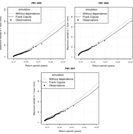
Depth/Duration dependence for all stations. The model is only tested in terms of repro-duction of the maximum rainfall of an event. Testing autocorrelation, cross-validation or intermittency is not the subject of the paper.

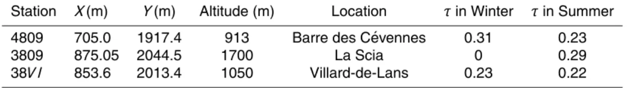
First, the impact of the Depth/Duration dependence modelling is illustrated by the plotting of the frequency distributions for 1-h maximum rainfall for three stations (see

25

(16)

HESSD

9, 11227–11266, 2012

Title Page

Tables Figures

◭ ◮

Back Close

Full Screen / Esc

Discussion

P

a

per

|

Dis

cussion

P

a

per

|

Discussion

P

a

per

|

Discussio

n

P

a

per

|

the positive dependence is significant. Nevertheless the new model allows a better es-timation according to the observations. Indeed, without the dependence modelling, the generator seems to overestimate 1-h rainfall. Note that, the quantiles with the Gumbel copula model are not shown in Fig. 4 because they are very close to Frank’s quantiles.

Then, we also compared the quantiles obtained from fitting an exponential law5 to

5

the observation samples (notedQT_obs) with quantiles from simulations of rainfall events

(notedQT_RG) according to two criteria:

1. The relative error given by

Error =100Q

T

RG−Q

T

obs

QT_obs (5)

is calculated on each 217 available stations. Its distribution is illustrated by a

box-10

plot where whiskers corresponding to the 0.05 and 0.95 quantile (See Fig. 5).

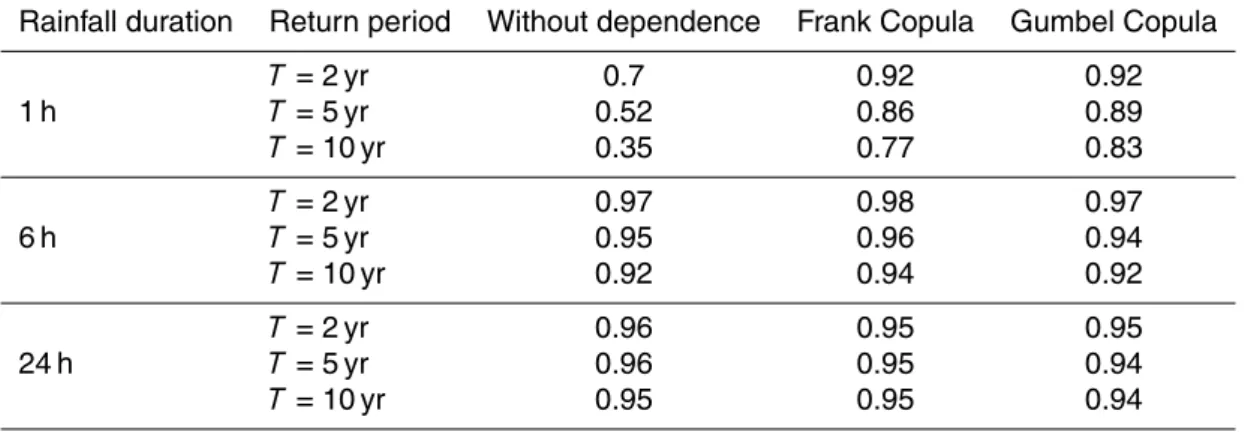
2. The Nash criterion (Nash and Sutcliffe, 1970) given by

Nash =1−

n

X

i=1

(QT_obs−QT_RG)2

n

X

i=1

(Q_obsT −QT_obs)2

(6)

whereQT_obs=n1

n

X

i=1

QT_obs andnis the number of studied stations. It is widely

con-sidered that Nash≥0.7 signifies that the two series are similar. Table 5 illustrated

15

5

(17)

HESSD

9, 11227–11266, 2012

Title Page

Tables Figures

◭ ◮

Back Close

Full Screen / Esc

Discussion

P

a

per

|

Dis

cussion

P

a

per

|

Discussion

P

a

per

|

Discussio

n

P

a

per

the value of the Nash criterion forT =2, 5, 10 yr calculated on the 217 available

stations coming from quantiles estimated by the two models.

Rainfall patterns can be distinguished according to the ratio between the short

dura-tion rainfall and long duradura-tion rainfall. Figure 6 illustrated the difference (like in Eq. (5))

betweenR_obsT andR_RGT where:

5

R_obsT (D1,D2)=Q

T

obs(D1)

QT_obs(D2) and R

T

RG(D1,D2)=

QT_RG(D1)

QT_RG(D2) (7)

D1 orD2 being the duration of the maximum rainfall with D1=1 h or 6 h andD2=6 h

or 24 h.

Results presented in Table 5 and Figs. 5 and 6 show an obvious gain of the copula used to reproduce hourly extreme rainfall. Indeed quantiles are globally more similar

10

to observed data when dependence is modelled for both models (Gumbel or Frank). This improvement is due to a better grasp of the observed phenomena. Modelling the Depth/Duration dependence results in a more accurate plotting of rainfall quantiles,

especially for the sub-daily maximum rainfall, enables us to generate different rainfall

patterns. The copula choice in the Depth/Duration dependence modelling leads to little

15

impact on the estimation of rainfallT-quantiles withT ≤10 yr for any duration.

The previous part showed that quantiles estimated by the new models are similar to

the quantiles coming from a fitting by an exponential forT ≤10 yr. Dealing with (very)

extreme values, finding a relevant accuracy test is not an easy task6.

Arnaud et al. (2008) proposed a simple test which is also used in (Garavaglia et al.,

20

(18)

HESSD

9, 11227–11266, 2012

Title Page

Tables Figures

◭ ◮

Back Close

Full Screen / Esc

Discussion

P

a

per

|

Dis

cussion

P

a

per

|

Discussion

P

a

per

|

Discussio

n

P

a

per

|

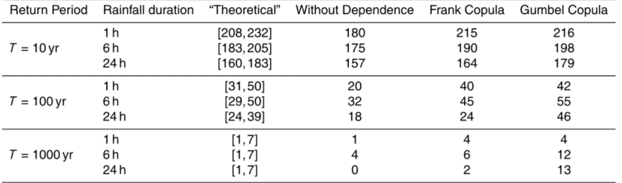
performed on 414 rain gauge stations7. Table 6 shows the number of stations where

theT-quantiles are exceeded by the maximum observed rainfall.

The results of the accuracy test show that the model without dependence proposes overestimated extreme quantiles, especially for the sub-daily rainfalls. Unlike the mod-els where the Depth/Duration dependence is modeled, the number of stations where

5

the observed records exceed extreme quantiles is too small compared to the “theoret-ical” number. Modelling dependence allows the researchers to obtain extreme rainfall quantiles that are coherent with the accuracy test for the sub-daily rainfall. The choice

of the copula (Frank versus Gumbel) affects the rainfall quantiles for durationD >1 h,

especially when the return period is high. Unlike the Frank copula, the Gumbel

cop-10

ula “amplifies” the dependence in extreme values leading to a clear underestimation for daily rainfall extreme quantiles. An extreme rainfall event is often constructed from a succession of heavy storms (persistence phenomenon in Arnaud et al., 2007). Gen-erating too long durations for these heavy storms causes a decrease of the number of rainstorms occurring in 24 h leading to a decrease of daily rainfall depth.

15

5 Discussion and conclusions

In this paper, the copula approach is applied into a stochastic hourly rainfall generation model. With this tool, any dependence can easily be taken into account in an existing stochastic model, because a copula process permits the desciption of the dependen-cies between many random variables, independently of their marginal distributions. It

20

has been applied to generate a relation between the depth and the duration of a rain-storm.

The rainfall generator has been developed to be applicable for all types of climate. The rainfall model structure is the same for any station, a shifting from one climate to

7

(19)

HESSD

9, 11227–11266, 2012

Title Page

Tables Figures

◭ ◮

Back Close

Full Screen / Esc

Discussion

P

a

per

|

Dis

cussion

P

a

per

|

Discussion

P

a

per

|

Discussio

n

P

a

per

another is possible based uniquely on the model’s parameters. To continue in the same way, only one copula has been chosen to model the same structure of dependence on any sites. A procedure has been performed to find the best adapted copula among others. For both seasons, the Frank copula appears to be the best for most of the sites, according to our criteria, and has been validated by a formal goodness-of-fit test.

5

No influence seems to be exerted by the rain gauge locations over the dependence structure. Here, two seasons are distinguished into the generator calibration. A future

version of the model will distinguish different weather patterns based on meteorological

circulation used in Garavaglia et al. (2010). This distinction could lead to use different

copulas for each class of weather providing a better generation of all rainfall patterns.

10

Taking dependence into account enables the researchers to improve the results of the rainfall model, especially in the sub-daily rainfall generation. The copula choice in the Depth/Duration dependence modelling (Gumbel or Frank) leads to minor impact

on the estimation of rainfallT-quantiles withT ≤10 yr for any duration. The two criteria

used have shown that the proposed model could reproduce the standard statistics of

15

maximum rainfall for all durations. Indeed biennial or decennial quantiles estimated by the model are close to those estimated by a fitting on observations: the relative errors

are centred to 0 and do not exceed±20 % for 95 % of 217 available stations. Stations

can be clustered according to three different types of climate: alpine, temperate and

Mediterranean to test the model’s performance in each type of climate. For the three

20

climates, the Frank copula seems to be the best adapted and the two criteria (relative error and the Nash criterium) are approximately the same for each type of climate. However, simulated hourly rainfall in the alpine climate seems to be overestimated in the high elevation site. This overestimation can be caused by the fact that the snow can lead to inaccurate knowledge of the real rainfall intensity.

25

(20)

HESSD

9, 11227–11266, 2012

Title Page

Tables Figures

◭ ◮

Back Close

Full Screen / Esc

Discussion

P

a

per

|

Dis

cussion

P

a

per

|

Discussion

P

a

per

|

Discussio

n

P

a

per

|

heaviest storms leading an underestimation on the daily rainfall quantiles. As previously mentioned, this test should be performed in each climate but the authors think the number of stations is too small to apply it. However, the location of the stations where the quantiles have been exceeded can give an idea of the good representation of all types of climate. For example, the stations where the decennial quantile is exceeded

5

are well distributed all over France. It is similarly for the centennial quantiles except for alpine sites where no centennial quantiles are exceeded. It can be explained by the relatively short observation periods (about 10 yr for the alpine stations).

To conclude, the proposed model can reproduce the standard and extreme statistics of maximum rainfall for any duration. Only one parameter has been added compared

10

to the previous version. It has been regionalized and can provide rainfall quantiles on ungauged sites (Arnaud et al., 2006). The additional parameter can be explained by geographical variables and has been regionalized to apply the proposed version of the rainfall generator in the whole France leading to an improvement of the estimation of the hourly rainfall quantiles.

15

Note that, in this study, copulas are applied to model the Depth/Duration dependence but their application can be extended to many dependencies. In another study, the “per-sistence” phenomenon (dependence between the depth of rainstorms in a rainy event) introduced by (Arnaud et al., 2007), is modeled by an approach based on copulas, providing good results in extreme rainfall generation.

20

Appendix A

Controlling the global significance level of a multiple tests approach using the False Discovery Rate (FDR): the Benjamini and Hochberg (BH) procedure

Benjamini and Hochberg (1995) proposed a procedure to control the global

signifi-cance levelαgof a multiple tests procedure. Assuming thatK tests of a null hypothesis

25

(21)

HESSD

9, 11227–11266, 2012

Title Page

Tables Figures

◭ ◮

Back Close

Full Screen / Esc

Discussion

P

a

per

|

Dis

cussion

P

a

per

|

Discussion

P

a

per

|

Discussio

n

P

a

per

1. Letp(1)≤p(2) ≤. . .≤p(K)be the sorted observed p-values related to theK tests;

2. Computem=max{1 ≤j≤K,p(j) ≤

j K α};

3. If m exists, then reject among the K hypothesis the m ones corresponding to

p(1) ≤. . .≤p(m)p-values; else reject no hypothesis.

Appendix B

5

An accuracy test for the extreme values

A procedure has proposed to test the pertinence of extreme quantiles estimated by a method. This test can be performed on many stations.

Let be NYi the number of years of observation at the stationi.

Let be NEi the number of rainfall events observed during the NYi years at the

sta-10

tioni.

Let be NEidef= NE_NAii: the average number of events per year for the stationi.

Xi ={X_ji}_j₌1...NEi: the depth of the rainfall observed during the NE

i

rainy events.

X_Si =max{X_ji}_j₌₁_..._NEi: the maximum rainfall observed at the stationi.

q_Ti: the “true” quantile with the return periodT years at the stationi

15

c

q_Ti: the quantile with the return periodT years at the stationi estimated by the tested

method.

Nsup: the number of stations, amongN, whereq

i

T is exceeded byX

i

S.

d

nsup: the number of stations, amongN, whereqcTi is exceeded byX

i

S.

The goal is to define the theoretical law ofNsup.

(22)

HESSD

9, 11227–11266, 2012

Title Page

Tables Figures

◭ ◮

Back Close

Full Screen / Esc

Discussion

P

a

per

|

Dis

cussion

P

a

per

|

Discussion

P

a

per

|

Discussio

n

P

a

per

|

Assuming that theX_j are independent, we have:

P(X_Si < x) =

NEi

Y

j=1

P(X_ji < x)

=P(X_ji < x)NE

i

5

By definition, P(X_ji < q_Ti)=1− 1

T×NEi

. Therefore, we obtain P(X_Si > q_Ti) =1−1−

1

T×NEi

NEi

On each station, a Bernouilli draw is realized where the success

probabil-ity P(X_Si > qi_T) depends on NEi and NEi. Consequently, this success probability is

different from a station to another:Nsup does not follow an usual binomial distribution.

The idea is to approach this distribution by a Monte-Carlo method.

10

When the observed records are considered independent between them, the following

procedure is proposed to approximate the theoretical distribution ofNsup:

Let beNsima large number

fork=1 :Nsim do

Nsupk =0

15

fori =1 :N do

u∼ U[0, 1]

ifu <1−1− 1

T×NEi

NEi

thenNsupk =Nsupk +1

end for end for

20

Nsim values of the random variable Nsup have been performed to obtain Πe(x) an

approximation ofΠ(x), the theoretical distribution ofNsup. Then, it is easy to estimate

(23)

HESSD

9, 11227–11266, 2012

Title Page

Tables Figures

◭ ◮

Back Close

Full Screen / Esc

Discussion

P

a

per

|

Dis

cussion

P

a

per

|

Discussion

P

a

per

|

Discussio

n

P

a

per

construction of a confidence intervalIconfofNsup has been chosen. Ifndsup ∈ Iconfthen

the quantileqc_Ti estimated by the method appears to be correct according to the data. If

d

nsupis too large (respectively small), the method seems to underestimate (respectively

overestimate) rainfall quantiles.

To obtain the independence between the observed records (a strong hypothesis to

5

constructΠe(x)), we propose to delete the stations where their records occur on the

same day (only one station is kept, randomly chosen). Thus, the confidence interval

Iconfcan differ according to the rainfall duration.

References

Adams, B. and Papa, F.: Urban Stormwater Management Planning with Analytical Probabilistic

10

Models, John Wiley & Sons, New York, 2000. 11229

Arnaud, P.: Mod èle de pr édetermination de crues bas é sur la simulation stochastique des pluies horaires, Ph.D. thesis, Universit é Montpellier II, Montpellier, 1997. 11231

Arnaud, P. and Lavabre, J.: Using a stochastic model for generating hourly hyetographs to study extreme rainfalls, Hydrolog. Sci. J., 44, 433–446, 1999. 11230

15

Arnaud, P. and Lavabre, J.: Coupled rainfall model and discharge model for flood frequency estimation., Water Resour. Res., 38, 1075–1085, 2002. 11230

Arnaud, P. and Lavabre, J.: Estimation de l’al ´ea pluvial en France m ´etropolitaine, Editions QUAE, Versailles, 2010. 11231

Arnaud, P., Lavabre, J., Sol, B., and Desouches, C.: Cartographie de l’al ´ea pluviographique de

20

la France, La Houille Blanche, 5, 102–111, 2006. 11230, 11234, 11246

Arnaud, P., Fine, J., and Lavabre, J.: An hourly rainfall generation model adapted to all types of climate., Atmos. Res., 85, 230–242, 2007. 11230, 11231, 11232, 11233, 11238, 11239, 11244, 11246, 11261

Arnaud, P., Lavabre, J., Sol, B., and Desouches, C.: R égionalisation d’un g én érateur

25

(24)

HESSD

9, 11227–11266, 2012

Title Page

Tables Figures

◭ ◮

Back Close

Full Screen / Esc

Discussion

P

a

per

|

Dis

cussion

P

a

per

|

Discussion

P

a

per

|

Discussio

n

P

a

per

|

Bacchi, B., Becciu, G., and Kottegoda, N.: Bivariate exponential model applied to intensities and durations of extreme rainfall, J. Hydrol., 155, 225–236, doi:10.1016/0022-1694(94)90166-X, 1994. 11229

Balistrocchi, M. and Bacchi, B.: Modelling the statistical dependence of rainfall event variables through copula functions, Hydrol. Earth Syst. Sci., 15, 1959–1977,

doi:10.5194/hess-15-5

1959-2011, 2011. 11230

B ´ardossy, A. and Pegram, G. G. S.: Copula based multisite model for daily precipitation simula-tion, Hydrol. Earth Syst. Sci., 13, 2299-2314, doi:10.5194/hess-13-2299-2009, 2009. 11229 Benjamini, Y. and Hochberg, Y.: Controlling the false discovery rate: a practical and powerful

approach to multiple testing, J. Roy. Stat. Soc. B Met., 57, 289–300, 1995. 11246

10

Cantet, P., Bacro, J., and Arnaud, P.: Using a rainfall stochastic generator to detect trends in extreme rainfall, Stoch. Env. Res. Risk A., 25, 429–441, 2011. 11233

Carvajal, C., Peyras, L., and Arnaud, P., Boissier, D., and Royet, P.: Probabilistic Modeling of Floodwater Level for Dam Reservoirs, J. Hydrol. Eng., 14, 223–232, 2009. 11233

Cernesson, F.: Mod èle simple de pr édetermination des crues de fr équences courantes à rares

15

sur petits bassins versants m édit éran éens., Ph.D. thesis, Universit é Montpellier II, Montpel-lier, 1993. 11231

Cernesson, F., Lavabre, J., and Masson, J.: Stochastic model for generating hourly hyetograph, Atmos. Res., 42, 149–161, 1996. 11230, 11231, 11232

Clayton, D.: A model for association in bivariate life tables and its application in epidemiological

20

studies of familial tendency in chronic disease incidence, Biometrika, 65, 141–151, 1978. 11236

C ´ordova, J. R. and Rodr´ıguez-Iturbe, I.: On the probabilistic structure of storm surface runoff, Water Resour. Res, 21, 755–763, doi:10.1029/WR021i005p00755, 1985. 11228

De Michele, C. and Salvadori, G.: A Generalized Pareto intensity-duration model of storm

rain-25

fall exploiting 2-Copulas, J. Geophys. Res., 108, 4067, doi:10.1029/2002JD002534, 2003. 11229

De Michele, C., Salvadori, G., Canossi, M., Petaccia, A., and Rosso, R.: Bivariate statistical approach to spillway design flood, J. Hydraul. Eng. ASCE, 10, 50–57, 2005. 11229

Denuit, M. and Lambert, P.: Constraints on concordance measures in bivariate discrete data,

30

J. Multivariate Anal., 93, 40–57, 2005. 11238

(25)

HESSD

9, 11227–11266, 2012

Title Page

Tables Figures

◭ ◮

Back Close

Full Screen / Esc

Discussion

P

a

per

|

Dis

cussion

P

a

per

|

Discussion

P

a

per

|

Discussio

n

P

a

per

D´_ıaz-Granados, M. A., Valdes, J. B., and Bras, R. L.: A physically based flood frequency distri-bution, Water Resour. Res., 20, 995–1002, doi:10.1029/WR020i007p00995, 1984. 11228 Eagleson, P.: Dynamics of flood frequency, Water Resour. Res., 8, 878–898, 1972. 11228 Eagleson, P.: Climate, soil, and vegetation. 2. The distribution of annual precipitation derived

from observed storm sequences, Water Resour. Res., 14, 713–721, 1978a. 11228

5

Eagleson, P.: Climate, soil, and vegetation. 5. A derived distribution of storm surface runoff, Water Resour. Res., 14, 741–748, 1978b. 11228

Eagleson, P.: Climate, soil, and vegetation. 7. A derived distribution of annual water yield, Water Resour. Res., 14, 765–776, 1978c. 11228

Embrechts, P., Lindskog, F., and Mcneil, A.: Modelling dependence with copulas and

applica-10

tions to risk management, Handbook of Heavy Tail Distributions in Finance, North Holland, Amsterdam, 324–384, 2003. 11238

Favre, A., El Adlouni, S., Perreault, L., Thiemonge, N., and Bobee, B.: Multivariate hydrological frequency analysis using copulas, Water Resour. Res., 40, W01101, 12PP, 2004. 11229 Fine, J. and Lavabre, J.: Synth èse des d ébits de crue sur l’Ile de la R éunion. Phase I : la

15

pluviom étrie. Él éments de r égionalisation du g én érateur de pluie., Tech. rep., Cemagref, Aix en Provence, 2002. 11232

Fouchier, C.: AIGA: an operational tool for flood warning in Southern France. Principle and performances on Mediterranean flash floods, In: Geophysical Research Abstracts of EGU, Vienne, 15–20 avril 2007, vol. 9, p. 02843, Copernicus, Gottingen, 2007. 11234

20

Frank, M.: On the simultaneous associativity of F(x,y) and x+y−F(x,y), Aeq. Math., 19, 194–226, 1979. 11236

Garavaglia, F., Gailhard, J., Paquet, E., Lang, M., Garc¸on, R., and Bernardara, P.: Introducing a rainfall compound distribution model based on weather patterns sub-sampling, Hydrol. Earth Syst. Sci., 14, 951-964, doi:10.5194/hess-14-951-2010, 2010. 11243, 11245

25

Gargouri-Ellouze, E. and Chebchoub, A.: Modelisation de la structure de dependance hauteur-duree d’evenements pluvieux par la copule de Gumbel/Modelling the dependence structure of rainfall depth and duration by Gumbel’s copula, Hydrolog. Sci. J., 53, 802–817, 2008. 11229

Genest, C. and Favre, A.: Everything you always wanted to know about copula

mod-30

(26)

HESSD

9, 11227–11266, 2012

Title Page

Tables Figures

◭ ◮

Back Close

Full Screen / Esc

Discussion

P

a

per

|

Dis

cussion

P

a

per

|

Discussion

P

a

per

|

Discussio

n

P

a

per

|

Genest, C. and R émillard, B.: Validity of the parametric bootstrap for goodness-of-fit testing in semiparametric models, Annales de l’Institut Henri Poincar é-Probabilit és et Statistiques, 44, 1096–1127, 2008. 11237, 11241

Genest, C. and Rivest, L.: Statistical inference procedures for bivariate Archimedean copulas, J. Am. Stat. Assoc., 88, 1034-1043, 1993. 11237

5

Genest, C., Ghoudi, K., and Rivest, L.: A semiparametric estimation procedure of dependence parameters in multivariate families of distributions, Biometrika, 82, 543–552, 1995. 11237 Genest, C., Masiello, E., and Tribouley, K.: Estimating copula densities through wavelets, Insur.

Math. Econ., 44, 170–181, 2008a. 11237

Genest, C., R ´emillard, B., and Beaudoin, D.: Goodness-of-fit tests for copulas: A review and a

10

power study, Insur. Math. Econ., 44, 199–213, 2008b. 11237

Ghosh, S.: Modelling bivariate rainfall distribution and generating bivariate correlated rainfall data in neighbouring meteorological subdivisions using copula, Hydrol. Process., 24, 3558– 3567, 2010. 11229

Goel, N. K., Kurothe, R. S., Mathur, B. S., and Vogel, R. M.: A derived flood frequency

distribu-15

tion for correlated rainfall intensity and duration, J. Hydrol., 228, 56–67, doi:10.1016/S0022-1694(00)00145-1, 2000. 11229

Gumbel, E.: Bivariate logistic distributions, J. Am. Stat. Assoc., 56, 335–349, 1961. 11236 Guo, Y. and Adams, B. J.: An analytical probabilistic approach to sizing flood control detention

facilities, Water Resour. Res, 35, 2457–2468, doi:10.1029/1999WR900125, 1999. 11228

20

Haberlandt, U., Ebner von Eschenbach, A.-D., and Buchwald, I.: A space-time hybrid hourly rainfall model for derived flood frequency analysis, Hydrol. Earth Syst. Sci., 12, 1353–1367, doi:10.5194/hess-12-1353-2008, 2008. 11229

Haberlandt, U., Hundecha, Y., Pahlow, M., and Schumann, A. H.: Rainfall Generators for Appli-cation in Flood Studies, Flood Risk Assessment and Management, edited by: Schumann, A.

25

H., Springer The Netherlands, 117–147, doi:10.1007/978-90-481-9917-4 7, 2011. 11229 Hillali, Y.: Test d’ajustement d’une loi bidimensionnelle; Application a des donnees

clima-tologiques, Rev. Stat. Appl., 49, 79–96, 2001. 11237

Hoeffding, W.: Maszstabinvariante Korrelationstheorie, Schrijtfenr. Math. Inst. Inst., Angew. Math. Univ. Berlin, 5, 179–233, 1940. 11229, 11235

30

(27)

HESSD

9, 11227–11266, 2012

Title Page

Tables Figures

◭ ◮

Back Close

Full Screen / Esc

Discussion

P

a

per

|

Dis

cussion

P

a

per

|

Discussion

P

a

per

|

Discussio

n

P

a

per

Joe, H.: Multivariate models and dependence concepts, Chapman & Hall/CRC, London, 1997. 11237

Kurothe, R. S., Goel, N. K., and Mathur, B. S.: Derived flood frequency distribution for negatively correlated rainfall intensity and duration, Water Resour. Res., 33, 2103–2107, 1997. 11229 Li, J. Y. and Adams, B. J.: Probabilistic models for analysis of urban runoff control systems,

5

J. Environ. Eng., 126, 3, 217–224, doi:10.1061/(ASCE)0733-9372(2000)126:3(217), 2000. 11228

McNeil, A.: Sampling nested Archimedean copulas, J. Stat. Comput. Sim., 78, 567–581, 2008. 11238

Muller, A., Arnaud, P., Lang, M., and Lavabre, J.: Uncertainties of extreme rainfall quantiles

10

estimated by a stochastic rainfall model and by a generalized Pareto distribution, Hydrolog. Sci., 54, 417–429, 2009. 11230, 11231

Nash, J. and Sutcli_ffe, J.: River flow forecasting through conceptual models part I – A discussion of principles, J. Hydrol., 10, 282–290, 1970. 11242

Nelsen, R.: An introduction to copulas, Springer Verlag, New York, 2006. 11229, 11234

15

Neppel, L., Arnaud, P., and Lavabre, J.: Connaissance r égionale des pluies extr êmes. Com-paraison de deux approches appliqu ées en milieu m édit éran éens, C. R. Geoscience, 339, 820–830, 2007. 11230, 11231

Oakes, D.: A model for association in bivariate survival data, J. Roy. Stat. Soc. B, 44, 414–422, 1982. 11234

20

Salvadori, G. and De Michele, C.: Frequency analysis via copulas: Theoretical as-pects and applications to hydrological events, Water Resour. Res., 40, W12511, doi:10.1029/2004WR003133, 2004. 11229

Salvadori, G. and De Michele, C.: Statistical characterization of temporal structure of storms, Adv. Water Resour., 29, 827–842, 2006. 11229

25

Salvadori, G., de Michele, C., Kottegoda, N., and Rosso, R.: Extremes in Nature: An Approach Using Copulas, Springer, Dordrecht, The Netherlands, 2007. 11229

Salvadori, G., De Michele, C., and Durante, F.: On the return period and design in a multivariate framework, Hydrol. Earth Syst. Sci., 15, 3293–3305, doi:10.5194/hess-15-3293-2011, 2011. 11229

30