An Approach to Finding Similarity Between Two Community Graphs Using Graph Mining Techniques

(1)

An Approach to Finding Similarity Between Two

Community Graphs Using Graph Mining Techniques

Bapuji Rao

PhD Scholar (CSE)

Biju Patnaik University of Technology (BPUT) Rourkela, Odisha, India

Saroja Nanda Mishra

CSE & A

Indira Gandhi Institute of Technology (IGIT) Sarang, Odisha, India

Abstract—Graph similarity has studied in the fields of shape retrieval, object recognition, face recognition and many more areas. Sometimes it is important to compare two community graphs for similarity which makes easier for mining the reliable knowledge from a large community graph. Once the similarity is done then, the necessary mining of knowledge can be extracted from only one community graph rather than both which leads saving of time. This paper proposes an algorithm for similarity check of two community graphs using graph mining techniques. Since a large community graph is difficult to visualize, so compression is essential. This proposed method seems to be easier and faster while checking for similarity between two community graphs since the comparison is between the two compressed community graphs rather than the actual large community graphs.

Keywords—community graph; compressed community graph; dissimilar edges; self-loop; similar edges; weighted adjacency matrix

I. INTRODUCTION

A graph arises in many situations like web graph of documents, a social network graph of friends, a road-map graph of cities. Graph mining has grown rapidly for the last two decades due to the number, and the size of graphs has been growing exponentially (with billions of nodes and edges), and from it, the authors want to extract much more complicated information. Graph similarity has numerous applications in social networks, image processing, biological networks, chemical compounds, and computer vision, and therefore it has suggested many algorithms and similarity measures. Graph similarity is that "a node in one graph is similar to a node in another graph if their neighborhoods are similar" [1].

II. LITERATURE SURVEY

Graphs are general object model; graph similarity has studied in many fields. Similarity measures for graphs have used in systems for shape retrieval [2], object recognition [3] or face recognition [4]. For all those measures, graph features specific to the graphs in the application, are exploited to define graph similarity. Examples of such features are given one to one mapping between the vertices of different graphs or the requirement that all graphs are of the same order.

A very common similarity measure for graphs is the edit distance. It uses the same principle as the well-known edit distance for strings [5, 6]. The idea is to determine the minimal number of insertions and deletions of vertices and edges to

make the compared graphs isomorphic. In [7], Sanfeliu and Fu extended this principle to attributed graphs, by introducing vertex relabeling as a third basic operation beside insertions and deletions. In [8], the measure is used for data mining in a graph.

The main idea behind the feature extraction method is that similar graphs probably share certain properties, such as degree distribution, diameter, and Eigen values [9]. After extracting these features, a similarity measure [10] is applied to assess the similarity between the aggregated statistics and, equivalently, the similarity between the graphs. In the iterative method "two nodes are similar if their neighborhoods are also similar".

In each iteration, the nodes exchange similarity scores, and this process ends when convergence has achieved. A successful algorithm belongs to this category is the similarity ﬂooding algorithm by Melnik et al. [11] applies in database schema matching. It solves the "matching" problem, and attempts to find the correspondence between the nodes of two given graphs. Another successful algorithm is SimRank [12], which measures the self-similarity of a graph, i.e., it assesses the similarities between all pairs of nodes in one graph. Furthermore, another successful recursive method related to graph similarity and matching is the algorithm proposed by Zager and Verghese [13]. This method introduces the idea of coupling the similarity scores of nodes and edges to compute the similarity between two graphs.

A new method to measure the similarity of attributed graphs proposed in [14]. This technique solves the problems mentioned in similarity measures for attributed graphs and is useful in the context of large databases of structured objects. First, BP-based algorithm implemented for graph similarity [1] uses the original BP algorithm as it is proposed by Yedidia [15]. This algorithm is naive and runs in O (n2) time.

III. PROPOSED METHOD

(2)

adopted the compression of large community graph to smaller one technique from [16].

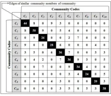
The authors have proposed a village community graph having ten communities namely C1 to C10, and the total number

of community members is 118. The black color edge represents the edge among the community members of similar communities. Whereas the blue color edge represents the edge among the community members of dissimilar communities.

Fig. 1. Community graph with communities {C1, C2, C3, C4, C5, C6, C7, C8, C9, C10}

Fig. 2. Compressed community graph of Fig.1

To compress the community graph to a smaller one depicted in "Fig. 1", the authors have adopted the logic from

[16]. The compressed community graph is depicted in “Fig. 2".

Then its corresponding adjacency matrix is represented in the memory and depicted in "Fig. 3". In this weighted adjacency matrix, the self-loop of the community has some weight and considered as a total number of edges among the community members of that particular community. Similarly, the edge between the pair of communities as the total number of edges between the community members of dissimilar communities. For this proposed approach, the authors have considered "Fig.

1" community graph as the principle community graph for comparison with six more community graphs namely CG2 to

CG7. Before comparison, these six community graphs, i.e.,

CG2 to CG7’s adjacency matrices are compressed and

represented in the memory. Finally, the principle community graph CG1’s compressed adjacency matrix has compared with

all the six community graphs, i.e., CG2 to CG7’s compressed

adjacency matrices for similarity check. The details of all the seven community graphs, CG1 to CG7 has considered as

datasets for the proposed algorithm is listed in "Table I".

Fig. 3. Adjacency matrix of Fig.2

IV. PROPOSED ALGORITHM

The proposed algorithm has three phases. Phase-1 is to open for reading four dataset files. The dataset files

commun1.txt and commun2.txt for reading number of communities, and community code and their total number of community members of two community graphs CG1 and CG2,

and assign to the matrices NCM1[][] and NCM2[][] respectively. Similarly two more dataset files data1.txt and

data2.txt for reading edge details of two community graphs CG1 and CG2, and assign to the matrices CMM1[][] and

CMM2[][] respectively. So Phase-1 is about read data and creation of community member matrices, and creation of initial form of compressed community matrices.

Pahse-2 for counting edges of community members of same communities by calling procedure SCED( ) and counting edges of community members of dissimilar communities by calling procedure DCED( ). Using procedures SCED( ) and DCED( ), the compressed community adjacency matrices CCM1[][] and CCM2[][] are assigned with the edge values and self loop values.

(3)

A. Algorithm for Community Graph Similarity

Algorithm Community_Graph_Similarity ( )

Algorithm Convention [17]

//CG1, CG2: Given two community graphs with 'n1' and 'n2'

//number of community members.

//tcm1, tcm2: To assign total community members of //community graphs CG1 and CG2.

//NCM1[n1][2], NCM2[n2][2]: Matrices to hold community //member’s community number and number of community //members of CG1 and CG2.

//CMM1[tcm1+1][tcm1+1], CMM2[tcm2+1][tcm2+1]:

//Adjacency matrices of CG1 and CG2.

//CCM1[n1][n1], CCM2[n2][n2]: Adjacency matrices of //compressed community graphs of CG1 and CG2.

//commun1.txt, commun2.txt: Text file contains number of //communities, and community code and their total number of //community members of CG1 and CG2.

//data1.txt, data2.txt: Text file contains edge details of CG1

//and CG2.

//flag: To assign the similarity check value from 0 to 3.

{

n1:=RCD (NCM1, "commun1.txt"); // CG1 details

n2:=RCD (NCM2, "commun2.txt"); // CG2 details

tcm1:=ACMC (NCM1, n1, CMM1, CCM1); tcm2:=ACMC (NCM2, n2, CMM2, CCM2); CMMatrix (CMM1, tcm1, "data1.txt"); CMMatrix (CMM2, tcm2, "data2.txt"); SCED (NCM1, n1, CMM1, CCM1); SCED (NCM2, n2, CMM2, CCM2); DCED (NCM1, n1, CMM1, tcm1, CCM1); DCED (NCM2, n2, CMM2, tcm2, CCM2); flag:=CS (CCM1, n1, CCM2, n2);

if(flag=0) then write("Both the Community Graphs are not Similar");

if(flag=1) then write("Both the Community Graphs are Similar");

if(flag=2) then write("Both the Community Graphs are Similar on Similar Edges");

if(flag=3) then write("Both the Community Graphs are Similar on Dissimilar Edges");

}

B. Procedure for Community Data Read

Procedure RCD (NCM, FileName)

// n: To assign number of communities. // cc: To assign community code.

// tcm: To assign total community members {

open(FileName); read(n);

for i:=2 to (n+1) do {

read(cc, tcm);

NCM[i-1][1]:=cc; NCM[i-1][2]:=tcm; }

close(FileName); return(n); }

C. Procedure for Assignment of Community Member Codes

Procedure ACMC (NCM, n, CMM, CCM)

// k: index variable, tcm: to count total community members {

k:=2; tcm:=0; for i:=1 to n do {

tcm:=tcm+NCM[i][2];

for j:=1 to NCM[i][2] do // assignment of community codes // in community member matrix {

CMM[1][k]:=CMM[k][1]:=j; k:=k+1;

} }

//assignment of community codes in compressed community //matrix CCM[][]

CCM[i][1]:= CCM[1][i]:= NCM[i-1][1]; }

return(tcm); }

D. Procedure for Community Member Matrix Creation

Procedure CMMatrix (CMM, tcm, FileName) {

open(FileName); i:=2;

j:=2;

while (i ≠ (tcm+1)) do {

read(data);

if (j=(tcm+1)) then { i:=i+1; j:=2; } CMM[i][j]:=data;

j:=j+1; }

close(FileName); }

E. Procedure for Same Community Edge Detection

Procedure SCED (NCM, n, CMM, CCM) {

d:=1; s:=0;

for i:=1 to n do {

(4)

if (CMM[j+1][k+1]=1) then

CCM[i+1][i+1]:=CCM[i+1][i+1]+1; //check for edge // at CMM[j+1][k+1] d:=s;

} }

F. Procedure for Counting Dissimilar Edges

Procedure DCED (NCM, n, CMM, tcm, CCM) {

a:=1;

b:=NCM[1][2]; c:=b;

d:=b;

d:= d + NCM[i][2];

// to count dissimilar communities edges

Count_Edge (i-1, a, b, c, d, NCM, CMM, tcm, CCM); a:=b;

b:=b + NCM[i][2]; c:=d;

} }

G. Procedure to Count Dissimilar Communities Edges

Procedure Count_Edge (p, a, b, c, d, NCM, CMM, tcm, CCM) // a, b: Initial and final index of row.

// c, d: Initial and final index of column. // p: Initial index of CCM[][].

{ x:= c; y:=d; k:=p+1;

for i:=a to b do {

k:=p+1; Bapu:

for j:=c to d do

if(CMM[i+1][j+1]=1) then {

CCM[p+1][k+1]:=CCM[p+1][k+1]+1; // row-side dissimilar // community edges counting CCM[k+1][p+1]:=CCM[k+1][p+1]+1; // column-side // dissimilar community edges counting } k:=k+1; if(d<tcm) then { c:=d; d:=d+NCM[k][2]; goto Bapu; } c:=x; d:=y; } }

H. Procedure for Similarity Check Between Community Matrices

Procedure CS (CCM1, n1, CCM2, n2) {

flag:=flag1:=flag2:=count:=0;

if(n1 ≠ n2) then return(0); // both the community graphs are // dissimilar

else {

// arrange both matrices in ascending order Arrange(CCM1, n1);

Arrange(CCM2, n2);

// check for dissimilar communities for i:=2 to (n1+1) do

for j:=2 to (n2+1) do

if(CCM1[1][i]=CCM2[1][j]) then count:=count+1;

if(count=n1) then flag:=1; else flag:=0; // check for same communities if(flag=1) then

{

// check for same number of edges of each communities for i:=2 to (n1+1) or (n2+1) do

if(CCM1[i][i] ≠ CCM2[i][i]) then {

flag1:=1; break; }

// check for different number of edges among communities for i:=2 to (n1+1) do

for j:=2 to (n2+1) do if(j>i) then

if(CCM1[i][j] ≠ CCM2[i][j]) then {

flag2:=1; break; }

if(flag1=1 and flag2=1) then return(0); // same number // communities but different number of similar and // dissimilar edges

else if(flag1=0 and flag2=1) then return(2); // similarity on // similar edges else if(flag1=1 and flag2=0) then return(3); // similarity on // dissimilar edges else return(1); // same number of similar and dissimilar // edges }

else

return(0); // number of communities same but not its // community codes (numbers) }

}

I. Procedure for Sorting of Compressed Community Matrix

(5)

{

// row-side community code arrangement for i:=2 to n do

for j:=i+1 to (n+1) do if(mat[i][1]>mat[j][1]) then for k:=1 to (n+1) do {

t[k]:=mat[i][k]; mat[i][k]:=mat[j][k]; mat[j][k]:=t[k]; }

// column-side community code arrangement for i:=2 to n do

for j:=i+1 to (n+1) do if(mat[1][i]>mat[1][j]) then for k:=1 to (n+1) do {

t[k]:=mat[k][i]; mat[k][i]:=mat[k][j]; mat[k][j]:=t[k]; }

}

V. EVALUATION OF ALGORITHM AND RESULTS To evaluate the performance of the proposed algorithm, the authors have considered seven community graphs namely CG1

to CG7, where 1st community graph CG1 is considered as

principle community graph for comparison with the remaining six community graphs for finding similarities.

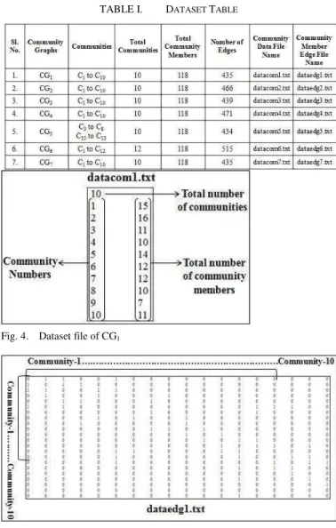
For the seven examples of community graphs, two sets of dataset files were created for each example of community graphs. The 1st dataset file contains community graph details such as number of communities, community number, and number of community members. So for the seven community graphs, these dataset files were from datacom1.txt to

datacom7.txt. Similarly the 2nd dataset file contains community graphs edge details i.e., edge between community members which only consist of 1s and 0s. So for the seven community graphs, these dataset files were from dataedg1.txt to

dataedg7.txt. These fourteen dataset file details are depicted in "Table I".

The algorithm was written in C++ and compiled with TurboC++ and run on Intel Core I5-3230M CPU +2.60 GHz Laptop with 4GB memory running MS-Windows 7. The comparison results of CG1 with CG2 to CG7 are depicted from

"Fig. 6" to "Fig. 17".

The datasets for community graphs CG1 to CG7 are in text

files from datacom1.txt to datacom7.txt and for datacom1.txt is depicted in "Fig. 4", which contains the total number of communities, community numbers, and a total number of community members. Similarly, the datasets for community graphs CG1 to CG7 are in text files from dataedg1.txt to dataedg7.txt and for dataedg1.txt is depicted in "Fig. 5", which contains the edge details, i.e., 0s (no edge) and 1s (edge) between the community members of similar communities as well as dissimilar communities of the community graphs.

TABLE I. DATASET TABLE

Fig. 4. Dataset file of CG1

Fig. 5. Dataset of CG1 contains edge details of community members C1 to C10

The authors have studied the existing techniques of Danai Koutra et al. method [1], Sergey Melnik et al. method [2], Glen Jeh et al. method [12], L Zager et al. method [13], and Hans-Peter Kriegel et al. method [14] for graph similarity.

In Danai Koutra et al. method [1], two graphs G1(N1, E1)

and G2(N2, E2), with possibly different number of nodes and

edges for similarity check, then adopting belief propagation (BP) into the proposed method for finding similarity between two graphs which finally returns a similarity value i.e., a real number between 0 and 1.

(6)

In Glen Jeh et al. method [12], to find similarity between two objects based on their relationships. Two objects are said to be similar, if they are related to similar objects. This similarity measure is called SimRank. This method is based on the simple graph-theoretic model.

In L Zager et al. method [13], it is a node-edge coupling, i.e., two graph elements is similar if their neighborhoods are similar. So edge score is constructed "when an edge in G1 is

like an edge in G2 if their respective source and terminal nodes

are similar". This is called edge similarity.

In Hans-Peter Kriegel et al. method [14], attributed graphs are considered as a natural model for the structured data. The authors proposed a new similarity measure between two attributed graphs, called "matching distance". The matching distance is calculated by sum of the cost for each edge matching.

The proposed method in this paper is different from the above existing methods. In the proposed method two community graphs with possibly equal number of nodes (communities) and different number of edges for similarity check. Each node (community) is labeled with a unique community number. Based on the community number of node, the similarity measure takes place by considering the weight of self-loop of community as well as the weight of edge between the communities. After similarity between two community graphs, it finally returns a similarity value i.e., a number from 0 to 3. Based on this number, the similarity of two community graphs can be judged. The proposed algorithm has capable of showing similarity and five different ways of dissimilarity. The five different dissimilarities are "similar on dissimilar edges", "similar on similar edges", "communities same but different edges", "communities not same", and "number of communities are different". Moreover, the proposed method is completely based on labeled community graphs and simple graph-theoretic model. So the authors conclude that the proposed community graph similarity is simply different from the above existing methods and fast since the time complexity is O(n3).

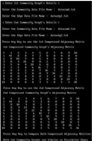
A. Comparison of CG1 and CG2

Fig. 6. (a) Community Graph CG1 (b) Community Graph CG2

In community graph CG1, the community codes (numbers)

are {C1, C2, C3, C4, C5, C6, C7, C8, C9, C10} with total

community members are {15, 16, 11, 10, 14, 12, 12, 10, 7, 11}. The total number of edges belonging to same community codes member are {44, 50, 26, 28, 36, 36, 34, 24, 20, 38}. Similarly, the total number of edges belonging to dissimilar community

codes member are C1-C2:8, C1-C4:9, C1-C5:3, C2-C3:9, C2-C5:5,

C2-C6:4, C3-C6:2, C3-C7:7, C4-C5:6, C4-C9:4, C5-C6:7, C5-C9:3,

C5-C10:3, C6-C7:9, C6-C8:3, C6-C10:5, C7-C8:4, C8-C10:5, and

C9-C10:3.

community members are {15, 16, 11, 10, 14, 12, 12, 10, 7, 11}. The total number of edges belonging to same community codes member are {44, 46, 24, 32, 42, 42, 38, 28, 26, 46}. Similarly, the total number of edges belonging to dissimilar community codes member are C1-C2:8, C1-C4:9, C1-C5:3, C2-C3:9, C2-C5:5,

C2-C6:4, C3-C6:2, C3-C7:7, C4-C5:6, C4-C9:4, C5-C6:7, C5-C9:3,

C9-C10:3.

The comparison takes place on community graph CG1 and

CG2’s community codes and the number of edges belonging to

dissimilar community codes member since these two are same. So finally the algorithm shows as "Both the Community Graphs are Similar on Dissimilar Edges".

(7)

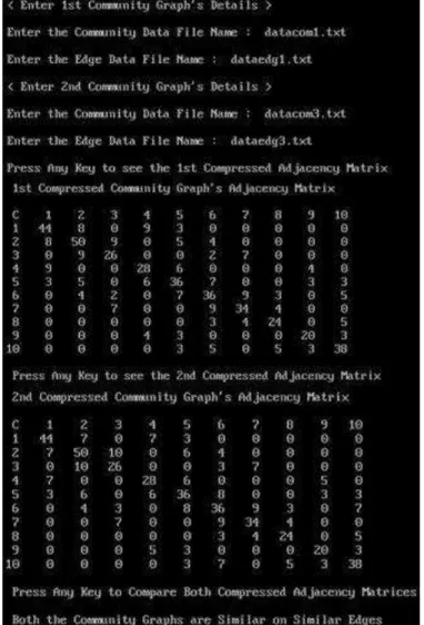
B. Comparison of CG1 and CG3

Fig. 8. (a) Community Graph CG1 (b) Community Graph CG3

Fig. 9. Comparison result of CG1 and CG3

C2-C6:4, C3-C6:2, C3-C7:7, C4-C5:6, C4-C9:4, C5-C6:7, C5-C9:3,

C9-C10:3.

community members are {15, 16, 11, 10, 14, 12, 12, 10, 7, 11}. The total number of edges belonging to same community codes member are {44, 50, 26, 28, 36, 36, 34, 24, 20, 38}. Similarly, the total number of edges belonging to dissimilar community codes member are C1-C2:7, C1-C4:7, C1-C5:3, C2-C3:10, C2

-C5:6, C2-C6:4, C3-C6:3, C3-C7:7, C4-C5:6, C4-C9:4, C5-C6:8, C5

-C9:3, C5-C10:3, C6-C7:9, C6-C8:3, C6-C10:7, C7-C8:4, C8-C10:5,

and C9-C10:3.

CG3’s community codes and the number of edges belonging to

similar community codes member since these two are same. So finally the algorithm shows as "Both the Community Graphs are Similar on Similar Edges".

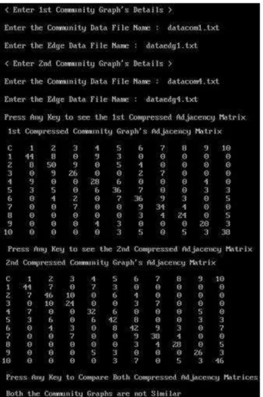
C. Comparison of CG1 and CG4

Fig. 10.(a) Community Graph CG1 (b) Community Graph CG4

C2-C6:4, C3-C6:2, C3-C7:7, C4-C5:6, C4-C9:4, C5-C6:7, C5-C9:3,

C9-C10:3.

-C5:6, C2-C6:4, C3-C6:3, C3-C7:7, C4-C5:6, C4-C9:5, C5-C6:8, C5

-C9:3, C5-C10:3, C6-C7:9, C6-C8:3, C6-C10:7, C7-C8:4, C8-C10:5,

and C9-C10:3.

CG4’s number of edges belonging to similar community codes

(8)

Fig. 11.Comparison result of CG1 and CG4

D. Comparison of CG1 and CG5

In community graph CG1, the community codes (numbers) are {C1, C2, C3, C4, C5, C6, C7, C8, C9, C10} with total

C2-C6:4, C3-C6:2, C3-C7:7, C4-C5:6, C4-C9:4, C5-C6:7, C5-C9:3,

C9-C10:3.

-C6:5, C5-C8:4, C10-C8:2, C10-C11:2, C4-C6:6, C4-C12:4, C6-C8:7,

C4-C12:3, C6-C13:3, C8-C11:9, C8-C7:3, C8-C13:5, C11-C7:4, C7

-C13:5, and C12-C13:3.

CG5’s community codes. Since the community codes of

community graphs CG1 and CG5 are not same. So the

algorithm shows as "Both the Community Graphs are not Similar".

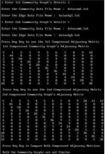
E. Comparison of CG1 and CG6

(9)

the total number of edges belonging to dissimilar community codes member are C1-C2:8, C1-C4:9, C1-C5:3, C2-C3:9, C2-C5:5,

C2-C6:4, C3-C6:2, C3-C7:7, C4-C5:6, C4-C9:4, C5-C6:7, C5-C9:3,

C9-C10:3.

are {C1, C2, C3, C4, C5, C6, C7, C8, C9, C10, C11, C12} with total

community members are {15, 16, 11, 10, 14, 12, 12, 10, 7, 11, 9, 11}. The total number of edges belonging to same community codes member are {44, 50, 26, 28, 36, 36, 34, 24, 20, 38, 26, 38}. Similarly, the total number of edges belonging

to dissimilar community codes member are C1-C2:8, C1-C4:8,

C1-C5:3, C2-C3:9, C2-C5:5, C2-C6:4, C3-C6:2, C3-C7:7, C4-C5:6,

C4-C9:4, C5-C6:7, C5-C9:3, C5-C10:3, C6-C7:9, C6-C8:3, C6

-C10:5, C7-C8:4, C8-C10:5, C8-C12:2, C9-C10:3, C9-C11:2, C10

-C11:4, C10-C12:4, and C11-C12:5.

CG6’s community codes. Since the number of community

codes of community graphs CG1 and CG6 are not same. So the

algorithm shows as "Both the Community Graphs are not Similar".

F. Comparison of CG1 and CG7

(10)

C2-C6:4, C3-C6:2, C3-C7:7, C4-C5:6, C4-C9:4, C5-C6:7, C5-C9:3,

C9-C10:3.

C2-C5:5, C1-C5:3, C1-C4:9, C7-C6:9, C7-C8:4, C6-C5:7, C6-C8:3,

C10-C9:3.

CG7’s community codes. Since the community codes of

community graphs CG1 and CG7 are same. Then the

comparison takes place on a number of edges belonging to similar community codes member and number of edges belonging to dissimilar community codes member. So finally the algorithm shows as "Both the Community Graphs are Similar".

VI. CONCLUSIONS

Graph similarity technique is helpful in the fields of shape retrieval, object recognition, face recognition and many more areas. This paper starts with literature survey related to various techniques implemented for graph similarity. So it is important to compare two community graphs for similarity check to extract the reliable knowledge from a large community graph. This paper proposes an algorithm for similarity check of two community graphs using graph mining techniques. The authors have implemented the proposed algorithm using C++ programming language and obtained satisfactory results.

REFERENCES

[1] Danai Koutra, Ankur Parikh, Aditya Ramdas, and Jing Xiang, "Algorithms for Graph Similarity and Subgraph Matching," Dec 4, 2011. https://www.cs.cmu.edu/~jingx/docs/DBreport.pdf

[2] B. Huet, A. Cross, and E. Hancock, "Shape retrieval by inexact graph matching." in Proc. IEEE Int. Conf. on Multimedia Computing Systems. Volume 2., IEEE Computer Society Press, 1999, pages 40–44. [3] E. Kubicka, G. Kubicki, and I.Vakalis, "Using graph distance in object

recognition." in Proc. ACM Computer Science Conference, 1990, pages 43–48.

[4] L. Wiskott, J. M. Fellous, N. Kr¨uger, and C. Von Der Malsburg, "Face recognition by elastic bunch graph matching." in IEEE PAMI 19, 1997, pages 775–779.

[5] V. Levenshtein. "Binary codes capable of correcting deletions, insertions and reversals," in Soviet Physics Doklady(10), 1966, 707–710. [6] R. A. Wagner and M. J. Fisher, "The string-to-string correction

problem," in Journal of the ACM(21), 1974, 168–173.

[7] A. Sanfeliu and K. S. Fu, "A distance measure between attributed relational graphs for pattern recognition," in IEEE Transactions on Systems, Man and Cybernetics(13), 1983, 353–362.

[8] D. J. Cook and L. B. Holder, "Graph-based data mining," in IEEE Intelligent Systems (15), 2000, 32–41.

[9] Duncan J. Watts, "Small worlds: the dynamics of networks between order and randomness", Princeton University Press, 1999.

[10] Sung-Hyuk Cha, "Comprehensive survey on distance/similarity measures between probability density functions," in International Journal of Mathematical Models and Methods in Applied Sciences, 1(4), 2007, 300–307.

[11] Sergey Melnik, Hector Garcia-Molina, and Erhard Rahm, "Similarity

ﬂooding: A versatile graph matching algorithm and its application to schema matching," in 18th International Conference on Data Engineering (ICDE 2002), 2002.

[12] Glen Jeh and Jennifer Widom, "SimRank: A measure of structural-context similarity," in Proceedings of the eighth ACM SIGKDD International Conference on Knowledge Discovery and Data Mining,

KDD ’02, New York, USA, 2002, pages 538–543.

[13] L. Zager and G. Verghese, "Graph similarity scoring and matching," in Applied Mathematics Letters, 21(1), 2008, 86–94.

[14] Hans-Peter Kriegel and Stefan Schonauer, "Similarity Search in Structured Data," in Proceedings 5th International Conference on Data

Warehousing and Knowledge Discovery (DaWaK’ 03), Prague, Czech

Republic, 2003, pages 224-233.

[15] Jonathan S. Yedidia, William T. Freeman, and Yair Weiss, "Understanding belief propagation and its generalizations," in Morgan Kaufmann Publishers Inc., San Francisco, CA, USA, 2003, pages 239– 269.

[16] Bapuji Rao, Anirban Mitra and D. P. Acharjya, "A New Approach of Compression of Large Community Graph Using Graph Mining Techniques," in Proceedings of 3rd ERCICA 2015, Volume 1, Springer Verlag, NMIT, Bangalore, India, Pp. 127 – 136, July 31–Aug 1, 2015. DOI: 10.1007/978-81-322-2550-8_13