Adilson de Jesus Martins da Silva
Master of ScienceVariance Components Estimation In Mixed
Linear Models
Dissertação para obtenção do Grau de Doutor em Estatística e Gestão de Risco
Orientador:
Miguel dos Santos Fonseca, Investigador,
Universidade Nova de Lisboa
Co-orientadores:
Dário Ferreira, Prof. Auxiliar,
Universidade de Beira Interior
Francisco Carvalho, Prof. Adjunto,
Instituto Politécnico de Tomar
Júri:
Presidente: Prof. Doutor Fernando José Pires Santana Arguentes: Prof. Doutor Martin Singull
Prof. Doutora Célia Maria Pinto Nunes Vogais: Prof. Doutor Kamil Feridun Turkman
Prof. Doutora Maria Manuela Costa Neves Figueiredo Prof. Doutora Isabel Cristina Maciel Natário
Variance Components Estimation In Mixed Linear Models
Copyright cAdilson de Jesus Martins da Silva, Faculdade de Ciências e Tecnologia, Universidade Nova de Lisboa
A
CKNOWLEDGEMENTS
First, i wish to express my sincere and deep gratitude to my supervisor, researcher Dr. Miguel Fonseca for his encouragement and guidance throughout my research for this thesis. He provided intellectual stimulation and emotional support for this research, but just as importantly, he provided insight into what it means to be a professional theoretical statistician. To my co-supervisors, Prof. Dr. Dário ferreira and Prof. Dr. Francisco Carvalho, i also express my deep gratitude for their support, contributes, and constructive comments on this thesis. I want to thank Prof. Dr. João Tiago Mexia for its suggestion early when i was at the beginning of my research, encouraging me, together with my adviser, to pick the topic i investigated for this thesis.
I wish to express my especial gratitude to the “Fundação Calouste Gulbenkian” for the support through a PhD grants.
I’m particularly indebted to my parents Miguel and Cipriana; their personal belief in the value of knowledge and education instilled in my siblings and me early in life has been a continuing force in my graduate and postgraduate programs. I’m thankful to my brothers Tila, Zamy, Du, viró, Vany, and Deisy for their encouragement for this important step in my academic career. I’m also in debt to my uncle Eduardo for all his support throughout my academic route; without him it would not be possible.
A
BSTRACT
This work aim to introduce a new method of estimating the variance components in mixed linear models. The approach will be done firstly for models with three variance components and secondly attention will be devoted to general case of models with an arbitrary number of variance components.
In our approach, we construct and apply a finite sequence of orthogonal transformations, here named sub - diagonalizations, to the covariance structure of the mixed linear model producing a set of Gauss-Markov sub-models which will be used to create pooled estimators for the variance components. Indeed, in order to reduce the bias, we apply the sub - diagonalizations to its cor-respondent restricted model, that is its projection onto the orthogonal subspace generated by the columns of its mean design matrix. Thus, the Gauss - Markov sub-models will be centered. The produced estimator will be calledSub-D.
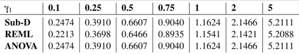
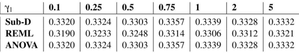
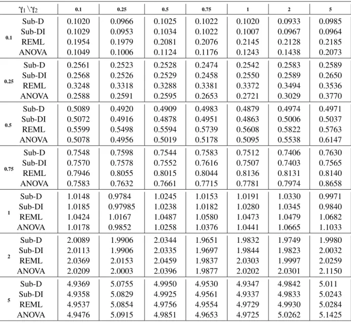
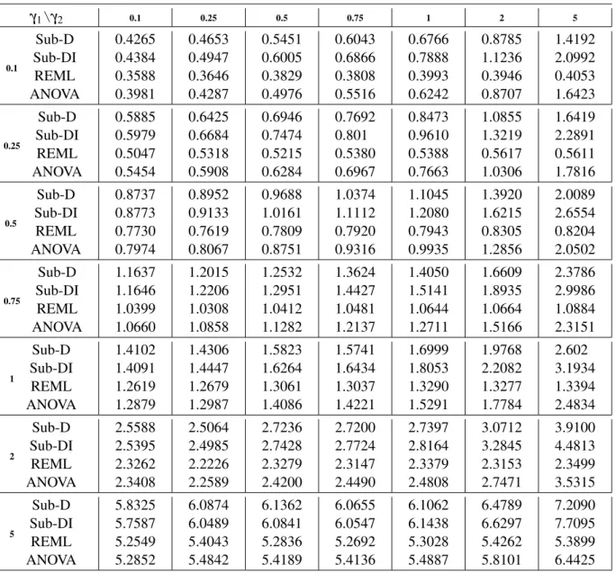
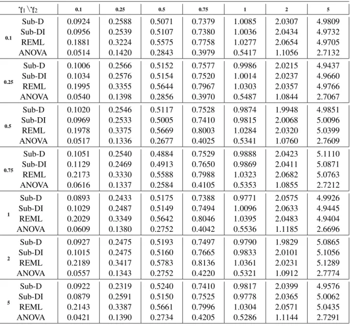
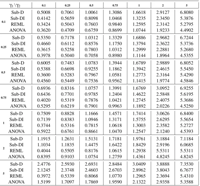
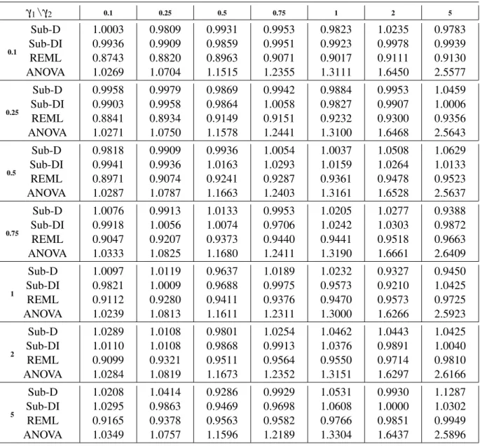
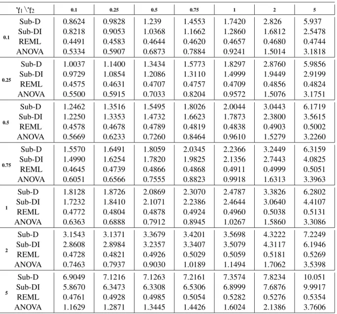
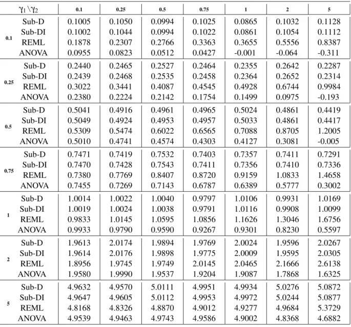
Finally, the numerical behavior of the proposed estimator is examined for the case of models with three variance components, comparing its performance to the ones obtained with the REML and ANOVA estimators. Numerical results show thatSub-Dproduces reasonable and comparable estimates, some times slightly better than those obtained with REML and mostly better than those obtained with ANOVA.
Due to the correlation between the sub-models, the estimated variability of the variability of
Sub-Dwill be slightly bigger than the one of the REML estimator. In attempt to solve this problem
a new estimator will be introduced.
R
ESUMO
Este trabalho pretende introduzir um novo método de estimação das componentes da variância em modelos lineares mistos. Numa primeira instância, aborda-se a estimação em modelos com três componentes da variância. Seguidamente, foca-se no caso geral: estimação em modelos com um número arbitrário de componentes da variância.
Na nossa abordagem, construimos e aplicamos uma sequência finita de transformações ortogo-nais - aqui denominadas sub-diagonalizadoras - à estrutura da covariância do modelo, produzindo assim um conjunto de sub - modelos de Gauss-Markov que serão usados para criar estimadores agrupados. Na verdade, com o intuito de reduzir o viés, aplicamos as sub-diagonalizadoras ao modelo restrito correspondente, isto é, à projeção do complemento ortogonal no subspaço gerado pelas colunas da sua matriz do delineamento para a esperança (parte dos efeitos fixos), pelo que os sub-modelos de Gauss-Markov acima referidos terão média nula. O estimador resultante será chamado deSub-D.
Finalmente, examina-se o desempenho numérico do estimador proposto para o caso do modelo com três componentes da variância, comparando-o com o dos estimadores REML e ANOVA. Os resultados obtidos mostram que o nosso estimador (Sub-D) produz estimativas razovelmente comparáveis, sendo, em alguns casos, ligeiramente melhores que os resultados obtidos com o estimador REML e na maioria dos casos melhores que os obtidos com o estimador ANOVA. Contudo, devido à dependência entre os sub-modelos, a variabilidade estimada será ligeiramente maior que a do estimador REML. Na tentativa de ultrapassar esse problema um novo estimador será introduzido.
C
ONTENTS
List of Notations and Abbreviations xv
1 Introduction 1
2 Algebraic Results 3
2.1 Notation And Preliminary Notions On Matrix Theory . . . 3
2.1.1 Diagonalization Of A Symmetric Matrix . . . 8
2.2 Orthogonal Basis And Projection Matrices . . . 11
2.2.1 Application To Statistics . . . 14
2.3 Generalized Inverses . . . 16
2.3.1 Moore-Penrose Inverse . . . 18
2.4 Jordan Algebras . . . 20
2.5 Kronecker Product . . . 25
3 Mixed Linear Models 29 3.1 Variance Components Estimation - ANOVA Method . . . 34
3.2 Variance Components Estimation - Likelihood Aproach . . . 36
3.2.1 ML - Based Method . . . 37
3.2.2 REML - Based Method . . . 38
3.3 Variance Components Estimation - Models With OBS . . . 40
4 Variance Components Estimation - The Sub-D Method 43 4.1 Introduction And Literature Review . . . 43
4.1.1 Designs For Variance Components Estimation . . . 43
4.1.2 Procedures For Variance Components Estimation . . . 45
4.2 Sub-Diagonalizing The Variance-Covariance Matrix . . . 46
4.2.1 The Caser=2 . . . 47
4.2.2 Estimation Forr=2 . . . 52
4.2.3 The General Case:r≥1 . . . 56
4.2.4 The General case: Estimation Forr≥1 . . . 61
4.3 Improving The Sub-D Estimator . . . 64
5.2 The Performance I: “One-Way Design” . . . 68
5.2.1 Balanced “One Way Design” . . . 69
5.2.2 Unbalanced “One-Way Design” . . . 70
5.3 The Performance II: “Two-Way Crossed Design” . . . 71
5.4 The Performance III: “Two-Way Nested Design” . . . 73
6 Final Coments 87 A Appendix 89 A.1 Useful Results . . . 89
A.1.1 Algebraic Results . . . 89
A.1.2 Statistical Results . . . 90
L
IST OF
N
OTATIONS AND
A
BBREVIATIONS
Mn×m Set of matrices of sizen×m
Sn Set of symmetric matrices with sizen×n 0n,m Null matrix of sizen×m
0n Null vector of sizen 1n Vector of 1’s of sizen
Jn,m Matrix of 1’s of sizen×m
In Identity matrix of sizen
X−1 Inverse of matrixX
X− Generalized inverse of matrixX X+ Moore-Penrose inverse of matrixX X⊤ Transpose of matrixX
r(X) Rank of matrixX tr(X) Trace of matrixX
R(X) Vector space spanned by the column vectors of matrixX N(X) Kernel of matrixX
R(X)⊥ Orthogonal complement ofR(X)
PR(X) Projection Matrix ontoR(X) E(y) Expectation of the random vectory
Σ(x,y) Cross-covariance between the random vectorsxandy Σ(y) Variance-covariance of the random vectory
Var(y) Variance of the random variabley
y∼(Xµ, Σ) yis a vector with expectationXµ and variance-covariance matrixΣ
y∼N (Xµ, Σ) yis a normal random vector with mean vectorXµ and variance-covariance matrixΣ
ML Maximum Likelihood
REML Restricted Maximum Likelihood ANOVA Analysis of Variance
C
H
A
P
T
E
R
1
I
NTRODUCTION
Mixed linear models (MLM) have received much attention recently, namely because they constitute an useful tool for modeling repeated measurement data, and, in particular, small sample and longitudinal data (Wallace and Helms [27] developed procedures providing hypothesis tests and confidence intervals for longitudinal data using MLM).
MLM arise due to the necessity of accessing the amount of variation caused by certain sources in statistical designs with fixed effects (see Khuri [34]) for example the amount of variation that are not controlled by the experimenter and those whose the levels are randomly selected from a large population of levels. The variances of such sources of variation, currently refereed to as variance components, have been widely investigated mainly in the last fifty years of the last century (see Khuri and Sahai [35], Searle ([65], [66]), for example), and thanks to the proliferation of research in applied areas such as genetic, animal and plant breeding, statistical process control and industrial quality improvement (see Anderson ([2], [4], [3]), Anderson and Crump [6], Searle [65] for instance) several techniques of estimation for the variances components have been proposed. Among them we highlight the ANOVA and likelihood based method (see Searle at al. [67] and Casella and Berger [14]), as well as those based on orthogonal block structure (OBS) (see Nelder ( [57], [58]). Nevertheless, notwithstanding the ANOVA method adapt readily to mixed models with balanced data and save the unbiasedness, it does not adapt in situation with unbalanced data (mostly because it uses computations derived from fixed effect models rather than mixed models). On its turn, the maximum likelihood - based methods provide estimators with several statistical optimal properties such as consistency and asymptotic normality either for models with balanced data, or for those with unbalanced data. For these optimal properties we recommend, for instance, Miller ( [46], [47]) and for some details on applications of such methods we suggest Anderson [4] and Hartley and Rao [25]. The OBS based method plays important role in the theory of randomized block designs (see Calinski and Kageyama ([12], [13])).
to general case of models with an arbitrary number of variance components. In our approach, in order to reduce the bias of our estimator, we will instead consider the orthogonal projection of the normal MLM onto the subspace generated by the columns of its correspondent mean design matrix, that is the restricted model. We construct and apply a finite sequence of orthogonal matrices to the covariance structure of the restricted model thus producing a set of homoscedasticity sub-models and then use that sub-models structure to developing the above announced estimator. For now on the finite sequence of orthogonal matrices will be refereed to as sub-diagonalizations, and the estimators developed here refereed to asSub-DandSub-DI, whereSub-DIis found in an attempt to improve theSub-D. Through this work sometimes we may have the need to refer to the underlying deduction method ofSub-Dand sometimes to the deducted estimator; when so, for the first case we will refer to asSub-Dmethod, whereas for the second one asSub-Destimator.
C
H
A
P
T
E
R
2
A
LGEBRAIC
R
ESULTS
In this chapter we will review the elements of matrix theory needed in the remainder of the thesis, especially in both chapter 3 and 4. The proofs of the results that seem, somehow, instructive will be included. On the other hand, for the proofs of the remainder results we will always include some references. Among them, we highlight Schott [64], Rao and Rao [61], and Rencher and Schaalje [62].
We begin with the presentation of some basic notions onmatrix theoryin section 2.1 and next we present results onorthogonal basisandprojection matrices(section 2.2), followed by a brief presentation and discussion ofdiagonalizationof asymmetric Matrix. In section 2.3 thegeneralized
inverse matrix notions and some important results for the remainder chapter (see section 2.3).
Finally, at the last two sections (sections 2.4 and 2.5) discussion of needed notions and results on
Jordan algebraand onKronecker productof matrices follow.
2.1
Notation And Preliminary Notions On Matrix Theory
Throughout this work we use the capital letter to represent a matrix and, when needed, the lower case letter to represent a vector. LetMn×mstands for the set of matrices withnrows andmcolumns. Thereby, withA∈Mn×mwe mean a matrix whose the dimension is characterized bynrows andm columns, and the element in the row 0<i≤nand column 0< j≤m, that is, the(i,j)thelement,
is a scalars or a variable, usually denoted byai j. Let
A=
a11 a12 . . . a1m
a21 a22 . . . a2m ..
. ... . .. ...
an1 an2 . . . anm
, (2.1)
Interchanging the rows and columns of A∈Mn×m the resulting matrix is said to be the
transpose matrixofAand is denoted byA⊤; that is,A⊤is a matrix whose the element at rowiand
column jis exactly the element at row jand columniof matrixA. So,
A⊤=
a11 a21 . . . an1
a12 a22 . . . an2
..
. ... . .. ...
a1m a2m . . . anm
.
Ifn=m,Ais said to be asquare matrixand whenAis asquare matrixwithai j =0, fori6= j,
Ais said to be adiagonal matrix. Here we denote it byD(a11,. . .,ann)or justDwhen there is no risk of misunderstanding. Whenai j =0, for alliand j,Ais called anull matrix. We will represent a null matrix by0n,m.
Throughout this work we will assume the following notation for some especial matrices (including the vectors):
• 0ndenotes a vector inRnwhose the entries are all equals to 0;
• Jn,mdenotes a matrix in∈Mn×mwhose the entries are all equals to 1; whenn=mit will be denotedJn;
• 1ndenotes a vector inRnwhose the entries are all equals to 1.
Adiagonal matrix Awhose the diagonal elements are all equal to one is calledidentity matrix.
We will denote it here byIn, or justIwhen there is no risk of misunderstanding.
Definition 2.1.1. LetA∈Mn×n; that is, asquare matrix.Ais said to be asymmetric matrixif it holdsA⊤=A. Here we denote the set of allsymmetric matricesinMn×nbySn.
For what follows it is assumed that the reader is familiarized with sum and product of matrices (if not, see Lay [38] for instance). We will introduce several functions of matrix and discuss a few of them, mainly those with direct implication on the remainder chapters. For this latter ones we will present the notions and the main results. for the remaining ones we recommend Lay [38] or Schott [64], for instance.
One of the matrix function with no direct implication in this work is| |, thedeterminantof a
square matrix(see Horn and Johnson [30] for this topic). Given asquare matrix A, if|A| 6=0,Ais said to be anon-singular matrix. See Schott [64] or Lay [38] for more explanation.
Another function defined over asquare matrixis thetracefunction.
Definition 2.1.2. LetA∈Mn×n. ThetraceofA, denoted bytr(A), is defined by
tr(A) =
n
∑
s=1ass;
2.1. NOTATION AND PRELIMINARY NOTIONS ON MATRIX THEORY
Thetracefunction plays an important role on statistic field, with some emphasis, for example,
on the distribution of quadratic forms (see Schott [64] or Rencher and Schaalje [62]). Indeed, given a random vectory∈Rnwith mean vectorµ and variance-covariance matrixΣ, and asymmetric
matrix A∈Mn×n, the expectation of the quadratic formy⊤Ay, denoted byE(y⊤Ay), is given by
E(y⊤Ay) =tr(AΣ) +µ⊤Σµ. (2.2)
Ifyhas finite fourth moment, we have that the variance-covariance matrix of y⊤Ay, denoted by Σ(y⊤Ay), is given by
Σ(y⊤Ay) =2tr([AΣ]2) +2µ⊤AΣAµ. (2.3)
The following result summarizes a few useful properties of thetracefunction. Proposition 2.1.1. Let A,B∈Mn×nandα∈R. Then
(a) tr(A⊤) =tr(A);
(b) tr(A+αB) =tr(A) +tr(αB) =tr(A) +αtr(B);
(c) tr(AB) =tr(BA);
(d) tr(A⊤A) =0n,nif and only if A=0n,n.
Proof. For(a)we only have to note that the diagonal element ofAare the same as those ofA⊤. For
(b), withδii,i=1,. . .,n, denoting the diagonal elements ofA+αBit follows thatδii=aii+αbii, whereaiiandbiidenote the the diagonal elements ofAandB, respectively. For(c), letAi•andA•j respectively denote theith row and the jth column of the matrixA. Thus the elementci j ofC=AB will be
ci j=Ai•B•j = n
∑
k=1aikbik
and the elementdi jofD=BAwill be
di j=Bi•A•j= n
∑
k=1bikaik.
tr(AB) = tr(C) =
n
∑
i=1cii= n
∑
i=1Ai•B•i= n
∑
i=1n
∑
k=1aikbki= n
∑
k=1n
∑
i=1bkiaik= n
∑
k=1Bk•A•k= n
∑
k=1dkk
= tr(D) =tr(BA).
Finally, for(d), the sufficient condition is obviously onceA=0n,nimpliesA⊤A=0n,n. Now, for the necessary condition, withE=A⊤and nothing thatEi•=A•i, we will have
tr(A⊤A) =
n
∑
i=1Ei•A•i= n
∑
i=1n
∑
k=1eikaki= n
∑
i=1n
∑
k=1a2ki. (2.4)
Consequently,tr(A⊤A) =0 holds if and only ifaki=0 for allk and alliwhich means exactly
Definition 2.1.3. LetA∈Mn×nbe anon-singular matrix. The unique matrixBsuch that
BA=AB=In
is called theinverse matrixof matrixA, and denoted byA−1.
As seen we gave the above notion presupposing the existence and the uniqueness of theinverse
of anon-singular matrix. The proofs for these facts can be explored at Schottt [64].
Next we summarize a few basic useful properties of the inverse of a matrix in the following proposition. They all can be easily proved using the above definition.
Proposition 2.1.2. Let A,B∈Mn×nbe non-singular matrices, andα a nonzero scalar.
(a) (αA)−1= 1
αA−1;
(b) (A⊤)−1= A−1⊤
;
(c) (A−1)−1=A;
(d)
A−1
= 1
|A|;
(e) If A is symmetric, then A−1is symmetric; that is, A−1= (A−1)⊤;
(f) (AB)−1=B−1A−1;
(g) If A=D(a11,. . .,ann), then A−1=D
1
a11,
. . ., 1
ann
.
Proof. See Schott [64], Theorem 1.6.
Now we turn to what we may call inside structure of a matrix. Specifically, we will reveal a few interesting and useful properties hidden in the matrix columns (rows).
Since each of themcolumns of a matrixA∈Mn×mhasnentries they may be identified with
vectors inRnso that we may writeA= [v
1. . .vm], wherevi=
a1i .. .
ani
,i=1,. . .,m. It is easily noted
that the linear combination of the column vectors ofAcan be written as a product ofAwith a vector
x∈Rm:Ax=x
1v1+. . .+xmvm, wherex=
x1
.. .
xm
.
Definition 2.1.4. The set of all possible linear combination of the column vectorsv1,. . .,vmofAis called therangeofA, and denoted byR(A); that is, withx= [x1. . .xm]⊤representing any vector of realsxi,
R(A) ={v∈Rn:Ax=v} ⊂Rn.
Definition 2.1.5. The set of all vectorw∈Rmsuch thatAw=0 is called thenull spaceofA, and denoted byN(A); that is,
2.1. NOTATION AND PRELIMINARY NOTIONS ON MATRIX THEORY
As it may be noted, R(A)and N(A) are vector subspace of the vector spacesRn and Rm, respectively (see Schott [64]). We prove it on the next result.
Proposition 2.1.3. Let A∈Rn×m. Then
(a) R(A)is a vector subspace ofRn;
(b) N(A)is a vector subspace ofRm;
Proof.
(a):0n∈R(A), sinceA0m=0n. Ifv,w∈R(A), we have thatAx=vandAy=wfor some vectorsx,y∈Rm. Thus,A(x+y) =Ax+Ay=v+wso thatv+w∈R(A). Finally, letα be an scalar andv∈R(A). Then, sincev=Axfor some vectorx∈Rm, andA(αx) =α(Ax) =αv, we have thatαv∈R(A)and so the proof for this part is completed; that isR(A)is a vector subspace.
(b):0m∈N(A), sinceA0m=0n. Lettingv,w∈N(A)we have thatAv=0nandAw=0n. Then,
A(v+w) =Av+Aw=0nand, therefore,v+w∈N(A). Finally, for any scalarα andv∈N(a)we will have thatA(αv) =α(Av) =0nso thatαv∈N(A)and so the proof is completed; that isN(A) is a vector subspace.
Definition 2.1.6. The dimension ofR(A)is called therankofA. We denote it here byr(A). The following theorems summarize a set of useful results onmatrix rank. Some of them will play important role in the chapter 4 (which we may call this work main contributes), since they will have direct implication (either they justify some steps, or taken as consequence) on the proofs for the most important results on that chapter.
Theorem 2.1.4. Let A∈Mn×m. Then
(a) r(A)and the dimension of the row space of A are equal; that is, r(A) =r(A⊤);
(b) r(A)+ dimN(A) =m, where dimN(A)denotes the dimension of N(A).
(c) If n=m and A is a diagonal matrix, then r(A) =r, where r is the number of its nonzero
diagonal elements.
Proof. For the proof of(a)and(b)see Lay [38].(c)is a direct consequence of the definition.
Theorem 2.1.5. Let A∈Mn×m, B∈Mn×nand C∈Mm×mbe non-singular matrices. Then
(a) r(A) =r(A⊤) =r(A⊤A) =r(AA⊤);
(b) r(BAC) =r(BA) =r(AC) =r(A).
Proof. See Schott [64], Theorems 1.8 and 2.10.
Theorem 2.1.6. Let Ai∈Mn×m, i=1, 2, and B∈Mm×p. Then
(a) r(A1+A2)≤r(A1) +r(A2);
(b) r(A1B)≤min{r(A1),r(B)}.
2.1.1 Diagonalization Of A Symmetric Matrix
In this section we present some brief notions ofeigenvaluesandeigenvectors(which are solutions of a specific equation of matrix functions) and then discuss a few important results concerning this subject as well as some others connecting it withmatrix rank. This concepts are defined over a
square matrix. The latter part of this section is devoted to a discussion on the diagonalization of
symmetric matrix, specifically, the spectral decomposition of a matrix. Definition 2.1.7. LetA∈Mn×n. Any scalarλ such that
(A−λIn)v=0, (2.5)
for some non-null vectorv∈Rn, is called aneigenvalueofA. Such a non-null vectorvis called the
eigenvectorofAand equation (2.5) theeigenvalue-eigenvectorequation.
Sincev6=0, it must be noted that theeigenvalueλ must satisfy the determinant equation
|A−λIn|=0 (2.6)
which is known as characteristic equation ofAsince using the definition of determinant function (see Schott [64]) it can be equivalently written as
θo−θ1λ+. . .+θn−1(−λ)n−1+ (−λ)n=0, (2.7)
for some scalarsθi,i=0,. . .,n−1, that is, as annthdegree polynomial inλ. Theorem 2.1.7. Let A∈Mn×n. Then
(a) λ is eigenvalue of A if and only ifλ is eigenvalue of A⊤;
(b) A is non-singular if and only if A has no null eigenvalues;
(c) If B∈Mn×nis a non-singular matrix, then the eigenvalues of BAB−1are the same as the
those of A;
(d) |A|is equal to the product of the eigenvalues of A.
Proof. straightforward using the characteristic equation or the eigenvalue-eigenvector equation.
It is known that the polynomial in the left side of (2.7) has at mostnreal roots (and exactly
ncomplex roots); that is, there are at mostnscalar,λ1,. . .,λnsay, satisfying the equation (2.7) if solved inλ, so thatAhas at mostnreal eigenvalues.
Theorem 2.1.8. Let A∈Snand B∈Mn×n. Then
(a) The set of eigenvectors associated to different eigenvalues of B are linearly independent.
(b) Letλ1,. . .,λs, s≤n, be the eigenvalues of A. Thenλ1,. . .,λsare all reals, and for eachλi,
2.1. NOTATION AND PRELIMINARY NOTIONS ON MATRIX THEORY
(c) It is possible to construct a set of eigenvectors of A such that the set is orthonormal; that is
each element in the set has euclidean norm equal to one and they are pairwise orthogonal.
Proof. (a): withr<n, supposeν1,. . .,νr are the eigenvectors ofA, and let the corresponding
eigenvaluesλ1,. . .,λrbe such thatλi6=λj, wheneveri6= j. Now suppose, by contradiction, that
ν1,. . .,νr are linearly dependent. Let h be the largest integer for whichν1,. . .,νh are linearly independent (that is,ν1,. . .,νh+1must be linearly dependent). Thus, since no eigenvector can be a
null vector, there exist scalarsα1,. . .,αh+1with at least two not equal to zero, such that α1ν1+. . .+αh+1νh+1=0n.
Premultiplying both the left-hand and the right-hand side of this equation by(A−λh+1In)it is found that
α1(A−λh+1In)ν1+. . .+αh+1(A−λh+1In)νh+1=0n ⇔
α1(Aν1−λh+1ν1) +. . .+αh+1(Aνh+1−λh+1νh+1) =0n ⇔
α1(λ1ν1−λh+1ν1) +. . .+αh+1(λh+1νh+1−λh+1νh+1) =0n ⇔
α1(λ1−λh+1)ν1+. . .+αh(λh−λh+1)νh=0n. (2.8)
Thus, sinceν1,. . .,νhare linearly independent it follows that
α1(λ1−λh+1) =···=αh(λh−λh+1) =0n.
Now, since at least one of the scalarsα1,. . .,αhis not equal to zero, for somei=1,. . .,hwe have thatλi=λh1, which contradicts the condition of(a).
(b): Letλ =α+iβ be an eigenvalue ofAandν=x+izits corresponding eigenvector, where
i=√−1. Thus, we have that
Aν=λ ν⇔A(x+iz) = (α+iβ)(x+iz), (2.9)
and premultiplying by(x−iz)⊤, it yields
(x−iz)⊤(x+iz) = (α+iβ)(x−iz)⊤(x+iz). (2.10)
HenceAis symmetric equation (2.10) simplifys to
x⊤Ax+z⊤Az= (α+iβ)x⊤x+z⊤z
. (2.11)
Sinceν6=0n(it is an eigenvector) we have that x⊤x+z⊤z
>0 and, consequently,β =0 since
the left-hand side of the equation (2.11) is real. Now, replacingβ with zero in the eigenvalue-eigenvector equation (2.9) we get
A(x+iz) =α(x+iz)⇔
Thenν=x+izwill be an eigenvector ofAcorresponding toλ =α as long asAx=αx,Az=αz
and at least one of the vectorsxandzmust be non-null (onceν6=0n). Finally, a real eigenvector corresponding toλ =α is then constructed by choosingx6=0nsuch thatAx=αxandz=0.
(c): Letνbe any non-null vector orthogonal to each of the eigenvectors in the set{ν1,. . .,νh}, where 1≤h<n. Note that the set{ν1,. . .,νh}contains at least one eigenvector ofA. Note also
that for any integerk≥1,Akνis also orthogonal to each of the vectors in the set since, ifλiis the eigenvalue corresponding toνi, it follows from the symmetry ofAand Theorem A.1.1 that
νi⊤Akν=Ak⊤νi
⊤
ν= (Akν
i)⊤ν=λikνi⊤ν=0.
According with the TheoremA.1.2 we have that the space spanned by the vectorsν,Aν,. . .,
Ar−1ν,r≥1, contains an eigenvector ofA. Let it beν∗. Clearlyν∗is also orthogonal to the vectors in the set{ν1,. . .,νh}, since it comes from a vector space spanned by a set of vectors which are orthogonalν1,. . .,νh. Thus we can takeνh+1= (ν∗⊤ν)
−1
2 . Then, starting with any eigenvector of
A, and proceeding with the same argumentn−1 times the theorem follows.
It must be noted that if the matrixA∈Mn×nhas 1<r≤neigenvaluesλ
1,. . .,λrwhose the corresponding eigenvectors will be the non-null vectorsv1,. . .,vr, i.e.(A−λi)vi=0,i=1,. . .,r, the eigenvalue - eigenvector equation can be written as
AV =VΛ or, equivalently,(AV−VΛ) =0n,r, (2.12)
whereV is a matrix inMn×rwhose the columns arev
1,. . .,vrandΛ=D(λ1,. . .,λr).
Thus, if then(complex) eigenvaluesλ1,. . .,λnofA∈Mn×nare all distinct, it follows from the Theorem 2.1.8, part(a), that the matrixV whose the columns arev1,. . .,vn, the eigenvectors associated to those eigenvalues, is non-singular. Thereby, in this case, the eigenvalue-eigenvector equation (2.12) can equivalently be written asV−1AV =ΛorA=VΛV−1, withΛ=D(λ
1,. . .,λn). We may note that by the Theorem 2.1.7, part(c), the eigenvalues ofΛare the same as those of
A. SinceAcan be transformed into a diagonal matrix by post-multiplication by the non-singular matrixV and pre-multiplication by its inverse,Ais said to be adiagonalizable matrix(see this notion in Schott [64]).
Now, providedAis inSn, we will have the following result.
Theorem 2.1.9. Let A∈Sn. Then, the eigenvectors of A associated to different eigenvalues are
orthogonal.
Proof. Letλiandλj be two different eigenvalues ofAwhose the corresponding eigenvectors arevi
andvj, respectively. SinceAis symmetric we will have that
λiv⊤i vj = (Avi)⊤vj =v⊤i (Avj) =λjv⊤i vj,
2.2. ORTHOGONAL BASIS AND PROJECTION MATRICES
Thus, according with Theorem 2.1.8(c), ifA∈Sn, thencolumnsv
1,. . .,vn of the matrix
V, can be taken to be orthonormal so that, with out lost in generality,V can be taken to be an orthogonal matrix. Thus, the eigenvalue - eigenvector equation can now be written as
V⊤AV =Λ or, equivalently, A=VΛV⊤, (2.13) which is known asspectral decompositionofA(see this notion in Schott [64]).
Theorem 2.1.10. Let A∈Snand suppose A has r nonzero eigenvalues. Then r(A) =r;
Proof. Let A=VΛV⊤ be thespectral decompositionofA. Then, since the diagonal matrix Λ
hasrnon-null elements (the non-null eigenvalues ofA) and the matrixV is an orthogonal matrix, according with Theorem 2.1.7(c), we have that
r(A) =VΛV⊤
=r(Λ) =r.
r(Λ) =rfollows from the Theorem 2.1.4(c).
2.2
Orthogonal Basis And Projection Matrices
LetSbe an vector subspace ofRnand the set of vectors{e
1,. . .,en}be an orthonormal basis for Rn. Let also the set{e1,. . .,er}, withr<n, be an orthogonal basis forS. The above statements are
legitimate since every vector space (except the zero-dimensional one) has an orthogonal basis, as is guaranteed by Schott [64] (See theorem 2.13).{e1,. . .,en}being orthonormal basis forRnmeans
e⊤i ej=0,i6= j, ande⊤i ei=1,i= j, withei∈Rn, and the set{e1,. . .,en}spansRn.
Definition 2.2.1. The set of vectors inRnwhich are orthogonal to every vector inSis said to be theorthogonal complementofS, and is denoted byS⊥; that is,S⊥={x∈Rn:x⊤y=0, y∈S}.
Every vectorx∈Rncan be written as a sum of a vectoru∈Swith a vectorv∈S⊥, whereS⊥ denotes theorthogonal complementof the subspaceS(see Schott [64], Theorem 2.14, for the proof for such result).
Theorem 2.2.1. The orthogonal complement of S, S⊥, is also a vector subspace ofRn, i.e., S⊥⊂Rn.
Proof. See Schott [64], Theorem 2.15.
LetA1= [e1. . .er],A2= [er+1. . .en], andA= [A1A2], withei∈Rn,i=1,. . .,n, and{e1. . .en} an orthonormal basis forRn.
The following results are quickly achieved.
Proposition 2.2.2. Consider the matrices A1, A2and A defined above. Then
(a) A⊤1A1=Ir;
(b) A⊤2A2=In−r,n−r;
(d) A⊤2A1=0n−r,r;
(e) A⊤A=AA⊤=In.
Proof. All points arise due to the fact that the columns vectorse1,. . .,enare orthonormal.
Since{e1,. . .,en}is an orthonormal basis forRn, any vectorx∈Rncan be written asx=Aα for someα = [α∗
1α2∗]⊤, withα1∗= [α1. . .αr]andα2∗= [αr+1. . .αn]. Definition 2.2.2. A vectorusuch that
A1A⊤1x=A1A⊤1Aα= [A10r,n−r][α1∗α2∗]⊤=A1α1∗=u (2.14)
is said to the orthogonal projectionof the vector x∈Rn onto the subspace S, and the matrix
PS=A1A⊤1 is said to be theprojection matrixonto the subspaceS. Similarly, a vectorνsuch that A2A⊤2x=A2A⊤2Aα= [0n−r,rA2][α1∗α2∗]⊤=A2α2∗=ν (2.15)
will be theorthogonal projectionof the vectorx∈Rnonto the subspaceS⊥. The following notions are needed for our next result.
Definition 2.2.3. A matrixB∈Mn×nsuch thatB2=Bis said to beidempotent.
Definition 2.2.4. Let the columns of the matrixBform a basis for the subspaceS. Ansymmetric
andidempotentmatrixPSsuch thatr(B) =r(PS)is said to be theprojection matrixontoS=R(B).
Note 2.2.1. We may sometimes writesymmetric idempotent matrix in place ofsymmetricand
idempotentmatrix.
The next result ensures that anysymmetric idempotentmatrix is aprojection matrixfor some vector subspace.
Theorem 2.2.3. Let Q∈Mn×nbe any symmetric idempotent matrix such that r(Q) =r. Then Q
is a projection matrix of some r-dimensional vector subspace (vector subspace with dimension r).
Proof. See Schott [64], Theorem 2.19.
The following theorem establishes that ifS⊆Rnisr-dimensional subspace, thenS⊥isn−r -dimensional.
Theorem 2.2.4. Let the columns of the matrix A1form an orthonormal basis for S, and the columns
of A= [A1A2]an orthonormal basis forRn. Then, the columns of A2will be an orthonormal basis
for S⊥.
Proof. LetT be the vector space spanned by the columns of the matrixA2, i.e,T =R(A2). We
2.2. ORTHOGONAL BASIS AND PROJECTION MATRICES
Now, conversely, supposey∈S⊥. Due to the fact thatS⊥⊆Rn(see Theorem 2.2.1),y=α
1e1+
. . .αnenfor some scalarsα1,. . .,αn. Letu∈S, sou=α1e1+. . .αrer, and sincey∈S⊥it must hold
y⊤u=α2
1e⊤1e1+αr2e⊤rer=α12+. . .+αr2=0. But this result happens only ifα1=...=αr=0. Thus,y=αr+1er+1+. . .+αnenwhich means thaty∈T, and thereforeS⊥⊆T. The proof was established (see Schott [64], page 52).
By now we have material to set the following results, which are immediate consequences of the results stated above in this section, so that sometimes we will not give the proofs.
Theorem 2.2.5. With x∈Rn, and A, A1, and A2matrices whose the columns form the orthonormal
basis forRn, S, and S⊤, respectively:
1. The orthogonal projection of x onto S is given by PSx =A1A⊤1x, for which A1A⊤1 is the
projection matrix for S (see equation(2.14));
2. The orthogonal projection of x ontoRnis given by P
Rnx=AA⊤x= (A1A⊤1 +A2A⊤2)x=x,
for which PRn =AA⊤=Imis the projection matrix forRn.
3. The orthogonal projection of x onto S⊥is given by PS⊥x=A2A⊤2x= [0A2][α1α2]⊤=A2α2, for which PS⊥=A2A⊤2 = (In−A1A⊤1)is the projection matrix for S⊥;
Although the vector spaces does not have an uniqueorthonormal basis, the projection matrix formed by such basis is unique, as ensured by the following theorem.
Theorem 2.2.6. Let the columns of a matrix C and D each form an orthonormal basis for the
r-dimensional vector subspace S. Then, CC⊤=DD⊤.
Proof. Each column ofDis a linear combination of the columns of the matrixC, since its columns
form a basis forS. So, there exists a matrixPsuch thatD=CP. OnceCandDhave orthonormal columns,C⊤C=D⊤D=Ir. Thus,Ir=D⊤D= (CP)⊤CP=P⊤P, which means thatPis also an orthogonal matrix. Consequently,PP⊤=Ir. The desired result:DD⊤=CP(CP)⊤=CPP⊤C⊤=
CC⊤.
The following theorems summarizes the results on theprojection matrix. Theorem 2.2.7. Let P∈Mn×n. Then, the following statements are equivalent.
(a) P is a projection matrix;
(b) (In−P)is a projection matrix;
(c) R(P) =N(In−P);
(d) N(P) =R(In−P);
(e) R(P)∩R(In−P) ={0n};
Proof. (a)⇒(b):(In−P)⊤(In−P) =In−P−P⊤+P⊤P=In−P, sinceP⊤=PandP⊤P=P due to the fact thatPis aprojection matrix. Therefore,In−Pis aprojection matrix.
(b)⇒(c): Letx∈R(P). Then, sincePis aprojection matrix,Px=x. thus,(I−P)x=x−Px=0n so thatx∈N(I−P). Now, conversely, letx∈N(In−P). Thus,(In−P)x=x−Px=0n⇔Px=x, which meansx∈R(P). ThereforeR(P) =N(In−P).
(c)⇒(d): Let x∈N(P). Then Px=0n. Thus (In−P)x=x−Px=x, once Px=0n. So x∈
R(In−P). Conversely, letx∈R(In−P). Then
(In−P)x=x⇔x−Px=x→Px=0n,
that isx∈N(P).
(d)⇒(e): Letx∈R(P)andy∈R(In−P). Then, by point(d)we have thaty∈N(P). We have that
x⊤y= (Px)⊤(I−P)y= (Px)⊤(y−Py) =x⊤P⊤y=x⊤Py=0n,
sincePis aprojection matrixandy∈N(P). In other hand
y⊤x= [(In−P)y]⊤Px= (y−Py)⊤Px=y⊤Px= [P⊤y]⊤x=0n,
sincePis aprojection matrixandy∈N(P).
(e)⇒(f): Letx∈N(P)andy∈N(In−P). Then,x∈R(In−P)andy∈R(P). Thus,
x⊤y= [(In−P)x]⊤Py=x⊤Py= [P⊤x]⊤y=0n.
In other hand
y⊤x= (Py)⊤x=y⊤P⊤x=0n.
Theorem 2.2.8. Let P1,. . .,Pkbe projections matrices such that PiPj =0for all i6= j.Then
1. P=∑ki=1Piis a projection matrix.
2. R(Pi)∩R(Pj) ={0}for all i6= j, and R(P) =R(P1)⊕R(P1)⊕. . .⊕R(Pk), with⊕denoting
the direct sum of subspace.
Proof. See Rao and Rao [61], page 241.
2.2.1 Application To Statistics
Let{x1, ...,xr}be a basis for the vector spaceS⊆Rn, i.e.,{x1, ...,xr}are linearly independent and generateS. LetX∈Mn×r, a matrix whose columns are the vectorsx
1, ...,xr, i.e,X = [x1,. . .,xr]. Then, the columns of the matrixZ=X Awill form anorthonormal basisforSifA∈Mr×ris a matrix such that
Z⊤Z=A⊤X⊤X A=Ir. (2.16)
Thus,Amust be a non-singular matrix andr(A) =r(X) =r.
2.2. ORTHOGONAL BASIS AND PROJECTION MATRICES
The equation (2.16) holds if(X⊤X) = (A−1)⊤A−1or(X⊤X)−1=AA⊤, whereAis the square
root matrix of(X⊤X)−1.
By the Theorem 2.2.5 (see also Definition 2.2.2), the expression for theprojection matrixonto
S,PS, is
PS=ZZ⊤=X AA⊤X⊤=X(X⊤X)−1X⊤. (2.17) Therefore, theprojection matrixonto the subspace ofRnspanned by the columns of the matrixX isPS=X(X⊤X)−1X⊤.
Consider the simple fixed effect linear model
y=Xβ+ε, (2.18)
with X ∈Mn,m a known matrix and β ∈Rm a vector of unknown parameters, where y∈Rn is an observable random vector with expectation E(y) =Xβ, and variance-covariance matrix
V =I∈Mn×n.
Letβˆ be an unbiased estimator forβ. Hence, an unbiased estimator forywould beyˆ=Xβˆ, in whichyˆis a point in a subspace ofRn, sayS, which corresponds exactly to the subspace ofRn spanned by the linear combinations of the columns of the matrixX.
Remark 2.2.1. According with the paragraph above, every unbiased estimator fory lies onto
S⊆Rn.
Now, the reader may wonder “what is the best unbiased estimatoryˆfory”. The answer follows: Such (best) unbiased estimator must be the point inSwhich is closest toy, i.e., theorthogonal projectionofyonto the subspace spanned by the columns ofX. That is,yˆ=Xβˆ is the best unbiased estimator foryif it is theorthogonal projectionof the vectoryontoS.
So, one must compute theorthogonal projectionofyontoS. In order to do so, letr(X) =m. By the equation (2.17) the projection matrix ontoSisPS=X(X⊤X)−1X⊤, so that theorthogonal
projectionofyontoSis given byPSy=X(X⊤X)−1X⊤y. Now, sinceyˆis the best unbiased estimator foryit holds:
ˆ
y=Xβˆ =PSy=X(X⊤X)−1X⊤y. (2.19) Pre - multiplying each part of the equation above by(X⊤X)−1X⊤ it yields:
(X⊤X)−1X⊤Xβˆ = (X⊤X)−1X⊤X(X⊤X)−1X⊤y
⇐⇒
ˆ
β = (X⊤X)−1X⊤y, (2.20)
which corresponds exactly to theleast squares estimatorforβ.
Thus,βˆ is the estimator which minimizes the sum of thequadratic mean error, that is, the one which satisfies
minβ(SSE) =minβ(y−Xβ)(y−Xβ),
SSEβˆ = (y−Xβˆ)⊤(y−Xβˆ)
= y⊤y−y⊤X(X⊤X)−1X⊤y
= y⊤
In−X(X⊤X)−1X⊤
y. (2.21)
According with Theorem 2.2.5, the term In−X(X⊤X)−1X⊤
in the equation (2.21) is the projec-tion matrixonto theorthogonal complementofS,S⊥, so that the term In−X(X⊤X)−1X⊤
yis the projection ofyonto such space. So, thequadratic mean errorof the estimatorβˆ is the quadratic distance of the projection ofyontoS⊥.
2.3
Generalized Inverses
The generalized inverse, in short,g-inverse, play an important role in linear algebra, as well as in statistics, as we will see throughout this work.
Let consider the following system of linear equation in an unknown vectorx∈Rn:
Ax=y, (2.22)
whereA∈Mm×nand y∈Rmare unknown. Such system is said to beconsistentif it admits a solution inx.
If the matrixAis a non-singular, the solution for the equation (2.22) isx=A−1y, whereA−1
denotes the matrix inverse ofA.
WhenAdoes not admit an inverse matrix (A−1) but the system (2.22) stillconsistent, there still having a simple way to solving the system (2.22) ifr(A) =morr(A) =n(Ais a full rank matrix):
• Ifr(A) =m(themrows of the matrixAare linearly independent)Aadmits aright inverse,
sayL, so that the solution for (2.22) isx=Ly. Indeed,A(Ly) =ALAx=Ax=y.
• Ifr(A) =n(thencolumns of the matrixAare linearly independent)Aadmits aleft inverse,
sayG, so that the solution for the equation (2.22) isx=Gy. Indeed,Ax=A(Gy) =AGAx=
AIx=Ax=y.
The resultsP.8.1.1 andP.8.1.2 of Rao and Rao [61] suggestL=A⊤(AA⊤)−1orL=VA⊤(AVA⊤)−1,
whereV is an arbitrary matrix satisfyingr(A) =r(AVA⊤), and
G= (A⊤A)−1A⊤ orG= (A⊤VA)−1A⊤V.
Theg-inversesarises when one needs to determine solutions for the system (2.22) given it is
consistent, whenA∈Mm×nhas an arbitrary rank. Such inverse, which is denoted by A−, does
always exists for any matrixA, as proved by the resultP.8.2.2 of Rao and Rao [61]. Thus,x=A−y
is a solution for the equation (2.22).
2.3. GENERALIZED INVERSES
Proposition 2.3.1. Let A∈Mm×n. Then, the following statement are equivalent.
(a) A−is a g-inverse of A.
(b) AA−is an identity on R(A), i.e., AA−A=A.
(c) AA−is idempotent and r(A) =r(AA−).
Proof. See Rao and Rao [61], page 267.
Hereupon, one way to defineg-inversemay arise.
Definition 2.3.1. LetA∈Mm×n. Deg-inverseofAis a matrixG∈Mn×msuch thatAGA=A. As stated in the Proposition above, given a matrix theg-inversedoes always exists, but it could may not be unique. Many properties of the g-inverse can be stated including the one concerning the conditions on the uniqueness.
Theorem 2.3.2. Let A∈Mm×nand A−its g-inverse. Then,
(a) (A−)⊤is a g-inverse of A⊤.
(b) α−1A− is a g-inverse ofαA, whereα is a scalar.
(c) If A is square and non-singular, A−=A−1and it is unique.
(d) If B and C are non-singular, C−1A−B−1is a g-inverse of BAC.
(e) r(A) =r(AA−) =r(A−A)≤r(A−).
(f) r(A) =m if and only if AA−=Im.
(g) r(A) =n if and only if A−A=In.
Proof. See schott [64], Theorem 5.22.
An important matrix in the field of linear models isA(A⊤A)−A⊤as we will see throughout the
remaining sections. We see now some properties whose the proofs may be found in schott [64] or Rao and Rao [61].
Proposition 2.3.3. Let(A⊤A)−stands for a g-inverse of A⊤A. Then
1. A(A⊤A)−(A⊤A) =A and(A⊤A)(A⊤A)−A⊤=A⊤).
2. A(A⊤A)−A⊤is the orthogonal projection matrix of the R(A).
Proof. See Schott [64] or Rao and Rao [61].
2.3.1 Moore-Penrose Inverse
Firstly defined by Moore [9] and later by Penrose [60], the greatest importance of the
Moore-Penrose inverseis due to the fact that it possesses four properties that the inverse of a square
non-singular matrix has (more evident with the Penrose [60] definition) and it is uniquely defined. Such definitions, although from different times, are equivalent as shows the Theorem 5.2 of Schott [64].
The Moore [9] definition follows.
Definition 2.3.2. LetA∈Mn×m. TheMoore-Penrose inverseofAis the unique matrix, denoted byA+∈Mm×n, that satisfies the two following conditions:
(a) AA+=PR(A).
(b) A+A=PR(A+).
The Penrose [60] definition follows.
Definition 2.3.3. LetA∈Mn×m. TheMoore-Penrose inverseofAis the unique matrix, denoted byA+∈Mm×n, which satisfies the all four following conditions:
(a) AA+A=A.
(b) A+AA+=A+.
(c) (AA+)⊤=AA+.
(d) (A+A)⊤=A+A.
Remark 2.3.1. One easily remark that the four conditions of the definition above are satisfied by the inverse, sayA−1, of a non-singular matrixA.
The following theorem guarantees the existence and the uniqueness of theMoore-Penrose inverse.
Theorem 2.3.4. For each matrix A∈Mn×m, there exists one and only one matrix, say A+, satisfying
the all four condition of the definition 2.3.3.
Proof. See Schott [64].
Theorem 2.3.5. Let A∈Mn×m.
(a) (αA)+=α−1A+, α6=0.
(b) (A⊤)+= (A+)⊤.
(c) (A+)+=A.
(d) A+=A−1, if A is square and non-singular.
2.3. GENERALIZED INVERSES
(f) (AA+)+=AA+and(A+A)+=A+A.
(g) A+= (A⊤A)+A⊤=A⊤(AA⊤)+.
(h) A+= (A⊤A)−1A⊤ and A⊤A=I
nif r(A) =m.
(i) A+=A⊤(AA⊤)−1and AA+=I
mif r(A) =n.
(j) A+=A⊤ if the columns of A are orthogonal, that is A⊤A=In.
Proof. See schott [64], page 174.
Two results follows: one establishes the relation between the rank of a matrix and its
Moore-Penrose inverse, and the other one summarizes some special properties of aMoore-Penrose inverse
of a symmetric matrix.
Theorem 2.3.6. Let A∈Mn×mand A+its Moore-Penrose inverse. Then,
r(A) =r(A+) =r(AA+) =r(A+A).
Proof. Using the conditions(a)and(b)of the definition 2.3.3 together with Theorem 4.2.1 of Rao
and Rao [61] it holds
r(A) =r(AA+A)≤r(AA+)≤r(A+)
(using condition(a)) and similarly
r(A+) =r(A+AA+)≤r(A+A)≤r(A)
(using condition(b)), from where the proposed results follows.
Theorem 2.3.7. Let A∈Mn×nbe a symmetric matrix and A+its Moore-Penrose inverse. Then
(a) A+is Symmetric;
(b) AA+=A+A;
(c) A+=A if A is idempotent.
Proof.
Proof of property(a): using the part(b)of the Theorem 2.3.5 and the hypothesis condition (A=A⊤) it follows
A+= (A⊤)+= (A+)⊤.
Proof of property(b): using the condition(c)of the definition 2.3.3 together with the fact that both
AandA+are symmetric, it holds
AA+= (AA+)⊤= (A+)⊤A⊤=A+A.
Proof of property(c): one proves it proving that, under hypothesisA2=A,A+=Averifies the four properties of the definition 2.3.3. For the condition(a)and(b):
AA+A=AAA=AA=A2=A.
1. (AA+)⊤= (AA)⊤=A⊤A⊤=AA.
2. (A+A)⊤= (AA)⊤=A⊤A⊤=AA.
For more details concerning theMoore-Penrose inverseamong others Schott [64] is recommended.
2.4
Jordan Algebras
Jordan algebras structures were first introduced by Jordan [32] (the structures name is due to his name), and Jordan et al. [33] in the formalization of an algebraic structure for quantum mechanics. Originally they were called “r-number systems”, but later they were renamedJordan algebrasby Albert [1] who generalized its notions.
Definition 2.4.1. An algebraA is a vector space provided with a binary operation * (usually
denominated product), in which the following properties hold for alla,b,c∈A :
• a∗(b+c) =a∗b+a∗c. • (a+b)∗c=a∗c+b∗c.
• α(a∗b) = (αa)∗b=a∗(αb),∀α∈R(C).
A is a real algebra (complex algebra) whetherαis real (complex).
Definition 2.4.2. An algebraA is said to becommutative algebraif, for alla,b∈A,a∗b=b∗a,
orassociative algebraif, for alla,b,c∈A, (a*b)*c = a*(b*c).
Definition 2.4.3. LetA be an algebra.S ⊆A is asub-algebraif it is a vector space and if
∀a,b∈S :a∗b∈S.
Definition 2.4.4. LetA be an algebra provided with the binary operation “·” such that the following properties hold for alla,b∈A:
(J1): a·b=b·a.
(J2): a2·(b·a) = (a2·b)·a, witha2=a·a. Holding such conditions,A is said to be aJordan algebra.
The product “·” defined above here is known asJordan product. Note 2.4.1.
• PropertiesJ1 shows that aJordan algebrais acommutative algebra, but, as showsJ2, is not
2.4. JORDAN ALGEBRAS
• The definition ofJordan algebrapresented above is not so practical and transparent, especially in statistical models context, so that equivalents and more tractable definitions is presented later in this section.
Next one see an example of aJordan algebra:the space of real symmetric matrix of order n×n,
Sn. That space (with finite dimension: 1
2n(n+1)) will accompany us throughout our study in this
section.
Note 2.4.2. In what follows, ABmeans the product matrix in usual sense, that is, the product between the matricesAandB.
Example 2.4.1. Define the product “·” onSnas
A·B= 1
2(AB+BA).
Provided with such productSnis aJordan algebra. Indeed:A·B=1
2(AB+BA) =
1
2(BA+AB) =
B·A, so that the conditionJ1 is proved. To prove the conditionJ2 one easy way is to compute the left side separately and then the right side. After that, one concludes that both results are equal. One should remark the importance of theSndue to the fact that the matrix ofvariance-covariancelies on there.
Now one proceed in order to characterizes theidempotent andidentity elements inJordan
algebraandSn.
Definition 2.4.5. LetA be aJordan algebraandBasub-algebraofSn.A is said to be aspecial
Jordan algebraif and only ifA isalgebra-isomorphictoB, that is, there exists a bijective function
φ:A →Bsuch that, for allα,β ∈Randa,b∈A:
1. φ(αa+βb) =αφ(a) +β φ(b).
2. φ(a∗b) =φ(a)∗φ(b).
Definition 2.4.6. Consider the matrixE∈S ⊆Mn×n.E is said to be:
• Anassociative identity elementofS ifES=SE=S,∀S∈S;
• AJordan identityifE·S=S,∀S∈S.
Definition 2.4.7. LetE∈Mn×n.Eis said to beidempotentmatrix ifE2=E.
The following theorem (see Malley [43], Lemma 5.1) proves that anyidentity elementin a subspace ofSnis alsoidentityonJordan algebra.
Theorem 2.4.1. LetS ⊆Snand E∈S any idempotent element. Then,
∃S∈S :E·S=S⇒ES=SE=S.