www.the-cryosphere.net/5/359/2011/ doi:10.5194/tc-5-359-2011
© Author(s) 2011. CC Attribution 3.0 License.
The Cryosphere
Melting trends over the Greenland ice sheet (1958–2009) from
spaceborne microwave data and regional climate models
X. Fettweis1,3, M. Tedesco2, M. van den Broeke3, and J. Ettema3 1D´epartement de G´eographie, Universit´e de Li`ege, Li`ege, Belgium
2City College of New York, City University of New York, New York, NY, 10031, USA 3Institute for Marine and Atmospheric Research, Utrecht University, Utrecht, The Netherlands Received: 25 October 2010 – Published in The Cryosphere Discuss.: 15 November 2010 Revised: 1 April 2011 – Accepted: 12 April 2011 – Published: 5 May 2011
Abstract. To study near-surface melt changes over the Greenland ice sheet (GrIS) since 1979, melt extent estimates from two regional climate models were compared with those obtained from spaceborne microwave brightness tempera-tures using two different remote sensing algorithms. The results from the two models were consistent with those ob-tained with the remote sensing algorithms at both daily and yearly time scales, encouraging the use of the models for an-alyzing melting trends before the satellite era (1958–1979), when forcing data is available. Differences between satellite-derived and model-simulated results still occur and are used here to identify (i) biases in the snow models (notably in the albedo parametrization, in the thickness of a snow layer, in the maximum liquid water content within the snowpack and in the snowfall impacting the bare ice appearance in summer) and (ii) limitations in the use of passive microwave data for snowmelt detection at the edge of the ice sheet due to mixed pixel effect (e.g., tundra or rock nearby the ice sheet). The results from models and spaceborne microwave sensors con-firm a significant (p-value = 0.01) increase in GrIS surface melting since 1979. The melt extent recorded over the last years (1998, 2003, 2005 and 2007) is unprecedented in the last 50 yr with the cumulated melt area in the 2000’s being, on the average, twice that of the 1980’s.
1 Introduction
Melting over the Greenland ice sheet (GrIS) has been accel-erating over the 2000’s, as suggested by recent satellite-based observations (Hall et al., 2008; Tedesco et al., 2008; Wouters
Correspondence to:X. Fettweis (xavier.fettweis@ulg.ac.be)
et al., 2008) and model simulations (Van den Broeke et al., 2009; Tedesco et al., 2011). This can be partially attributed to recent observed warming of the Arctic, generally attributed to increases in atmospheric greenhouse gas loading (Hanna et al., 2008). However, supporting this recent melt acceler-ation over a long enough period (at least 30 yr) is needed to confirm that the changes currently occurring over the GrIS are significant.
Satellite-based mass estimates began in the early 1990’s with the European Remote-sensing (ERS) satellites (Zwally et al., 2005), followed by the NASA Gravity Recovery and Climate Experiment (GRACE) (Luthcke et al., 2006; Wouters et al., 2008) but a 15 yr time series cannot cap-ture long-term mass variations of the GrIS, given the large inter-annual variability observed in the mass balance and sur-face melt (Tedesco et al., 2011). Measurements from coastal weather stations managed by the Danish Meteorological In-stitute (DMI) have been available for more than a century. However, in this case, data have been collected at local spa-tial scales and therefore, cannot be assumed to be representa-tive of other places (e.g., interior of the GrIS). Nevertheless, these data can be used to quantify the inter-annual variabil-ity (Fettweis et al., 2008; Wake et al., 2009) at selected lo-cations. Results from regional climate models (RCMs) can provide estimates of GrIS surface changes over a long period at high resolution, but measurements to validate these models are limited.
brightness temperatures (e.g., the product of snow temper-ature and emissivity) are considerably higher in the case of wet snow than those in the case of dry snow. Several algo-rithms have been developed to detect melting from space-borne passive microwave data (Abdalati and Steffen, 1997; Picard and Fily, 2006; Mote, 2007; Tedesco, 2007).
In this study, we analyze results from two Regional Cli-mate Models (RCMs) in conjunction with those obtained from spaceborne microwave brightness temperatures to study surface and near-surface melt variability over the GrIS since 1979 and extend the analysis back to 1958. The RCMs used in this study are MAR (for Mod`ele Atmosph´erique R´egional), described by Gall´ee and Schayes (1994) and Fettweis (2007) and RACMO2, described by Ettema et al. (2009). Both RCMs are fully coupled with an energy balance-based snow model allowing feedbacks between the surface and the atmosphere. The models have been forced at the boundaries by the re-analyses of the European Cen-tre for Medium-Range Weather Forecasts (ECMWF) since September 1957. Both models have demonstrated their abil-ity to reliably simulate the GrIS SMB since 1958 (Ettema et al., 2009; Fettweis et al., 2011). Moreover, the MAR model was already satisfactorily compared with passive microwave-derived observations (Fettweis et al., 2005, 2007) and was used to improve the microwave-based algorithm developed by Abdalati and Steffen (2001) for retrieving melt extent (Fettweis et al., 2006). Combining results from modeling and measurement tools (e.g., satellite data) would provide an ideal framework to overcome some of the intrinsic limita-tions/uncertainties of each tool considered separately. A ma-jor outcome of this study is a first assessment of the potential assimilation of melt detection from spaceborne microwave data into the RCMs, with the ultimate scope of reducing un-certainties in model-based Surface Mass Balance (SMB) es-timates.
This study complements a previously published study of Fettweis et al. (2007) by using two different RCMs outputs rather than only MAR, hence allowing a more robust analy-sis, especially in those cases when the results from models and remote sensing algorithms data are not consistent. The data used are described in Sect. 2. In Sect. 3, two space-borne passive microwave melt retrieval techniques are dis-cussed and their results compared with in-situ measurements. In Sect. 4, RCMs outputs are used to assess the applicability of these algorithms over areas and periods where no measure-ments are available. Finally, in Sect. 5, the melting variabil-ity is estimated before beginning satellite observations us-ing the two models. The aims of this paper are triple: (i) to select melt retrieval algorithms that can be easily compared with RCM outputs, (ii) to inter-validate both RCMs and the satellite-retrieved melt extent and, (iii) to show the unprece-dented behavior of the melt extent of the last 50 yr.
2 Data
Satellite data used here consist of spaceborne passive mi-crowave brightness temperatures recorded by the Scan-ning Multichannel Microwave Radiometer (SMMR) satel-lite (1979–1987), the Special Sensor Microwave/Imager (SSM/I) flying on the F-08 (1987–1991), F-11 (1992–1994) and F-13 (1995–2009) satellites and by the Special Sen-sor Microwave Imager/Sounder (SSMIS) on the F-17 satel-lites (2009). Microwave data are available at four fre-quencies: 18.7 GHz (respectively 19.35 GHz for SSM/I(S) data) at both vertical (V) and horizontal (H) polarizations, 22.2 (V), 37.0 (V, H) and, 85.5 GHz (V, H). Data are re-projected on a 25 km×25 km grid (EASE-Grid) and dis-tributed by the National Snow and Ice Data Center (NSIDC, Boulder, Colorado) (Armstrong et al., 1994; Knowles et al., 2002). We use the near-real time SSMI/S brightness temper-atures after May 2009 (Brodzik and Armstrong, 2008). Data acquired during both ascending and descending passes are averaged to generate daily values of brightness temperature, as in Abdalati and Steffen (1997, 2001). In addition, data gaps for periods shorter than five days are filled through lin-ear interpolation. Most of the gaps occur in the SMMR data set (knowing that there is data only each 2 days) or in the end of live of the SSM/I satellites (see Annex A in the Supple-ment). For the gap larger than 5 days, we consider that both satellite and RCM do not detect melt. This represents about 1% of the whole sample.
MAR outputs are available at 25 km horizontal resolu-tion (1958–2009) using the same model set-up described by Fettweis (2007) but with some improvements in the surface albedo scheme according to Fettweis et al. (2011). Prelimi-nary comparisons between the modeled and satellite-derived melt extent using the results of the MAR version from Fet-tweis et al. (2011) highlighted some biases in the MAR sur-face albedo scheme which are now corrected for the results presented here. For RACMO2, we used the 11 km-results from Ettema et al. (2009, 2010). The atmospheric mod-ules of MAR and RACMO2 (atmospheric dynamics, micro-physics, turbulence scheme, etc.) are of similar complex-ity. Both RCMS are fully coupled with a multi-layered en-ergy balance snow model taking into account the meltwa-ter percolation, retention and refreezing, the bare ice pres-ence, the increase in snow density due to refreezing of liq-uid water and the packing of dry snow. Only the surface albedo scheme is rather different. In RACMO2, albedo is a simple function of the snow density and cloudiness (Greuell and Konzelmann, 1994) while in MAR it depends on the shape and size of the snow grains (following the CROCUS snow albedo parametrization developed by Brun et al., 1992), on the cloudiness and on the zenithal angle (Lefebre et al., 2003).
are saved and the analysis is performed only over those pix-els where the ice sheet is assumed to be present on all of the three different ice masks. For the spaceborne passive microwave data set, we use the ice mask from the EASE-Grid LOCI mask (derived from Boston University Version of Global 1 km Land Cover from MODIS (Moderate Resolu-tion Imaging Spectroradiometer) 2001, Version 4). Finally, ice pixels along the coast are excluded from our analysis in order to reduce the uncertainty related to the sea ice/ocean mixed pixel effect.
3 Satellite-based algorithms for melt detection
Several approaches have been proposed for mapping wet snow over the Greenland and Antarctica ice sheets from spaceborne passive microwave measurements. Most of them use data collected at K-band (18.7 GHz for SMMR and 19.35 GHz for SSM/I(S) data) horizontal polarization (T19H) because of the largest observed difference of this combination of frequency and polarization between dry and wet snow conditions (e.g. Liu et al., 2006; Tedesco, 2007).
The two main methods for wet snow detection are
– the use of a threshold value of T19H as follows
Melt if T19H≥T19Hthsd
No Melt if T19H<T19Hthsd (1) Equation (1) is also often used with a combination of brightness temperatures using multiple frequencies and polarizations in replacement of only T19H to take advantage of their differing responses to the liq-uid water content (LWC) increase inside the snow pack. The most well-known is the approach of Abdalati and Steffen (2001), which is based on a com-bination of the K-band horizontal polarized brightness temperature (T19H) and the Ka-band (36.5 GHz) ver-tical polarized brightness temperature (T37V) (called cross-polarized gradient ratio, XPGR) to detect liquid water:
XPGR=T19H−T37V
T19H+T37V (2)
– the tracking of steep rises and drops in the brightness temperature time series (corresponding to the onset and respectively the end of a melt event) for delimiting the melting periods. With this last approach, a pixel is de-tected as melting for those days included between a suc-cessive upward and downward edge pair in the time se-ries (Joshi et al., 2001; Liu et al., 2006).
In this paper, however, we will specifically focus on two algorithms using a constant T19H and XPGR threshold value in Eq. (1) over time and space to retrieve the melt extent from the brightness temperatures. Other more complex algorithms
using time and/or space varying melt threshold found in the literature are discussed in the Annex B of the Supplement. Knowing that each method has intrinsic limitations and that models compare already well with the simplest approach us-ing a constant melt threshold, the one used here will suffice for a first attempt. In the future, we plan to extend the analy-sis to other more complex algorithms as well.
3.1 Discussion about the use of a constant melt threshold over time and space
Using a spatially and temporally fixed threshold value of T19Hthsdin Eq. (1) over the entire GrIS to detect the pres-ence of meltwater within the snowpack is the most elemen-tary approach. The threshold value can be estimated either from theoretical considerations or from the comparison be-tween satellite data and ground observations. However, it is clear that the melt threshold in Eq. (1) depends in fact on one hand on the melting snowpack behaviors (density, grain size,...) and on the other, on different satellites passing times and sensors used in the SMMR-SSM/I data base (Picard and Fily, 2006).
If the melting snowpack behaviors were known, the best way for determining a snowpack-dependent T19H thresh-old should be to use a microwave-emission model like Mote (2007). However, even if the microwave scattering co-efficients of the snowpack can be derived from the T19H at the beginning of the melting season (Mote, 2007), the grain size/density values used in the Mote’s model should be updated as melting and refreezing cycles continue, in view of the constructive metamorphism. Therefore, using a mi-crowave model asks to empirically set several properties of the snowpack (temperature, density and grain size) which in-duces uncertainties.
like here where we use a constant threshold for each pixel. The limitation of the use of a snowpack independent thresh-old will be discussed in Sect. 4.
To reduce the impact of using a constant threshold in Eq. (1) over the whole SMMR-SSM/I covered period, a cross-calibration of the five sensors is carried out here (for example by computing a linear regression of the brightness temperatures over a common period covered by any two sen-sors, Abdalati et al., 1995). At least one month of com-mon data is available for the several sensors (1987, 1991, 1995, 2009). The five sensors are cross-calibrated to the F8 baseline as in Abdalati and Steffen (2001) and in Liu et al. (2006) and only the GrIS pixels are retained here for the inter-calibration. Adoption of an adaptive T19H-threshold re-computed every year (Zwally and Fiegles, 1994; Tori-nesi et al., 2003; Picard and Fily, 2006; Tedesco, 2009) or a passing time homogenization of the SMMR-SSM/I data set Picard and Fily (2006) are other more complex solutions to the problem of uncertainties linked to the sensors inter-calibration. They are discussed in the Annex B of the Sup-plement.
3.2 Both algorithms used in this study
3.2.1 T19H-based melt detection
In the following, the simplest algorithm using a constant T19H threshold is applied to the cross-calibrated data. This algorithm will be named T19Hmelthereafter. The value of the T19H threshold is calculated by using near-surface temper-ature measurements performed by AWS of GC-Net between 1995 and 2005 (Steffen and Box, 2001). We assume that melt occurs if the daily mean near-surface temperature is above 0◦C. A different and more sensitive threshold for detecting near-surface melt could be calculated using the maximum 2-m te2-mperature above 0◦C, as used by Torinesi et al. (2003). However, melt occurs only if the surface temperature reaches the melting point for a period long enough, whereas a posi-tive maximum 2-m temperature does not necessarily induce surface melt in case of surface inversion or radiative heating of the sensor. A positive daily mean near-surface temperature suggests that the temperature was positive in average over the day, indicating that near-surface melt is likely to occur.
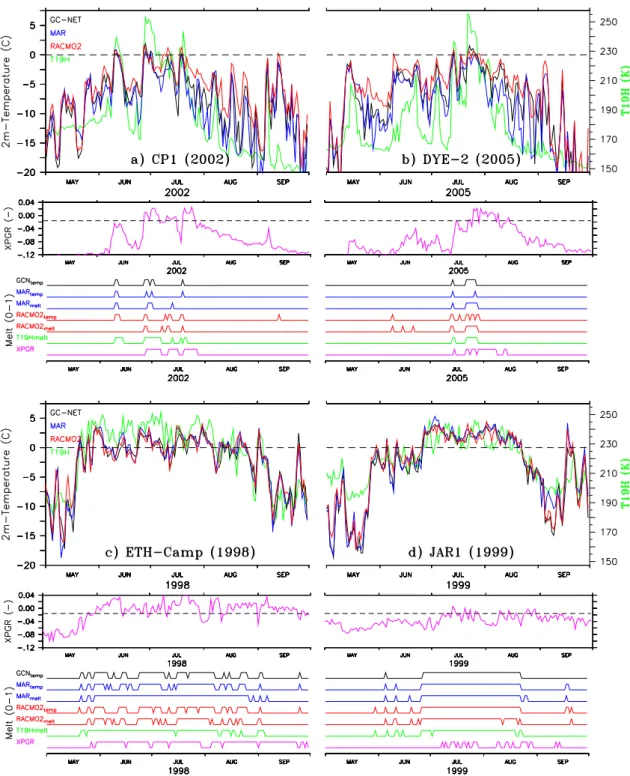
Figure 1 shows time series of near-surface temperature simulated by the two RCMs (MAR and RACMO2) together with GC-Net-measured air temperature for the CP-1, Dye-2, ETH-Camp and JAR1 GC-Net stations for selected years. For each station, the temporal trend of the K-band horizon-tally polarized brightness temperature is also presented. In addition, we also show the temporal trend of the XPGR, to-gether with a binary plot in which melting was derived us-ing different approaches is indicated by the value 1 and no-melting is indicated by the value 0. The comparison between the near-surface temperature simulated by the RCMs and the measured one at GC-Net stations shows that, over the period 1995–2005, the biases in modeled temperature are very low: MAR (respectively RACMO2) underestimates (resp.
over-estimates) the measured near-surface temperature by 0.2◦C (resp. 1.3◦C) (see Table 1).
We use two criteria for detecting the melt events in the RCM modeled time series (a list of the algorithms used to retrieve melt can be found in Table 2). The first one, (RCMtemp), uses a modeled positive daily mean 2 m-temperature as melt threshold and compares favorably with the GC-Net temperature-based time series melt detection (see Table 1). The second approach, (RCMmelt), uses a threshold in modeled daily meltwater production as melt events detection and compares better on average with the T19H-derived melt time series, as we will see in the next sec-tion. The best agreement between the melt/no melt time se-ries using observed daily mean temperature over the 20 GC-NET AWS listed by Steffen and Box (2001) and the melt time series derived from T19H by using Eq. (1) is obtained with T19Hthsd=227.5±2.5 K (see Table 3), with more than 95% of melt events detected. Figure 1 shows melt and tem-perature time series for four GC-Net AWS where consider-able melting is recorded. We have selected in Fig. 1 four summers for four different AWS’s where no gap is present in the data.
Obviously, it would be ideal to compare melt events de-tected with the T19H time series with measurements of snow properties, in particular liquid water content (LWC), because the snowpack response to positive air temperatures is com-plex and melting also depends on other factors, such as albedo, for example. Unfortunately, LWC is not recorded by the GC-Net AWS. Therefore, we use the results from RCMs coupled with a snow model to refine our analysis.
The daily Eq. (1)-derived melt signal has been compared for the period 1979–2009 with corresponding time series simulated by the models and applying different melt detec-tion criteria based on a threshold using
– surface and near-surface temperature,
– internal snowpack temperature,
– LWC in the snowpack,
– presence of bare ice at the surface
(surface snow density higher than 900 kg m−3), – meltwater run-off,
– meltwater production.
Table 1.Mean (over the 1995–2005 summers) percentage of number of melt days at 10 GC-Net AWS’s (where melt is observed) when the RCM and the observations are in agreement, when the RCM fails to detect melt and when RCM detects melt while the observations do not. Two approaches, RCM-temp and RCM-melt (explained in Table 2), are used for detecting melt in the RCM modeled time series. The location of the GC-Net AWS’s is also listed. Finally, the mean modeled daily temperature bias (in◦C) with respect to the GC-net measurements over the 1995–2005 summers is also given.
ID Name Location MAR model RACMO2 model
temp. bias (◦C) MARtemp(%) MARmelt temp. bias RACtemp RACmelt
1 Swiss Camp 69.6◦N, 49.2◦W, 1149 m +0.0±0.3 90-5-5 83-2-15 +0.2±˙0.2 89-6-5 85-9-6 2 CP1 69.9◦N, 47.0◦W, 2022 m −0.1±0.5 97-3-1 95-2-3 +1.9±0.4 96-1-3 94-2-4 3 NASA-U 73.9◦N, 49.5◦W, 2368 m +0.9±1.6 100-0-0 100-0-0 +2.3±1.5 100-0-0 100-0-0 4 GITS 77.1◦N, 61.1◦W, 1887 m −0.6±1.1 100-0-0 99-0-0 +0.8±0.9 99-0-0 100-0-0 5 Humboldt 78.5◦N, 56.8◦W, 1995 m −0.8±0.7 100-0-0 99-0-0 +1.0±0.4 100-0-0 100-0-0 7 Tunu-N 78.0◦N, 34.0◦W, 2020 m −0.2±0.4 100-0-0 100-0-0 +1.6±0.3 99-0-0 100-0-0 8 DYE-2 66.5◦N, 46.3◦W, 2165 m −0.7±0.2 98-2-0 96-2-2 +1.3±0.5 96-1-3 93-1-6 9 JAR1 69.5◦N, 49.7◦W, 962 m +0.6±0.4 90-3-7 82-2-15 +0.5±0.4 89-4-7 87-5-8 10 Saddle 66.0◦N, 44.5◦W, 2559 m −1.2±0.3 99-0-0 99-1-1 +1.4±0.3 99-0-1 98-0-2 12 NASA-E 75.0◦N, 30.0◦W, 2631 m +0.0±0.8 100-0-0 100-0-0 +1.7±0.6 100-0-0 100-0-0
Average −0.2±0.6 97-1-1 96-1-4 +1.3±0.5 97-1-2 96-2-3
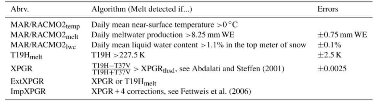
Table 2.Abbreviation of the different techniques discussed in the text to detect the melt. The errors bar range is also listed.
Abrv. Algorithm (Melt detected if...) Errors
MAR/RACMO2temp Daily mean near-surface temperature>0◦C
MAR/RACMO2melt Daily meltwater production>8.25 mm WE ±0.75 mm WE
MAR/RACMO2lwc Daily mean liquid water content>1.1% in the top meter of snow ±0.1%
T19Hmelt T19H>227.5 K ±2.5 K
XPGR T19HT19H−+T37VT37V>XPGRthsd, see Abdalati and Steffen (2001) ±0.0025 ExtXPGR XPGR or T19Hmelt
ImpXPGR XPGR + 4 corrections, see Fettweis et al. (2006)
Table 3.The same as Table 1 but with the T19H-based algorithms for different values of T19Hthsd. The best agreement is written in bold.
ID Name T19Hthsd XPGR
215 K 220 K 225 K 227.5 K 230 K 235 K 240 K
1 Swiss Camp 81-1-18 83-2-15 85-3-12 85-4-10 86-5-9 84-10-5 80-17-3 58-12-30 2 CP1 90-1-10 92-1-8 93-1-6 94-1-5 95-1-4 96-2-2 96-3-1 88-2-10 3 NASA-U 99-0-1 99-0-1 99-0-1 99-0-1 99-0-1 100-0-0 99-0-0 99-0-0 4 GITS 99-0-0 99-0-0 99-0-0 99-0-0 100-0-0 100-0-0 100-0-0 100-0-0 5 Humboldt 99-0-1 99-0-1 99-0-1 99-0-0 99-0-0 99-0-0 99-0-0 100-0-0 7 Tunu-N 100-0-0 100-0-0 100-0-0 100-0-0 100-0-0 100-0-0 100-0-0 100-0-0 8 DYE-2 91-0-8 93-1-7 95-1-5 95-1-4 96-1-3 96-2-2 96-2-2 90-2-8 9 JAR1 78-1-21 82-3-15 83-7-10 81-11-8 77-17-6 67-30-3 56-44-0 49-38-12 10 Saddle 97-0-3 98-0-2 98-0-1 99-0-1 99-0-1 99-1-1 99-1-0 98-1-2 12 NASA-E 100-0-0 100-0-0 100-0-0 100-0-0 100-0-0 100-0-0 100-0-0 100-0-0
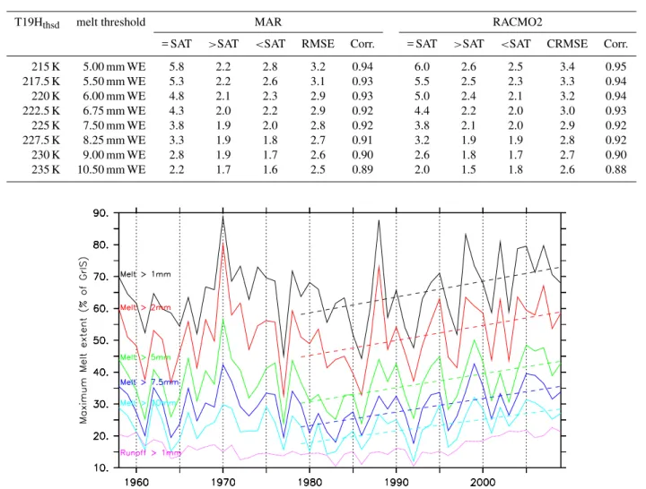
Table 4. Correspondence between Eq. (1)-based and RCM-based melt detection. The mean number of GrIS pixels when both RCM and T19H-based algorithms detect melt (RCM = SAT), when RCM detects melt and not the retrieving algorithms (RCM>SAT) and when RCM
does not detect melt and well the T19H-based algorithms (RCM<SAT) is also listed in percent over the number of GrIS pixels×summer
days. The remaining percent correspond to days where both RCM and T19H-based algorithms do not detect melt. The statistics (i.e. the mean correlation coefficient (Corr.) as well as the mean Root Mean Square Error (RMSE) over 1979–2009) between MAR/RACMO2 and the T19H-based GrIS melt extent time series are also listed.
T19Hthsd melt threshold MAR RACMO2
= SAT >SAT <SAT RMSE Corr. = SAT >SAT <SAT CRMSE Corr.
215 K 5.00 mm WE 5.8 2.2 2.8 3.2 0.94 6.0 2.6 2.5 3.4 0.95
217.5 K 5.50 mm WE 5.3 2.2 2.6 3.1 0.93 5.5 2.5 2.3 3.3 0.94
220 K 6.00 mm WE 4.8 2.1 2.3 2.9 0.93 5.0 2.4 2.1 3.2 0.94
222.5 K 6.75 mm WE 4.3 2.0 2.2 2.9 0.92 4.4 2.2 2.0 3.0 0.93
225 K 7.50 mm WE 3.8 1.9 2.0 2.8 0.92 3.8 2.1 2.0 2.9 0.92
227.5 K 8.25 mm WE 3.3 1.9 1.8 2.7 0.91 3.2 1.9 1.9 2.8 0.92
230 K 9.00 mm WE 2.8 1.9 1.7 2.6 0.90 2.6 1.8 1.7 2.7 0.90
235 K 10.50 mm WE 2.2 1.7 1.6 2.5 0.89 2.0 1.5 1.8 2.6 0.88
Fig. 2. Time series of the maximum melt extent (in percentage of the GrIS area) simulated by MAR for different melt thresholds: daily
meltwater production higher than 1, 2, 5, 7.5 and 10 mm WE and daily runoff higher than 0 mm WE. Finally, the linear trend over 1979–2009 is given by a dashed line.
see hereafter, this suggests that the T19H-based algorithm might not detect melting at the end of the ablation season, when the surface is refreezing but liquid water may still be present in the snowpack or no-melting bare ice may appear on the surface. Unfortunately, no in-situ measurements are available to confirm this hypothesis. We used the same value of daily produced meltwater threshold for both RCMs, which reduced the uncertainty on the relation between T19Hthsdand model-simulated daily meltwater production. Figure 2 shows that the choice of the value (listed in the caption) of the melt threshold used in the RCMs could considerably influence the estimated melt extent area while the linear trends over 1979–
2009 are similar. The comparison between model-simulated and satellite-derived melt extent is discussed in more detail in the next section.
3.2.2 XPGR-based melt detection
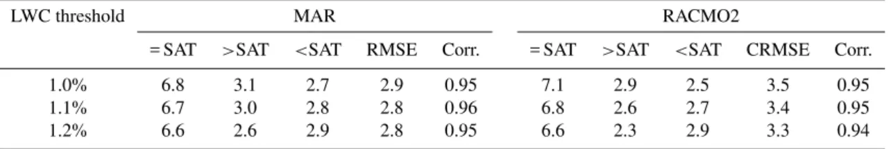
Table 5.The same as Table 4 but for ExtXPGR with T19Hthsd= 227.5 K.
LWC threshold MAR RACMO2
= SAT >SAT <SAT RMSE Corr. = SAT >SAT <SAT CRMSE Corr.
1.0% 6.8 3.1 2.7 2.9 0.95 7.1 2.9 2.5 3.5 0.95
1.1% 6.7 3.0 2.8 2.8 0.96 6.8 2.6 2.7 3.4 0.95
1.2% 6.6 2.6 2.9 2.8 0.95 6.6 2.3 2.9 3.3 0.94
at the ETH-Camp (West-Greenland, 69.6◦N, 49.2◦W) dur-ing the 1990 and 1991 meltdur-ing seasons and correspond ap-proximately to a LWC of 1% by volume in the top meter of snow (Abdalati and Steffen, 1997). Bare ice (melting or not) in the ablation zone is also detected as melting by XPGR. The XPGR threshold varies with the spaceborne passive mi-crowave sensors following Abdalati and Steffen (2001). Ac-cording to Abdalati and Steffen (2001), the XPGR algorithm is sensitive to (sub-)surface melting and to the presence of liquid water in the snowpack when the snow is refreezing at the surface at the end of the summer.
While this approach uses a combination of frequencies compared to T19Hmelt, Fettweis et al. (2005, 2006, 2007) showed that XPGR does not detect melt during rainfall events due to the use of the 37 GHz channel. Consequently, Fettweis et al. (2006) proposed an improved version of XPGR (called ImpXPGR), imposing the continuity of the melt season to remove gaps shorter than three days between two melting days. These gaps are found to be associated with dense clouds, mostly causing liquid precipitation on the ice sheet. However, we have not enough in situ data to affirm that the melt season (presence of liquid meltwater) is contin-uous in time and therefore, this hypothesis needs to be further assessed.
However, knowing that 19 GHz channel is less sensitive to the dense clouds and atmospheric components than the 37 GHz, T19Hmeltcan provide improved performance during these events. That is why we propose here a new approach for improving XPGR by merging the XPGR algorithm of Ab-dalati and Steffen (2001) and T19Hmeltto give:
Melt if XPGR≥XPGRthsd or T19H≥227.5 K
No Melt if XPGR<XPGRthsd and T19H<227.5 K (3) In this case, melting is considered to be occurring if either XPGR or T19H is higher than the corresponding threshold values. We point out that, as in Fettweis et al. (2006), 227.5 K is close to the mean T19H temperature (= 225.3 K) plus half of the standard deviation (= 3.1 K) over 1979–2009 and over all pixels of the whole melt area where XPGR detects melt-ing. This last addition to the XPGR algorithm corresponds to Correction #3 of ImpXPGR (see Fettweis et al., 2006 for more details). This improved version of XPGR will be called hereafter ExtXPGR for Extended XPGR.
In order to compare the XPGR-like algorithms with RCM outputs, we use a modeled LWC higher than 1.1% in the
top meter of snow as melt threshold value above which the model indicates melting in conjunction with the hypothesis of a surface snow density greater than 900 kg m−3for detect-ing bare ice. The value of 1.1% was chosen (instead of 1% as suggested by Abdalati and Steffen, 1997), because it com-pares better with the satellite-derived data set (see Table 5). It is likely that having a better comparison with 1.1% as melt threshold instead of 1.0% is an artifact from the models. Al-though this does not affect the comparison significantly, (the 1.0% value of melt threshold is included in the error bars as inferior boundary), this shows the sensitivity of the models to a difference of 0.1% in the LWC.
4 Melt extent analysis
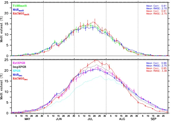
Results from both models and satellites in Fig. 3 indicate that, on the average, the melting season begins in mid-May, culminates in mid-July (when the highest melt extent oc-curs on average), and lasts until the end of September (see Fig. 3), when melting is small or negligible. The average maximum melt extent is between 15 and 20% of the GrIS area (∼1.61×10⁶km2). The melt extent is larger if retrieved by (Ext)XPGR than by T19Hmeltbecause (Ext)XPGR is also sensitive to the presence of LWC into a no-melting snowpack as well as the presence of no-melting bare ice at the surface. The mean correlation between the daily melt extent evolu-tion simulated by the models and that derived from space-borne microwave remote sensing observations is∼0.93 with the mean RMSE being∼3% of the ice sheet surface.
Fig. 3. Mean seasonal cycle (1979–2009) of melt area (in % of GrIS area) simulated by MAR and RACMO2 as well as retrieved from the spaceborne passive microwave data set with the different techniques discussed in the text (see Table 2). The error bars show a posi-tive/negative change of the threshold used to derive the melt extent as listed in Table 2. The statistics (i.e. the mean correlation coefficient as well as the mean Root Mean Square Error over 1979–2009) between MAR (in blue)/RACMO2 (in red) and the T19Hmelt(resp. ExtXPGR) algorithms are also listed.
coming from the reanalysis over the ice sheet. According to Hanna et al. (2009), the impacts of SST changes are for example negligible in MAR over the GrIS. Therefore, the use (or not) of passive microwave data in reanalysis does not significantly influence the comparison of the RCMs with the satellite-derived data.
For the reader’s convenience, comparisons between satel-lite and RCMs for each summer between 1979 and 2009 are reported in the Annex C of the Supplement. We can no-tably observe a large difference between the melt extent es-timated by T19Hmeltand by (Ext)XPGR in September 1982, 1983, 1985, 1987, 1990, 1994, 1999, 2004 and 2006 when T19Hmeltseems, as assumed earlier, not to be sensitive to the presence of non-melting bare ice at the surface or internal liq-uid water into the snow pack, differently from (Ext)XPGR, the latter being in agreement with the results from the mod-els.
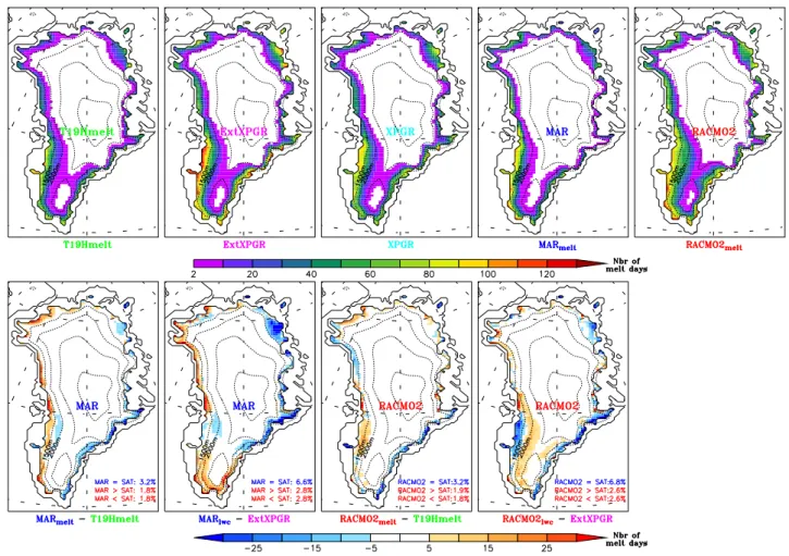
Looking at the number of melting days/summer, it appears that areas with more than 100 melting days/summer in aver-age lie below 70◦N along the ice sheet margin and at the northeast of the ice sheet (Fig. 4). The melt season lasts gen-erally longer in the Southwest with more than four months of melt days detected by ExtXPGR, on average. Over the whole ice sheet, the average difference between the total mean
num-ber of melt days by summer simulated by the models and re-trieved from satellite data with T19Hmelt(resp. ExtXPGR) is 2.5 days (resp. 4.5 days). In 95% of the cases, there is agree-ment among pixel-by-pixel and day-by-day cases between RCMs and satellite-derived melt detected events.
The disagreement between satellite and models can be due to (i) limitations in the algorithms used to derive the melt ex-tent from the microwave data set but also to (ii) biases in the models. The error bars show that using a melt threshold slightly different on both models and on the satellite algo-rithm does not considerably affect the comparison. However, because of the lack of in-situ measurements, it is difficult to clearly identify (i) where and when the satellite estimates are wrong and (ii) when and why the models fail, knowing that the biases may depend on several errors or feedback.
4.1 Some limitations in the remote sensing algorithms
Fig. 4. Top – annual mean total number of melt days derived from the spaceborne passive microwave data and simulated by the RCMs using algorithms described in Table 2. Below – the difference between models and the T19Hmeltand ExtXPGR algorithms. The mean number of GrIS pixels when RCM and the algorithms detect melt (RCM = SAT), when RCM detects melt but the retrieving algorithms do not (RCM>SAT) and when RCM does not detect melt while the algorithms do, (RCM<SAT) is also listed as a percentage of the number
of GrIS pixels×summer days.
The increase in microwave emissivity measured by the ra-diometer when melting occurs may be significantly reduced if a pixel combines both melting and no-melting areas. As considerable melting occurs in these areas, we decided not to remove these pixels from the satellite-models comparison. We only removed pixels near open water (ocean, fjord) as explained in Sect. 2.
The XPGR algorithm detects fewer melt days (about 10%) compared to ExtXPGR (see Fig. 4). This difference is clearly visible along the ice sheet margin where the probability that XPGR is biased by rainfall events or by the presence of clouds with liquid water is high. Figure 1 and Table 3 show that XPGR is less adequate than T19Hmelt or ExtXPGR in detecting melt in the low elevation part of the ablation zone where the probability of rainfall events is the highest and where the probability of melt is the highest, too. Finally, Fig. 3 shows that the differences between XPGR and Ex-tXPGR occur mainly before August and decrease after mid-August when most precipitation falls as snow.
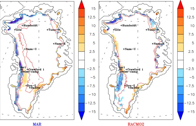
Both RCMs simulate fewer melt days (about 20 days) along the eastern and southeastern mountainous regions of the ice sheet than the microwave-derived estimates (see Fig. 4). Possibly, microwave brightness temperatures could be biased by rock outcrops found in these regions in the Antarctic Peninsula and therefore, the remote sensing algo-rithms may overestimate the occurrence of melt events over this area, as suggested by Torinesi et al. (2003). In ad-dition, this apparent RCM overestimation in respect to the microwave-derived one could also be an artifact induced by the high accumulation rates found in this region, knowing that high accumulation rates induce increases of brightness temperature (Bolzan and Jezek, 2000; Winebrenner et al., 2001). And then, as suggested by the RCMs (see Fig. 5), higher T19Hthsd than 227.5 K should be used in this area to detect the melt events from T19H.
Fig. 5. Value of T19Hthsd(given here as anomaly in K in respect to 227.5 K) which allows the best comparison between the melt extent derived from T19Hmeltand simulated by the RCM (where a daily meltwater production higher than 8.25 mm is used as melt threshold). The GC-Net locations quoted in the text are also shown.
improvement of the comparison between RCMs and satel-lite and more generally, the RCMs agree to suggest that dif-ferences in accumulation rate, snow density,... influence the T19Hthsdvalue. Therefore, using a constant T19Hthsdvalue over each pixel, as assumed in this study, can explain in part the difference between models and satellite. However, it should be noted that biases/discrepancies in both RCMs im-pact also the T19Hthsdvalues computed in Fig. 5. For exam-ple, we can see this impact along the western margin where MAR and RACMO2 suggest different values of T19Hthsd whereas the same daily meltwater production threshold is used in both RCMs for detecting melt events. Unfortunately, most of the GC-net AWSs used to calibrate the T19Hthsd) value are situated in the percolation zone where 227.5 K is the best value for comparing RCM and satellite melt ex-tent. Only one station is located in the ablation zone: JAR1, where the GC-net measurements suggest 220–225 K as the melt threshold (see Table 3) in agreement with the models (see Fig. 5). Therefore, more in-situ observations in the ab-lation zone and along the southeastern mountainous regions are needed to confirm the T19Hthsdvalues suggested by the RCMs.
4.2 Biases in the models
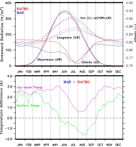
Maximum melt extent area for the melt threshold using the meltwater produced by day (resp. LWC) occurs, on the av-erage, during mid-July. The timing of this maximum is well reproduced by both models (see Fig. 3). However, from May to mid-June (resp. in July), RACMO2 underesti-mates (resp. overestiunderesti-mates) the melt area with respect to both satellite-based melt retrieval algorithms. The largest bias in MAR occurs in July when MAR underestimates the melt area if the meltwater production is used as the melt threshold in the passive microwave data. As we will see, discrepancies in the modeled surface radiation balance most likely explain these disagreements between both RCMs.
Fig. 6. Top – time series of the mean shortwave (solid line), longwave (dotted line), albedo (dashed line on right y-axis) and net radiation (dashed line) averaged over the melting zone of the GrIS (i.e. surface height below 2500 m) and over the period 1979–2009 simulated by MAR (in blue) and by RACMO2 (in red). Below) Time series of the mean difference in surface temperature (resp. the temperature of the top meter of snow) between MAR and RACMO2.
the surface snow albedo decreases earlier in MAR than in RACMO2 at the end of spring and reaches the dry snow albedo earlier as suggested by Torinesi et al. (2003) at the beginning of the winter, because the density of the snow sur-face (which prescribes the albedo in RACMO2) varies more slowly than the surface snow grains morphological charac-teristics (which determine the albedo in MAR) (Lefebre et al., 2003). However, it should be noted that part of differ-ences between the MAR and RACMO2 values of albedo are enhanced by the melt-albedo positive feedback.
Knowing that RACMO2 underestimates the satellite-derived melt extent in May–June unlike MAR, we can sug-gest that at the beginning of the melt season, the snow albedo parametrization used in RACMO2 is not sensitive enough to wet snow conditions compared to the one used in MAR which simulates a lower albedo than RACMO2 during this period (see Fig. 6). In addition to differences in the surface albedo parametrization, the MAR infrared radiative surplus in winter also favors an earlier beginning of the ablation sea-son because the snowpack is warmer in MAR at the end of spring than in RACMO2.
In July, RACMO2 overestimates (note that it is the op-posite for MAR) the melt extent compared to the satellites, likely because the RACMO2 albedo is too low as already suggested in Ettema et al. (2010). The downward longwave underestimation in MAR probably explains the melt extent underestimation in July.
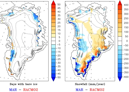
Fig. 7.Left – the mean difference in the number of days (per year) with bare ice at the surface simulated by MAR and by RACMO2. Right – the same but for the annual snowfall in mm WE.
At the end of the melting season (mid-August to Septem-ber), RACMO2 underestimates the melt area only if the LWC is used as melt threshold (Fig. 3). The LWC in RACMO2 is limited to 2% of open pore space, whereas this is 6% in the MAR model. Excess liquid water runs directly off in both models. Therefore, at the end of the melting season, there is still liquid water in the MAR snowpack while most of the meltwater is already refrozen in RACMO2. This could be the reason why RACMO2 underestimates the melt extent in August if LWC is used as melt threshold and also why the MAR snowpack is warmer (refreezing of the retained meltwater prevents initial winter cooling of the snow pack). However, a LWC maximum reaching 6% in MAR could be also too high as we can see after an early (June 1979, 1988) or late (September 1999, 2004) melt event (see the Supple-ment) when MAR overestimates the area where liquid water is present in the snowpack while no more melt is simulated and observed (see T19Hmelt) at the surface.
The patterns of differences between the RCMs and T19Hmeltare quite similar (see Fig. 4). Simulated melt ex-tent is underestimated with respect to T19Hmelt along the southeastern margin and overestimated over the rest of the melt area. The differences are small compared to the dif-ferences with ExtXPGR. The main difference between MAR and RACMO2 occurs along the northwestern coast, where MAR overestimates the melt extent while RACMO2 under-estimates it with respect to T19Hmelt. The differences be-tween the outputs of the two RCMs are further discussed in the following paragraph.
If we use the LWC as the melt threshold, MAR overes-timates the melt extent along the northwestern coast and in South Greenland and underestimates it in West and North Greenland with respect to ExtXPGR. The RACMO2 biases compared to ExtXPGR are very different, with an overes-timation in the North and in the interior of South Green-land. These discrepancies are mainly due to differences in the snow model and in the snowfall pattern, affecting the number of days when bare ice is present on the surface.
1. As discussed earlier, MAR identifies melting areas that are absent in RACMO2 after Mid-August, likely be-cause the maximum LWC in MAR could be 3 times larger that in RACMO2. This also explains why MAR and RACMO2 outputs differ in South Greenland. 2. In addition to the presence of LWC, a pixel is
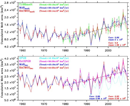
Fig. 8.Time evolution of the annual cumulated GrIS melt area simulated by the RCMs and retrieved from the spaceborne passive microwave data set with the different techniques discussed in the text (see 2). The cumulated melt area is defined as the annual total sum of every daily ice sheet melt area. The linear trend (dashed line) as well as the error bars (see Table 2) are also shown. The uncertainty range of the trend denotes three standard deviations of the trend i.e. a significance of 99%.
also impacts melting by increasing the albedo for a short period after a snowfall event. Differences in snowfall likely explains why RACMO2 underestimates melt ex-tent (compared to T19Hmelt) along the northwestern ice sheet margin.
3. In the North, both modeled precipitation distributions are similar, although MAR simulates fewer bare ice pixels. However, the smallest thickness for a new top layer in the snow model is 2 mm water equivalent (WE) in MAR and 6.5 cm WE in RACMO2. Therefore, RACMO2 needs 6.5 cm WE of fresh snow to create a new layer above bare ice, while a few mm of WE is enough in MAR to change a bare ice (and then melt-ing) pixel to a non-melting pixel. This difference in the minimum layer thickness impacts the results mainly in the dry North where only a few snowfall events occur in summer. This explains also, in addition to the dif-ferences in the surface albedo parametrization, why the surface albedo reaches dry snow values at the end of the ablation season sooner in MAR than in RACMO2.
5 Interannual variability
According to previous studies (Fettweis et al., 2007; Mote, 2007; Tedesco et al., 2008), both microwave-derived and model-simulated melt extent show a significant (99% confidence level) positive trend of melt extent (Fig. 8). Since 1979, the annual cumulated melt extent area (i.e. the annual total sum of every daily ice sheet melt area) has dou-bled. Figure 9 shows that positive trends in melt extent occur everywhere in both the ablation and percolation zones. The slope of the trend in the case of the XPGR-based melt area following Abdalati and Steffen (2001) is not significant (see Fig. 8). This is most likely because rainfall and clouds with liquid water (which perturbs the melt detection by XPGR) also increased in summer over the period 1979–2009 (see Fettweis et al., 2006 and Annex D in the Supplement).
Fig. 9.Linear melt trend (in ablation days yr−1) detected by T19Hmeltand simulated by the models for the period 1979–2009.
regression to cross-calibrate the five sensors is sufficient to apply the same threshold throughout the whole period in Eq. (1), (ii) the modeled melt variability is good and then, (iii) that the RCMs can be used to estimate the melt extent prior to 1979. The RCMs show in Fig. 8 that
1. the cumulated melt extent has been decreasing since the end of the 1950’s to reach its minimum at the beginning of the satellite period,
2. the cumulated melt extent of 1998, 2003, 2005 and 2007 are unprecedented in the last 50 yr,
3. the cumulated melt extent of 2000’s is two times larger than those in the 1970–1980’s,
4. the melting areas during the 1970’s and the 1980’s were comparable,
5. there is a periodicity of 2–3 yr (about 30 months) in the time series, i.e. a summer with a high cumulated melt extent is mostly followed by a summer with less melt. A similar variability is found in the North Atlantic Os-cillation (Nicolay et al., 2008), which is known to influ-ence the summer temperature over the GrIS (Fettweis, 2007).
6 Discussion and conclusion
The results from two RCMs have been compared with mi-crowave brightness temperature-based melt extent estimates
with the objective of studying the evolution of melting over the GrIS since 1958.
We selected two algorithms to retrieve melt extent from the spaceborne passive microwave data set. The first one, using a fixed threshold on the T19H brightness temperature (see Eq. 1), is especially sensitive to the production of surface and sub-surface meltwater by day. The second one, based on the XPGR algorithm from Abdalati and Steffen (1997) (see Eq. 3), detects melt when liquid water is present in the snow pack. The time evolution of melt area over the GrIS through summer and the number of melt days compare very well with the results from both models. The retrieving algorithms as well as the RCMs show a significant (p-value = 0.01) increase of the melt area over the GrIS since 1979. The models show that the recent cumulated melt extents are without precedent in the 50 last years and are two times larger that the ones from the 1980’s.
The close agreement between remote sensing results and model outputs provides robustness to the melt retrieving al-gorithms and melt threshold used. This intercomparison also allowed us to highlight some biases in the models:
1. Differences in response time to surface snow changes in the albedo parametrizations used by RACMO2 explains likely why RACMO2 underestimates the melt extent at the beginning of the melt season and overestimates it in July.
3. The LWC in the RACMO2 snow model is currently lim-ited to 2% (compared to 6% in the MAR model) which prevents melt detection at the end of the ablation season when freezing conditions occur at the surface and there is normally still liquid meltwater in the snow pack. In addition, a maximum LWC value of 6% in MAR likely overestimates the melt extent after high melt events. High quality snow observations at several locations on the ice sheet, helped to select the maximum LWC value in the snow pack.
4. The minimum thickness of a new layer in the RACMO2 snow model is 6.5 cm WE, compared to 2 mm WE in the MAR model. This overestimates in RACMO2 the pix-els with bare ice in the ablation zones where few snow-fall events occur in summer. But in MAR, knowing that it underestimates the melt extent at the north of the ice sheet, the minimum layer thickness threshold should be increased to enhance the agreement with remote sensing data.
5. The comparison with the LWC-sensitive algorithms shows that there are some biases in both simulated pre-cipitation patterns. The winter snowfall accumulation impacts the appearance of bare ice at the surface in sum-mer which is detected as wet by the XPGR-based algo-rithms.
However, part of the discrepancies between satellite and models comes from the microwave data itself which is biased by the tundra or rock pixels nearby the ice sheet or by use of a constant T19H melt threshold over each pixel, whereas the RCMs suggest that snowpack behaviors may significantly influence the T19Hthsdvalue. More in-situ measurements are needed to support these hypothesises.
The close agreement between the RCM results and the microwave-derived melt extent suggests that the RCMs could be run in an assimilation mode, constrained by the space-borne passive microwave data. Indeed, the snowpack prop-erties of the pixels where RCM and satellite disagree could be adjusted. For example, if the RCM has to detect melt in respect to the satellite observations, but does not simu-late it, the snowpack temperature could be increased to reach conditions more favorable to melt while the water mass is conserved. As a future development, we could associate a meltwater threshold as in Table 4 to each brightness temper-ature and assimilate it in the model to improve the meltwater production simulation. This could have significant impact on the modeled meltwater run-off.
Moreover, this study has shown that large uncertainties re-main in the modeled bare ice appearance at the surface while most of the meltwater run-off occurs on this area. There-fore, the MODIS-based albedo could be used for evaluating the bare ice zones in the models and afterwards, for forcing the models in an assimilation mode. Knowing that the GrIS run-off variability is driven to a large part by the bare ice
area variability, this assimilation should help to improve the matching with other satellite data sets (GRACE,...), with the objective of reducing the uncertainties of the SMB model-based estimates.
Supplementary material related to this article is available online at:
http://www.the-cryosphere.net/5/359/2011/ tc-5-359-2011-supplement.pdf.
Acknowledgements. Xavier Fettweis is a postdoctoral researcher of the Belgian National Fund for Scientific Research. Marco Tedesco’s work was supported through the NSF Arctic Natural Sciences grant # 0909388 and the NASA Cryosphere Program.
Edited by: J. L. Bamber
References
Abdalati, W. and Steffen, K.: Snowmelt on the Greenland ice sheet as derived from passive microwave satellite data, J. Climate, 10, 165–175, 1997.
Abdalati, W. and Steffen, K.: Greenland ice sheet melt extent: 1979–1999, J. Geophys. Res., 106, 33983–33988, 2001. Abdalati, W., Steffen, K., Otto, C., and Jezek, K. C.: Comparison
of brightness temperatures from SSMI instruments on the DMSP F8 and FII satellites for Antarctica and the Greenland ice sheet, Int. J. Remote Sens., 16(7), 1223–1229, 1995.
Armstrong, R. L., Knowles, K. W., Brodzik, M. J., and Hardman, M. A.: DMSP SSM/I Pathfinder daily EASE-Grid brightness temperatures, May 1987 to April 2009, Boulder, CO, USA: Na-tional Snow and Ice Data Center, Digital media and CD-ROM, 1994.
Bolzan, J. F. and Jezek, K. C.: Accumulation rate changes in central Greenland from passive microwave data Polar Geography, 1939-0513, 24(2), 98–112, 2000.
Brodzik, M. J. and Armstrong, R. L.: Near-Real-Time DMSP SSM/I-SSMIS Pathfinder Daily EASE-Grid Brightness Temper-atures, June 2009 to September 2009, Boulder, CO USA: Na-tional Snow and Ice Data Center, Digital media, 2008.
Brun, E., David, P., Sudul, M., and Brunot, G.: A numerical model to simulate snowcover stratigraphy for operational avalanche forecasting, J. Glaciol., 38, 13–22, 1992.
Ettema, J., van den Broeke, M. R., van Meijgaard, E., van de Berg, W. J., Bamber, J. L., Box, J. E., and Bales, R. C.: Higher sur-face mass balance of the Greenland ice sheet revealed by high-resolution climate modeling, Geophys. Res. Lett., 36, L12501, doi:10.1029/2009GL038110, 2009.
Ettema, J., van den Broeke, M. R., van Meijgaard, E., van de Berg, W. J., Box, J. E., and Steffen, K.: Climate of the Greenland ice sheet using a high-resolution climate model –Part 1: Evaluation, The Cryosphere, 4, 511–527, doi:10.5194/tc-4-511-2010, 2010. Fettweis, X.: Reconstruction of the 1979–2006 Greenland ice sheet
surface mass balance using the regional climate model MAR, The Cryosphere, 1, 21–40, doi:10.5194/tc-1-21-2007, 2007. Fettweis, X., Gall´ee, H., Lefebre, L., and van Ypersele, J.-P.:
model and comparison with satellite derived data in 1990–1991, Clim. Dynam., 24, 623–640, doi:10.1007/s00382-005-0010-y, 2005.
Fettweis, X., Gall´ee, H., Lefebre, L., and van Ypersele, J.-P.: The 1988–2003 Greenland ice sheet melt extent by passive mi-crowave satellite data and a regional climate model, Clim. Dy-nam., 27(5), 531–541, doi:10.1007/s00382-006-0150-8, 2006. Fettweis, X., van Ypersele, J.-P., Gall´ee, H., Lefebre, F., and
Lefeb-vre, W.: The 1979–2005 Greenland ice sheet melt extent from passive microwave data using an improved version of the melt retrieval XPGR algorithm, Geophys. Res. Lett., 34, L05502, doi:10.1029/2006GL028787, 2007.
Fettweis, X., Hanna, E., Gall´ee, H., Huybrechts, P., and Erpicum, M.: Estimation of the Greenland ice sheet surface mass balance for the 20th and 21st centuries, The Cryosphere, 2, 117–129, doi:10.5194/tc-2-117-2008, 2008.
Fettweis, X., Mabille, G., Erpicum, M., Nicolay, S., and van den Broeke, M.: The 1958–2009 Greenland ice sheet surface melt and the mid-tropospheric atmospheric circulation, Clim. Dy-nam., 36(1), 139–159, doi:10.1007/s00382-010-0772-8, 2011. Gall´ee, H. and Schayes, G.: Development of a three-dimensional
meso-γ primitive equations model, Mon. Weather Rev., 122,
671–685, 1994.
Greuell, W. G. and Konzelmann, T.: Numerical modelling of the energy balance and the englacial temperature of the Greenland Ice Sheet. Calculations for the ETH-Camp location (West Green-land, 1155 m a.s.l.), Global Planet. Change, 9, 91–114, 1994. Joshi, M., Merry, C. J., Jezek, K. C., and Bolzan, J. F.: An edge
detection technique to estimate melt duration, season and melt extent on the Greenland Ice Sheet using Passive Microwave Data, Geophys. Res. Lett., 28(18), 3497–3500, 2001.
Hall, D. K., Williams, R. S., Luthcke, S. B., and Digirolamo, N. E.: Greenland ice sheet surface temperature, melt and mass loss: 2000–2006, J. Glaciol., 54(184), 81–93, 2008.
Hanna, E., Huybrechts, P., Steffen, K., Cappelen, J., Huff, R., Shu-man, C., Irvine-Fynn, T., Wise, S., and Griffiths, M.: Increased runoff from melt from the Greenland Ice Sheet: a response to global warming, J. Climate, 21, 331–341, 2008.
Hanna, E., Cappelen, J., Fettweis, X., Huybrechts, P., Luckman, A., and Ribergaard, M. H.: Hydrologic response of the Greenland ice sheet: the role of oceanographic warming, Hydrol. Process., 23 (1), 7–30, 2009.
Knowles, K., Njoku, E., Armstrong, R., and Brodzik, M. J.: Nimbus-7 SMMR Pathfinder Daily EASE-Grid Brightness Tem-peratures [CD-ROM], Natl. Snow and Ice Data Cent., Boulder, Colo, 2002.
Lefebre, F., Gall´ee, H., van Ypersele, J., and Greuell, W.: Mod-eling of snow and ice melt at ETH-camp (west Greenland): a study of surface albedo, J. Geophys. Res., 108(D8), 4231, doi:10.1029/2001JD001160, 2003.
Liu, H., Wang, L., and Jezek, K. C.: Spatiotemporal variations of snowmelt in Antarctica derived from satellite scanning multi-channel microwave radiometer and Special Sensor Microwave Imager data (1978–2004), J. Geophys. Res., 111, F01003, doi:10.1029/2005JF000318, 2006.
Luthcke, S. B., Zwally, H. J., Abdalati, W., Rowlands, D. D., Ray, R. D., Nerem, R. S., Lemoine, F. G., McCarthy, J. J., and Chinn, D. S.: Recent Greenland Ice Mass Loss by Drainage System from Satellite Gravity Observations, Science, 314(5803), 1286,
doi:10.1126/science.1130776, 2006
Mote, T. L.: Greenland surface melt trends 1973–2007: Evidence of a large increase in 2007, Geophys. Res. Lett., 34, L22507, doi:10.1029/2007GL031976, 2007.
Nicolay, S., Mabille, G., Fettweis, X., and Erpicum, M.: 30 and 43 months period cycles found in air temperature time series us-ing the Morlet wavelet method, Clim. Dynam., 33(7–8), 1117– 1129, doi:10.1007/s00382-008-0484-5, 2008.
Picard, G. and Fily, M.: Surface melting observations in Antarc-tica by microwave radiometers: correcting 26-year long time se-ries from changes in acquisition hours, Remote Sens. Environ., 104(3), 325–336, 2006.
Steffen, K. and Box, J. E.: Surface climatology of the Greenland ice sheet: Greenland Climate Network 1995–1999, J. Geophys. Res., 106(D24), 33951–33964, 2001.
Ulaby, F. and Stiles, W.: The active and passive microwave response to snow parameters. 2: water equivalent of dry snow, J. Geophys. Res., 85, 1045–1049, 1980.
Tedesco, M.: Snowmelt detection over the Greenland ice sheet from SSM/I brightness temperature daily variations, Geophys. Res. Lett., 34, L02504, doi:10.1029/2006GL028466, 2007.
Tedesco, M.: Assessment and development of snowmelt retrieval algorithms over Antarctica from K-band spaceborne brightness temperature (1979–2009), Remote Sens. Environ., 113(5), 979– 997, 2009.
Tedesco, M., Serreze, M., and Fettweis, X.: Diagnosing the extreme surface melt event over southwestern Greenland in 2007, The Cryosphere, 2, 159–166, doi:10.5194/tc-2-159-2008, 2008. Tedesco, M., Fettweis, X., van den Broeke, M., van de Wal, R.,
Smeets, P., van de Berg, W. J., Serreze, M., and Box, J.: The role of albedo and accumulation in the 2010 melting record in Greenland, Environ. Res. Lett., 6(1), 014005, doi:10.1088/1748-9326/6/1/014005, 2011.
Torinesi, O., Fily, M., and Genthon, C.: Variability and trends of the summer melt period of Antarctic ice margin since 1980 from microwave sensors, J. Climate, 16, 1047–1060, 2003.
Van den Broeke, M. R., Bamber, J., Ettema, J., Rignot, E., Schrama, E., van de Berg, W. J., van Meijgaard, E., Velicogna, I., and Wouters, B.: Partitioning recent Greenland mass loss, Science, 326, 984–986, 2009.
Wake, L. M., Huybrechts, P., Box, J. E., Hanna, E., Janssens, I., and Milne, G. A.: Surface mass-balance changes of the Greenland ice sheet since 1866, Ann. Glaciol., 50(50), 178–184, 2009. Winebrenner, D. P., Arthern, R. J., and Shuman, C. A.:
Map-ping Greenland accumulation rates using observations of ther-mal emission at 4.5-cm wavelength, J. Geophys. Res., 106(D24), 33919–33934, 2001.
Wouters, B., Chambers, D., and Schrama, E. J. O.: GRACE ob-serves small-scale mass loss in Greenland, Geophys. Res. Lett., 35, L20501, doi:10.1029/2008GL034816, 2008.
Zwally, H. J. and Fiegles, S.: Extent and duration of Antarctic sur-face melting, J. Glaciol., 40(136), 463–476, 1994.