Brazilian Journal of Physics, vol. 37, no. 1, March, 2007 63
X (3872) in QCD Sum Rules
R. D. Matheus
Instituto de F´ısica, Universidade de S˜ao Paulo, C.P. 66318, 05315-970, S˜ao Paulo, SP, Brazil
Received on 29 September, 2006
QCD spectral sum rules is used to test the nature of the mesonX(3872), assumed to be an exotic four-quark(ccq¯ q¯)state withJPC=1++. For definiteness, the current proposed recently by Maiani et al [1] is used, at leading order inαs, considering the contributions of higher dimension condensates. The valueMX = (3.94±0.11)GeV is found which is compatible, within the errors, with the experimental candidate X(3872). The uncertainties of our estimates are mainly due to the one from thecquark mass.
Keywords: QCD sum rules; Tetraquarks; Axial vector mesons
I. INTRODUCTION
In august 2003, there’s been a report by BELLE[2] of a nar-row resonance inB+→X(3872)K+→J/ψ π+π−K+decays. It has been soon after confirmed by D0 [3], CDF II [4] and BABAR [5]. The collective data from these experiments give an averaged mass ofmX=3871,9±0,5 MeV [6]. The width
has been stablished by BELLE at a upper limit of 2,3 MeV at 90% confidence level and the most probable quantum num-bers are:JPC=1++[6].
BELLE has also found the resonance in the channel: X(3872)→J/ψ π+π−π0 . The relative strength of this
de-cay mode is given by[7]:
Br¡
X→π+π−π0J/ψ¢
Br(X→π+π−J/ψ) =1.0±0.4±0.3 (1)
This strong isospin violation makes it difficult to understand the X as a charmoniun. Besides, the charmoniun spectrum state with correct quantum numbers,χ1′(3925), has both the mass and the decay width (≈16 MeV) too high to be grace-fully identified with the observed resonance[6].
The anomalous nature of the X has led to many specula-tions: tetraquark [1, 8], cusp [9], hybrid [10], or glueball [11]. Another explanation is that theX(3872)is aDD¯∗bound state [12–16], as predicted before its discovery.
In this work the QCD spectral sum rules (the Borel/Laplace Sum Rules (SR) [17–19] and Finite Energy Sum Rules (FESR) [19–21]) will be used to study the two-point func-tions of the axial vector meson, X(3872), assumed to be a four-quark state. In previous calculations, the Sum Rule (SR) approach was used to study the light scalar mesons [22–25] and theD+sJ(2317)meson [26, 27], considered as four-quark states and a good agreement with the experimental masses was obtained. However, the tests were not decisive as the usual quark–antiquark assignments also provide predictions consis-tent with data and more importantly with chiral symmetry ex-pectations [19, 23, 28, 29]. In the four-quark scenario, scalar mesons can be considered as S-wave bound states of diquark-antidiquark pairs, where the diquark was taken to be a spin zero color anti-triplet. Ref. [1] will be followed here, and theX(3872)will be considered as aJPC=1++state with the
symmetric spin distribution: [cq]S=1[c¯q¯]S=0+ [cq]S=0[c¯q¯]S=1.
Therefore, the corresponding lowest-dimension interpolating operator for describingXqis given by:
jµ=
iεabcεdec
√ 2 [(q
T
aCγ5cb)(q¯dγµCc¯Te) + (qTaCγµcb)(q¯dγ5Cc¯Te)],
(2) wherea,b,c, ...are color indices,Cis the charge conjugation matrix andqdenotes auordquark.
II. THE QCD EXPRESSION OF THE TWO-POINT
CORRELATOR
The SR are constructed from the two-point correlation function
Πµν(q) = i
Z
d4x eiq.xh0|T[jµ(x)jν†(0)]|0i=
= −Π1(q2)(gµν−
qµqν
q2 ) +Π0(q 2)qµqν
q2 . (3)
Since the axial vector current is not conserved, the two func-tions,Π1 andΠ0, appearing in Eq. (3) are independent and
have respectively the quantum numbers of the spin 1 and 0 mesons.
The fundamental assumption of the sum rules approach is the principle of duality. Specifically, we assume that there is an interval over which the correlation function may be equiv-alently described at both the quark and the hadron levels. Therefore, on one hand, we calculate the correlation func-tion at the quark level in terms of quark and gluon fields. On the other hand, the correlation function is calculated at the hadronic level introducing hadron characteristics such as masses and coupling constants. At the quark level, the com-plex structure of the QCD vacuum leads us to employ the Wil-son’s operator product expansion (OPE). The calculation of the phenomenological side proceeds by inserting intermediate states for the mesonX. Parametrizing the coupling of the ax-ial vector meson 1++,X, to the current, jµ, in Eq. (2) in terms
of the meson decay constant fX as:
h0|jµ|Xi=
√
2fXMX4εµ, (4)
the phenomenological side of Eq. (3) can be written as
Πphenµν (q2) = 2f
2 XM8X
M2 X−q2
µ −gµν+
qµqν
M2 X
¶
64 R. D. Matheus
where the Lorentz structure projects out the 1++ state. The dots denote higher axial-vector resonance contributions that will be parametrized, as usual, through the introduction of a continuum threshold parameters0.
The OPE side will be evaluated at leading order inαsand
the contributions of condensates will be considered up to di-mension five.
The correlation function,Π1, in the OPE side can be written
as a dispersion relation:
ΠOPE 1 (q2) =
Z ∞
4m2 c
ds ρ(s)
s−q2, (6)
where the spectral density is given by the imaginary part of the correlation function: πρ(s) =Im[ΠOPE
1 (s)]. After
mak-ing an inverse-Laplace (or Borel) transform of both sides, and transferring the continuum contribution to the OPE side, the sum rule for the axial vector meson X up to dimension-five condensates can be written as:
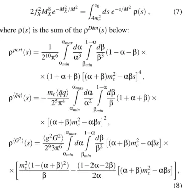
2fX2M8Xe−M2X/M2= Z s0
4m2 c
ds e−s/M2ρ(s), (7) whereρ(s)is the sum of theρDim(s)below:
ρpert(s) = 1
210π6 αmax Z
αmin
dα α3
1−α
Z
βmin
dβ
β3(1−α−β)×
×(1+α+β)£
(α+β)m2c−αβs¤4 ,
ρhqq¯i(s) =−mchqq¯ i 25π4
αmax Z
αmin
dα α2
1−α
Z
βmin
dβ
β (1+α+β)×
×£
(α+β)m2c−αβs¤2 ,
ρhG2i(s) =hg
2G2i
293π6 αmax
Z
αmin
dα
1−α
Z
βmin
dβ β2
£
(α+β)m2c−αβs¤ ×
× ·
m2c(1−(α+β)2)
β −
(1−2α−2β)
2α
£
(α+β)m2c−αβs¤ ¸
,
(8) where the integration limits are given by αmin =
(1−p1−4m2
c/s)/2, αmax = (1+
p 1−4m2
c/s)/2 and
(βmin=αm2c)/(sα−m2c). The dominant contributions from
the dimension-five condensates have also been included :
ρmix(s) =mchqgσ¯ .Gqi
26π4
αmax Z
αmin
dα
·
−α2(m2c−α(1−α)s) +
+
1−α
Z
βmin
dβ£
(α+β)m2c−αβs¤ µ
1 α+
α+β β2
¶ ¸ , (9)
III. LSR PREDICTIONS OFMX
In order to extract the massMXwithout worrying about the
value of the decay constantfX, one must take the derivative of
Eq. (7) with respect to 1/M2, divide the result by Eq. (7) and obtain:
MX2=
Rs0
4m2 cds e
−s/M2 sρ(s)
Rs0
4m2 cds e
−s/M2
ρ(s) . (10)
In the numerical analysis of the sum rules, the values used for the quark masses and condensates are (see e.g. [19, 30–32]):mc= (1.23±0.05)GeV,mu=2.3 MeV ,md=
6.4 MeV, mq= (mu+md)/2=4.3 MeV, hqq¯ i= −(0.23±
0.03)3GeV3,
hqgσ¯ .Gqi=m20hqq¯ i withm20=0.8 GeV2 and hg2G2i=0.88 GeV4. The sum rules were evaluated in the range 1.6≤M2≤2.8 for three values ofs
0: s10/2=4.1 GeV,
s10/2=4.3 GeV ands10/2=4.5 GeV.
Comparing the relative contribution of each term in Eqs. (8) and (9), to the right hand side of Eq. (7) there is a quite good OPE convergence forM2>1.9 GeV2. This analysis allows
us to determine the lower limit constraint forM2in the sum rules window [33].
The upper limit constraint forM2is determined by impos-ing that the QCD continuum contribution should be smaller than the pole contribution. The maximum value of M2 for which this constraint is satisfied depends on the value ofs0.
The comparison between pole and continuum contributions givesM2<3.0 fors10/2=4.5 GeV,M2<2.6 fors10/2=4.3 GeV andM2<2.3 GeV2fors10/2=4.1 GeV.
Figure 1 shows theX meson mass obtained from Eq. (10), in the relevant sum rules window, with the upper and lower validity limits indicated. From Fig. 1 we see that the results are reasonably stable as a function ofM2. In the numerical analysis the range ofM2values from 2.1 GeV2until the one allowed by the sum rule window criteria shall then be consid-ered for each value ofs0.
Varying the QCD parameters inside the limits shown before and taking into account the range of values forM2ands0we
get:
MX= (3.94±0.17)GeV (11)
The error is due to the combined effect ofM2,s0,hqq¯ i, and
mc(mchaving the greatest effect).
IV. FESR PREDICTION FORMX
As an alternative, one can use the FESR, which can be ob-tained from Eq. (7) by taking the limit 1/M2→0 and equating the same power in 1/M2in the two sides of the sum rules to
getnequations: 2fX2MX8MX2n=
Z s0
4m2 c
ds snρ(s), n=0,1,2... (12) Finally, dividing two subsequent equations (withnandn+1) one can obtain the massMXfor any chosen value ofn(which,
formally, is expected to be the same for anyn):
MX2=
Rs0
4m2 c
ds sn+1ρ(s)
Rs0
4m2 cds s
Brazilian Journal of Physics, vol. 37, no. 1, March, 2007 65
2.0 2.2 2.4 2.6 2.8 3.0
3.7 3.8 3.9 4.0 4.1 4.2 4.3
s01/2 = 4.1 GeV s01/2 = 4.3 GeV s01/2 = 4.5 GeV
mX
(
G
e
V
)
M2 (GeV2)
FIG. 1: TheXmeson mass as a function of the sum rule parameter (M2) for different values of the continuum threshold:s10/2=4.5 GeV (solid line),s10/2=4.3 GeV (dashed line) ands10/2=4.1 GeV (dot-ted line). The arrows indicate the region allowed for the sum rules: the lower limit (cut below 2.0 GeV2) is given by OPE convergence requirement and the upper limit by the dominance of the QCD pole contribution.
In contrast to the previous method, the FESR have the ad-vantage of giving correlations between the mass and the con-tinuum thresholds0, which can be used to avoid
inconsisten-cies in the determination of these parameters. Ideally, one looks at a minimum in the functionMX(s0), which would
pro-vide a good criteria for fixing boths0andMX. The results for
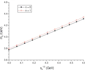
different values ofnare very similar, therefore, in Fig. 2, only the results forn=0 andn=1 are shown. One can see in Fig. 2 that there is no stability ins0, which presumably indicates the
important role of the QCD continuum in the analysis. The FESR results agree with LSR ones only for a small value ofs0: s10/2≈4.2 GeV, but since no stability was found
we consider the LSR to be more reliable in this case.
V. CONCLUSIONS
We have presented a QCD spectral sum rules analysis of the two-point function of theX(3872)meson considered as a
four quark state. We find that the sum rules result in Eq. (11) is compatible with experimental data. An improvement of this result needs an accurate determination ofmc.
Once the mass of theX(3872)is understood, it remains to explain why it is so narrow. There are presumably many mul-tiquark states, but most of them are very broad and cannot be singled out from the continuum. In a recent study [34], based on the same interpolating field as the one used here, it was shown that, in order to explain the small width of theX(3872), one has to choose a particular set of diagrams contributing to its decay. However, it will be desirable if this investigation can
4.0 4.1 4.2 4.3 4.4 4.5 4.6
3.6 3.8 4.0 4.2 4.4 4.6
n = 0 n = 1
mX
(
G
e
V
)
s01/2 (GeV)
FIG. 2: The FESR results in Eq. (13) forMX as a function ofs0for
n=0 andn=1.
be checked from alternative approaches, like e.g. lattice cal-culations. If confirmed, this method can be straightforwardly repeated to a variety of currents for understanding the width and the internal structure of theX(3872).
Acknowledgments
The author acknowledges M. Nielsen, S. Narison and J.-M. Richard for fruitful discussions. This work has been supported by FAPESP.
[1] L. Maiani, F. Piccinini, A.D. Polosa, and V. Riquer, Phys. Rev. D71, 014028 (2005).
[2] S.-L. Choi et al. [Belle Collaboration], Phys. Rev. Lett.91, 262001 (2003).
[3] V. M. Abazov et al. [D0 Collaboration], Phys. Rev. Lett.93, 162002 (2004).
[4] D. Acosta et al. [CDF II Collaboration], Phys. Rev. Lett.93, (2004) 072001.
[5] B. Aubert et al. [BABARCollaboration], Phys. Rev. D 71, 071103 (2005).
[6] Eric S. Swanson, Phys. Rept.429, 243 (2006).
[7] K. Abe et al., “Evidence for X(3872) → gamma J/psi and the sub-threshold decay X(3872) → omega J/psi”, [hep-ex/0505037].
66 R. D. Matheus
[9] D. Bugg, Phys. Lett. B598, 8 (2004). [10] B.-A. Li, Phys. Lett. B605, 306 (2005). [11] K. K. Seth, Phys. Lett. B612, 1 (2005). [12] N. T¨ornqvist, [hep-ph/0308277].
[13] F. E. Close and P. Page, Phys. Lett. B578, 119 (2004). [14] C.Y. Wong, Phys. Rev. C69, 055202 (2004).
[15] S. Pakvasa and M. Suzuki, Phys. Lett. B579, 67 (2004). [16] E. S. Swanson, Phys. Lett. B588, 189 (2004); Phys. Lett. B
598, 197 (2004); Phys. Rept.429, 243 (2006).
[17] M.A. Shifman, A.I. Vainshtein, and V.I. Zakharov, Nucl. Phys. B147, 385 (1979).
[18] L.J. Reinders, H. Rubinstein, and S. Yazaki, Phys. Rept.127, 1 (1985).
[19] S. Narison,QCD as a theory of hadrons, Cambridge Monogr. Part. Phys. Nucl. Phys. Cosmol. 17, (2002) 1-778 [hep-h/0205006]; QCD spectral sum rules, World Sci. Lect. Notes Phys.26, 1-527 (1989).
[20] R. A. Bertlmann, C. A. Dominguez, G. Launer, and E. de Rafa¨el, Nucl. Phys. B 250, 61 (1985); R.A. Bertlmann, G. Launer, and E. de Rafael, Z. Phys. C39, 231 (1988).
[21] K. Chetyrkin, N.V. Krasnikov, and A.N. Tavkhelidze, Phys. Lett. B 76, 83 (1978); N.V. Krasnikov, A.A. Pivovarov, and A.N. Tavkhelidze, Z. Phys. C19, 301 (1983).
[22] J. Latorre and P. Pascual, J. Phys. G11, L231 (1985). [23] S. Narison, Phys. Lett. B175, 88 (1986).
[24] T. V. Brito, F. S. Navarra, M. Nielsen, and M. E. Bracco, Phys. Lett. B608, 69 (2005).
[25] H-J. Lee and N.I. Kochelev, Phys. Lett. B642, 358 (2006).
[26] M. E. Bracco, A. Lozea, R. D. Matheus, F. S. Navarra, and M. Nielsen, Phys. Lett. B624, 217 (2005).
[27] H.-Y. Cheng, W.S. Hou, Phys. Lett. B566, 193 (2003); A. Datta, P. J. O’Donnell, Phys. Lett. B572, 164 (2003). P. Colan-gelo, F. De Fazio, R. Ferrandes, Mod. Phys. Lett. A19, 2083 (2004); A. Hayashigaki, K. Terasaki, hep-ph/0411285; D. Be-cirevic, S. Fajfer, and S. Prelovsek, Phys. Lett. B 599, 55 (2004); Z.-G. Wang, Shao-Long Wan, hep-ph/0602080; J.P. Pfannmoeller , hep-ph/0608213
[28] S. Narison , hep-ph/0512256; S. Narison, Phys. Lett. B605, 319 (2005); S. Narison, Phys. Lett. B210, 238 (1988). [29] W.A. Bardeenet al., Phys. Rev. D68, 054024 (2003); S.
God-frey, Phys. Lett. B568, 254 (2003); M. Haradaet al., Phys. Rev. D70, 074002 (2004); Y.B. Daiet al.Phys. Rev. D68, 114011 (2003).
[30] S. Narison, Nucl. Phys. Proc. Suppl.86, 242 (2000); S. Nar-ison, hep-ph/0202200; S. NarNar-ison, Phys. Rev. D74, 034013 (2006); S. Narison, Phys. Lett. B341, 73 (1994); H.G. Dosch and S. Narison, Phys. Lett. B417, 173 (1998); S. Narison, Phys. Lett. B216, 191 (1989).
[31] S. Narison, Phys. Lett. B466, 345 (1999).
[32] S. Narison, Phys. Lett. B361, 121 (1995); S. Narison, Phys. Lett. B387, 162 (1996). S. Narison, Phys. Lett. B624, 223 (2005).
[33] R. D. Matheus, S. Narison, M. Nielsen, and J. M. Richard, Phys. Rev. D75, 014005 (2007).