Brazilian Journal of Physics, vol. 37, no. 1, March, 2007 37
Numerical Simulation of Ginzburg-Landau-Langevin Equations
N. C. Cassol-Seewald and G. Krein
Instituto de F´ısica Te´orica, Universidade Estadual Paulista, Rua Pamplona 145, 01405-900 S ˜ao Paulo, SP, Brazil
Received on 29 September, 2006
This work is concerned with non-equilibrium phenomena, with focus on the numerical simulation of the relaxation of non-conserved order parameters described by stochastic kinetic equations known as Ginzburg-Landau-Langevin (GLL) equations. We propose methods for solving numerically these type of equations, with additive and multiplicative noises. Illustrative applications of the methods are presented for different GLL equations, with emphasis on equations incorporating memory effects.
Keywords: Mon-equilibrium phenomena; Numerical simulations; Stochastic kinetic equations
I. INTRODUCTION AND MOTIVATION
There are many natural phenomena that occur out of ther-modynamic equilibrium and the study of dynamical phase transitions, in particular, is of interest in diverse branches of physics [1]. Among the different aspects of the subject, the understanding of the relaxation of an order parameter is of particular importance. This topic is related to the fundamen-tal question of how a macroscopic irreversible phenomenon like a phase transition arises from a given microscopic re-versible dynamics. Answering this question is a very difficult task. In most cases one has to use phenomenological dynam-ical equations that contain dissipation and fluctuation terms, known as stochastic kinetic equations. Only in rare situations one can derive such an equation starting with a microscopic model. In general, some sort of coarse graining technique has to be used, in which short wavelengths related to micro-scopic degrees freedom are integrated out in a deterministic equation [2]. This results necessarily in stochastic equations of motion known generically as Ginzburg-Landau-Langevin (GLL) equations.
The traditional GLL equation with additive noise is given by [1]
∂φ(x,t) ∂t =−Γ
δF[φ]
δφ +ξ(x,t) (1) whereΓis an Onsager coefficient,ξis a noise term andF[φ]is the Ginzburg-Landau Hamiltonian. In general,F[φ]is given in terms of a potentialU(φ)as
F[φ] =
d3x
1 2γ(∇φ)
2+U(φ)
(2)
Eq. (1) is a reaction-diffusion type of equation – in the ab-sence ofU(φ)Eq. (1) is precisely the diffusion equation. On general grounds, it is clear that the diffusion equation violates causality – this is also true for Eq. (1). This is so because dif-fusion processes proceed through a collective motion of mat-ter dominated by microscopic scatmat-tering events of infinitely high frequency. In real systems, however, scattering events proceed through finite time intervals and therefore transport memory effects in some circumstances must be taken into ac-count. This is the case for systems in which the time scales of phase conversion are comparable to the microscopic time
scales. One example of a system in which the phase conver-sion is very rapid is the matter formed in high-energy heavy-ion collisheavy-ions.
Memory effects can be introduced phenomenologically in the GLL equation via a memory functionW(t−t′)
∂φ(t) ∂t =
t
0
dt′W(t−t′)
−ΓδF[φ(t′)] δφ(t′) +ξ(t
′) (3)
where we have indicated only the time dependence in the field and noise variables. Now, when the memory function is given by an exponential function of the form
W(t−t′) = 1 αe
−(t−t′)/α
(4)
one can easily show that Eq. (3) can be rewritten as
τ∂ 2φ(x,t)
∂t2 −γ∇
2φ(x,t) + η∂φ(x,t) ∂t +U
′(φ) =
0 (5)
where we have definedU′=U′−ξ, andτ=α/Γandη=1/Γ. The introduction of memory into the GLL equation brings in the second-order time derivative. Such a second-order time derivative appears naturally in a relativistic quantum field the-ory of a scalar field. In particular, an effective GLL equation can be obtained by taking into account quantum corrections up to order2and second order in the coupling constant, whose general form is given by (in the high-temperature limit) [3]
φ(x,t) + η φ2(x,t)∂φ(x,t) ∂t
+ U′[φ,T] =φ(x,t)ξ(x,t) (6) where=∂2/∂t2−∇2, andηis the dissipation coefficient associated with the multiplicative noise fieldξgiven by
η= 96 πT ln
T mT
(7)
andmT is the temperature-dependent mass parameter of the
38 N. C. Cassol-Seewald and G. Krein
The aim of the present paper is to discuss methods for solv-ing numerically the above equations. Specifically we use two discretization procedures for the spatial coordinates, finite dif-ferences and Fourier collocation. For the discretization of the time variable, we use finite differences and leap frog methods. In a separate publication [4] we have performed a numerical analysis for the equations without noise, showing the exis-tence, stability and convergence of the methods for the equa-tions with memory. Here we present results of simulaequa-tions of the GLL equations with additive and multiplicative noises using the methods developed in Ref. [4].
II. NUMERICAL METHODS - ADDITIVE AND MULTIPLICATIVE NOISE
We divide time in n steps, t =n∆t, with n=0,1,2,···. Next, we insert the system in a cubic lattice, whereh=L/N is the lattice spacing and N is the number of lattice sites in each spatial direction, so that the spatial coordinates(x,y,z) are given by
(x,y,z) = (ih,jh,kh) i,j,k = 0,1,2, ....N−1 (8) With this, the fieldφ(x,y,z,t)which originally is a continuous quantity becomes discrete and we represent it asφn
i jk. We treat
the spatial variables using a Fast Fourier Transform method, so that the field is given by
φni jk= N−1
∑
rsp=0anrspErsp(i jk) (9)
with
Ersp(i jk) =exp
i2π Nhxr+i
2π Nhys+i
2π Nhzp
(10)
We use two different approximation schemes to handle the Laplacian term, afinite difference method(FDM) andFourier collocation method (FCM). In FDM we write the Laplacian term by using finite differences for the spatial derivatives, which leads to
∇2φn i jk =
N−1
∑
rsp=0λrspanrspErsp(i jk) (11)
with
λrsp=
1 h2
−6 + 2 cos
2π
Nr
+2 cos
2π
Ns
+ 2 cos
2π
N p
(12)
In the FCM, on the other hand, one simply differentiate the exponential terms in Eq. (10) which leads to a different ex-pression forλrsp, namely
λrsp=
2π Nh
2
r2+s2+p2 (13)
In addition, we define the Fourier transform forU′=U′−ξ as
Uni jk≡Ui jk′n−ξni jk= N−1
∑
rsp=0bnrspErsp(i jk) (14)
With respect to the discretization of the time derivatives, we use two approximation methods,finite differencesandleap frog. In the first method, one has
∂φn i jk
∂t =
N−1
∑
rspan+rsp1−anrsp
∆t Ersp(i jk) ∂2φn
i jk
∂t2 =
N−1
∑
rspan+rsp1−2anrsp+anrsp−1
(∆t)2 Ersp(i jk) (15) In order to simplify presentation, we use an abbreviated nota-tionk={r,s,p}. Therefore, using a semi-implicit method in which the Laplacian term is treated at timen, one obtains the following iteration scheme for the Fourier components of the field
ank=(2τ+η∆t)a n−1
k −τan−
2
rsp −bnk−1(∆t)
2
τ−γλk(∆t)2+η∆t
(16)
where λk is either given by Eq. (12) for the FDM, or by
Eq. (13) for the FCM.
The leap frog algorithm is defined by the iteration scheme
˙
an+k 1/2 = [1−1/2(η∆t)]a˙ n−1/2
k + [λkank−bnk]∆t
1+1/2(η∆t)
akn+1 = ank+a˙n+k 1/2∆t (17) withλkagain given either by Eq. (12) or Eq. (13) as above.
For the case of Eq. (6), one has multiplicative noise. We deal with this in the following way. Initially we lump together in a single function the derivative of the potential and the noise term and define its Fourier transform as
Uni jk≡U′i jkn −φn
i jkξni jk=
∑
kdknEk(i jk) (18)
We also define the Fourier transform of the nonlinear dissipa-tive term as
φ2∂φ ∂t →
φni jk2φ
n i jk−φ
n−1
i jk
∆t =
∑
k cn
kEk(i jk) (19)
With this, the iteration scheme when treating the time deriva-tives with a finite difference scheme is given by the equation
ank=2a n−1
k −a
n−2
k −
ηcnk−1+dkn−1(∆t2) 1−λk(∆t)2
(20)
When treating the time derivatives with the leap frog algo-rithm, one has
˙
an+k 1/2 = a˙nk−1/2+ (λkank−bnk−ηcnk)∆t
Brazilian Journal of Physics, vol. 37, no. 1, March, 2007 39
III. RESULTS OF NUMERICAL SIMULATIONS
In Ref. [4] we have shown that for the one-dimensional case the equations without noise, the methods discussed above are very stable and converge very well with respect to different lattice spacings and time steps. Here we present new results of numerical simulations for the three-dimensional case without and with noise [5]. All results refer to a double-well potential of the form
U(φ) =−1
2φ 2+1
4φ
4 (22)
We concentrate here on the time dependence of the volume average of the order parameter, defined as
φ(x,y,z,t)= 1
N3
∑
i jk
φi jkn (23)
whereφi jkn is the average over a large numberNs of
indepen-dent noise realizations,
φi jkn = 1
Ns Ns
∑
s=1φn
i jk (24)
The equilibrium value (n→∞) of this quantity,φi jk, gives the classical average
φi jk=
[Dφ]φi jke−βF[φ]
[Dφ]e−βF[φ] (25)
As for the one-dimensional case [4], we found that it is pos-sible to obtain stable, converging solutions for the noiseless three dimensional equations for time steps∆t≤0.1 and lat-tice spacingsh=L/N≤1. Once ∆t≤0.1 andh≤1, the results are independent of the lattice spacing. In the top panel of Fig. 1 we plot results for the noncausal equation (τ=0), and in the bottom panel we show the corresponding results for the causal equation (τ=0). The results in this figure are for an initial condition of the form
φ0(i,j,k) =0.01+0.005(2∗ran−1) (26) whereranis a random number uniformly distributed in the in-terval(0,1). For the causal equation, a zero derivative initial condition is used. We present results only for the Fourier col-location method, since the finite difference results are almost indistinguishable from these.
A distinctive characteristic of the solutions in Fig. 1 is the fast exponential growth of the solutions at short times. This is characteristic of the phenomenon of spinodal decomposi-tion [1]. The oscilladecomposi-tion after the the spinodal growth in the bottom panel is due to the second order time derivative pre-sented in the causal equation.
The simulation of equations with noise involves some care due to appearance of Rayleigh-Jeans ultraviolet divergences, which manifest themselves in lattice-spacing dependence of the solutions, as shown in Fig. 2 where we showφ(x,y,z,t), defined in Eqs. (23) and (24).
0 4 8 12 16 20 24 28 32
0.0 0.2 0.4 0.6 0.8 1.0 1.2
τ = 0
η=γ= 1.0 L = 16
∆t = 0.1
<
φ
(x
,y
,z,t)
>
t
N = 16 N = 32 N = 64
0 4 8 12 16 20 24 28 32
0.0 0.2 0.4 0.6 0.8 1.0 1.2
τ=η=γ= 1.0 L = 16 ∆t = 0.1
<
φ
(x
,y
,z,t)
>
t
N = 16 N = 32 N = 64
FIG. 1: Volume average of the order parameter as a function of time for different number of lattice sites the Fourier collocation method. Top figure is for the equation without memory and the bottom figure is for equation with memory.
FIG. 2: Solution of the GLL equation with memory with additive noise using the leap frog algorithm for different lattice spacings.
For generating the solutions in Fig. 2 we considered the following initial condition
φ0(i,j,k) = 1
√
3+0.001(2∗
ran−1) (27)
with zero first-order derivative. Clearly, the solutions shown in Fig. 2 are not stable as the lattice spacing in varied.
40 N. C. Cassol-Seewald and G. Krein
0.0 2.5 5.0 7.5 10.0 12.5 15.0 17.5 20.0
t 0.00
0.25 0.50 0.75 1.00 1.25 1.50
<
φ
(x,y,z,t)> N = 16
N = 18 T = 1 N = 20 L = 16
N = 32 ∆t = 0.001
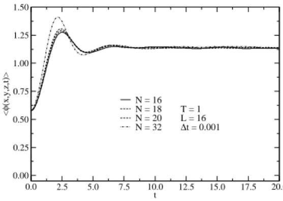
FIG. 3: Solution of the GLL equation with memory and additive noise using the leap frog algorithm for different lattice spacings using counterterms.
0 1 2 3 4 5
m t 0.0
0.2 0.5 0.8 1.0
<
φ
(x,y,z,t)>/m
T/Tc = 0.5
FIG. 4: Solution of Eq. (6) with multiplicative noise using the leap frog algorithm. mis the mass parameter in the original Lagrangian Ref. [3].
the form of Eq. (22). One way to handle this instability, at least for obtaining stable equilibrium solutions, is to intro-duce counterterms inU(φ). The effective three-dimensional theory is super-renormalizable, since only a tadpole diagram
and a setting-sun diagram are divergent and, therefore, to ren-der the theory finite one only needs to subtract fromU(φ)the divergent contributions given by these two diagrams. A more complete discussion on these and explicit expressions for the counterterms can be found in Ref. [6]. In Fig. 3 we present the results of the simulations including the counterterms. One sees that the addition of the regularizing counterterms leads to equilibrium solutions that are independent of lattice spacing.
Finally, we present the result of a simulation using Eq. (6). Our results are shown in Fig. 4 for the broken phase of the model of Ref. [3] with a coupling constant ofλ=0.25. Note that in this case, the dissipation coefficientηis not a free pa-rameter, but was calculated within the model and given by Eq. (7). We have made several tests regarding sensitivity to lattice spacing and time spacings. The general conclusion is that the time step must be considerably smaller than in the case of the equation without noise. For more details and physical interpretation of results, see Ref. [7].
IV. CONCLUSIONS
In this work we have discussed methods for solving numeri-cally GLL equations in three spatial dimensions with memory effects and additive and multiplicative noises. Specifically we have discussed two discretization procedures for the spatial coordinates, finite differences and Fourier collocation. For the discretization of the time variable, we have discussed fi-nite differences and leap frog methods. We have also pointed out the problem of ultraviolet divergences in the solutions of the GLL equations with noise and discussed a method for ob-taining equilibrium solutions that are free from divergences. Explicit solutions were presented for different cases. Most of our attention was on obtaining stable and converging equilib-rium solutions.
V. ACKNOWLEDGEMENT
Work partially supported by CNPq and FAPESP.
[1] A.J. Bray, Adv. Phys.43, 357 (1994).
[2] P. C. Hohenberg, and B. I. Halperin, Rev. Mod. Phys.49, 435 (1977).
[3] M. Gleiser and R.O. Ramos, Phys. Rev. D50, 4 (1994). [4] N.C. Cassol-Seewald, M.I.M. Copetti and G. Krein, submitted to
pulication.
[5] N.C. Cassol-Seewald,A study on dynamic phase transitions and
Ginzburg-Landau-Langevin stochastic equations, Master Disser-tation, IFT, So Paulo, 2006.
[6] E.S. Fraga, G. Krein, and R.O. Ramos,in preparation.