Stochastic Resonance: The role of
Potential Asymmetry and Non Gaussian Noises
Horacio S. Wio y
and Sebastian Bouzat z Comision Nacional de Energa Atomica,
Centro Atomico Bariloche (CNEA) and Instituto Balseiro (CNEA and UNC) 8400{San Carlos de Bariloche, Argentina.
Received 07 December, 1998
Within the two state theory (TST) for stochastic resonance (SR) we analize two dierent aspects: (a) the extension of the TST in order to include potential asymmetry (i.e.: the states show dierent stabilities); (b) the evaluation of transition rates for systems whose stationary distribution is non Gaussian. We apply the results of (a) to study the role of the potential symmetry for SR in bistable systems, observing that the signal-to-noise ratio increases with the symmetry of the potential of the system indicating that it is this feature that governs the optimization of the response. We apply the results of (b) to discuss SR in situations where we can assume that the noise is non Gaussian, and discuss its relation with experimental results in sensory systems.
I Introduction
The phenomenon of stochastic resonance (SR) has at-tracted considerable interest in the last decade due, among other aspects, to its potential technological ap-plications for optimizing the output signal-to-noise ra-tio (SNR) in nonlinear dynamical systems as well as its relation with some biological mechanisms. The phenomenon shows the counterintuitive role played by noise in nonlinear systems as it contributes to enhance the response of a system subject to a weak external sig-nal. There is a wealth of papers, conference proceedings and reviews on this subject [1], Ref. [2] being the most recent one, showing the large number of applications in science and technology, ranging from paleoclimatol-ogy [3], to electronic circuits [4], lasers [5], chemical systems [6], and the connection with some situations of biological interest (noise-induced information ow in sensory neurons in living systems, the inuence in ion-channel gating or in visual perception) [7]. A tendency shown in recent papers, and determined by the possible technological applications, points towards achieving an enhancement of the system response (that is: obtain-ing a larger output SNR) by means of the couplobtain-ing of
several SR units in what conforms anextended medium
[8, 9, 10].
A vast majority of studies on SR have been done analyzing a paradigmatic system: a bistable one-dimensional double-well system. Among the bistable models there is one that singles out: the two-state model
(TST) [3, 11]. Such a model has proven to be extremely useful for the understanding of the SR phenomenon, of-fering also a simple framework to provide analytical re-sults. Most of the studies have been carried out in the symmetric case. However, even in the earliest account of the TST [3] the possibility of asymmetry was in-troduced with the conclusion that the symmetric case would be the optimal one. Other authors have also (partially) analyzed this case (see references in [2]) for instance considering equal curvatures of the potential wells [12]. A more recent and related work [13] lacks a detailed analysis of the role of the symmetry while other points requiere to be claried.
In almost all descriptions, and particularly within the TST, the transition rates between the two wells are estimated as the inverse of themean rst-passage-time. Such a passage time is evaluated using standard Dedicated to the memory of Prof. W. Meckbach
niques [14, 15, 16], and most specically through the Kramers approximation [17]. In all cases the noises are assumed to be Gaussian [14, 15, 16]. However, recent papers analyze a particular class of Langevin (and its associated Fokker-Planck) equations having non Gaus-sian stationary distribution functions [18], opening the possibility of studying the eect of non Gaussian noises on SR. Such a work is based on the generalized ther-mostatistics proposed by Tsallis [19] that has been suc-cesfully applied to a wide variety of physical systems [20].
In this contribution we start with an analysis of the asymmetrical case, extending the TST approach [3, 11], and deriving general expressions for the power spectral density (psd) and for the SNR for a general two-state system. These results are exploited in order to analyze the dependence of the system response on the noise in-tensity and on the degree of asymmetry for a bistable system, showing the central role played by the potential symmetry. We follow with the evaluation of transition rates (or rst passage times) within the Kramers ap-proximation for systems whose stationary distribution is non Gaussian [18]. These results are used to study the eect of such a form of noise on SR, and to compare with experiments and theoretical analysis on the sen-sory system of a craysh [21]. We show that the system response at large values of the noise is better described by the present approach. Such a result strongly sug-gests a non Gaussian character of the noise in these systems.
II Case of Potential Asymmetry
A. GeneralizedTwo StateMo delWe start considering a system described by a dis-crete random dynamical variable x that adopts two
possible values: c 1 and
c
2, with probabilities n
1;2( t) respectively. Such probabilities satisfy the condition n
1( t)+n
2(
t) = 1. The master equation [14, 15, 16] gov-erning the evolution ofn
1(
t) (and similarly forn 2(
t) = 1,n
1( t)) is dn 1 dt =, dn 2 dt = W 2( t)n
2( t),W
1( t)n
1( t)
= W
2( t),[W
2( t) +W
1( t)]n
1 ; (1) where the W
1;2(
t) are the transition rates out of the x=c
1;2states.
If the system is subject (through one of its parame-ters) to a time dependent signal of the formAcos(!
s t), up to rst order on its amplitude (assumed to be small) the transition rates may be expanded as
W 1(
t) = 1
,
1 Acos(!
s t) W
2(
t) = 2+
2
Acos(! s
t); (2)
where the constants 1;2 and
1;2 depend on the de-tailed structure of the system under study. Here we remark that the
i's, that are the (time independent) values of theW
i's without signal, are in general dier-ent from each other as a consequence of the dierdier-ent stability of the two states, and the same happens to the
i's [3]. These considerations are the main dif-ference between our treatment and that of [11] where both 1 = 2 and 1 =
2, were assumed. Using Eq. (2) we can integrate Eq. (1) with the initial con-ditionx(t
0) = x
0and obtain the conditional probabil-ityn
1( tj x
0 ;t
0). This result will allow us to calculate the autocorrelation function, the power spectral density (psd) and nally the SNR.
We follow the procedure of Ref. [11] to compute the SNR, generalizing it in order to include the asymmet-ric case when
1 6 = 2 and 1 6 =
2. Once Eq. (1) is integrated we can calculate the correlation function hx(t+)x(t)jx
0 ;t
0 ias c
hx(t+)x(t)jx 0
;t 0
i = c
2 1 n
1( t+ jc
1 ;t)n
1( tjx
0 ;t 0) +c 1 c 2 n 1( t+ jc
2 ;t)n
2( tjx
0 ;t
0) + c 1 c 2 n 2( t+ jc
1 ;t)n
1( tjx
0 ;t 0) +c 2 2 n 2(
t+ jc 2
;t)n 2(
tjx 0
;t
For the t-averaged correlation function C() = hlimt
0!,1
hx(t+)x(t)jx 0
;t 0
iit, we obtain C() =R
0 +
R 1exp(
,jj) +R 2cos(
!s): (4) Here=
1+
2 and the constants
Ri are given by R 0 = c 2 1+ c 1 2 1+ 2 2 R
1 = (
c 2 ,c 1) 2 1 2 2 +
O(A 2) R 2 = A 2( c 1 ,c 2) 2( 2 1+ 1 2) 2 2 2( 2+ ! 2) : (5)
Then, noting that R
0 is just the square of the mean value ofxin the absence of signal (R
0= hxi
2 jA
=0), we compute the t-averaged psd
hS~(!)it
as the Fourier transform of (C(),R
0). After that, we compute the one-sidedt-averaged psd (S(!)), dened for!>0, as
S(!) =hS~(!)it+hS~(,!)it: (6) We nally get
S(!) = 4R 1
(
2+ !
2) + 2 R
2
(!,!s): (7) In the one-sided t-averaged psd (Eq. (7)), two contri-butions can be distinguished: the signal output which is given by the function centered at the signal fre-quency and the broadband noise output, given by a dominant (O(A
0)) Lorentzian term pluss some less im-portant (O(A
2)) terms that have been neglected. If when calculating the power spectrum, instead of (C(),R
0), only
C() is considered, an extra term (4 R
0
(!)) appears in Eq. (7). Note that a non van-ishing value ofR
0can be caused either by an asymmet-ric choice of the values of c
1 and c 2 ( c 1 6 =,c
2) or by a dierence in the stabilities of both states (
1
6
= 2) even when c
1 = ,c
2 is considered. If we consider the symmetric case (
1=
2 ~
0
=2 and 1= 2 ~ 1 =2) and also xc
2= ,c
1
c, we recover exactly the result of [11].
For the general asymmetric case we dene R, the SNR, as the ratio of the strength of the output signal and the broadband noise output evaluated at the signal frequency, obtaining R= R 2 R 1 2 ( 2 +! 2 s ) = A 2 ( 2 1+ 1 2) 2 4 1 2( 1+ 2) : (8)
This result shows that the well known independence of the SNR on the signal frequency for small signal am-plitude for symmetric systems [11] is also found to be valid when the symmetry is broken. It is worth remark-ing that when we consider the symmetrical case all our results reduce to those in [11].
In the case analyzed in the following subsection we will work with R=A
2 instead of
R and rename it: R=A
2
!R, that now will characterize the SNR inde-pendently of both the signal frequency and amplitude. Such a case corresponds to the application of this the-ory to study the SR of a double-well system in order to analyze the role played by the asymmetry in a simple standard example.
B. Application to a Simple Bistable System
Here we apply the theory described in the previous subsection to the following stochastic system
_
u(t) =,(u 2
,1)(u+a) +S(t) + p
2(t); (9) where (t) is a Gaussian white noise of zero mean and correlation h(t)(t
0)
i= (t,t
0). The corresponding quartic potential is
V(u) = u 4 4 + au 3 3 , u 2
2 ,(a+S(t))u (10) ForS(t) = 0 it has minima atu=1 and a maximum atu=,a and it is symmetric aroundu= 0 fora= 0. For S(t) 6= 0 but small, up to rst order in S(t), the extrema are located at
u 1= 1 +
S(t) 2(1 +a)
; u 2=
,1 + S(t) 2(1,a) and um=,a,
S(t) 1,a
2 (11)
In Fig. 1, we depict the form of the potential for the symmetric situation (a= 0 with S(t) = 0) and for an asymmetric case for two dierent values of the signal.
In order to apply the theory of the previous sec-tion we set S(t) =Acos(!st) and assume that (!s)
c
Wu 1
!u 2
W
1= p
jV 00(
um)jV 00(
u 1) 2
exp
,
(V(um),V(u 1))
Wu 2!u
1
W
2= p
jV 00(
um)jV 00(
u 2) 2
exp ,
(V(um),V(u 2))
; (12)
d where V
00 is the second derivative of
V with respect to u. The parametersi and i result to be functions of aandthat can be analytically calculated as
1 =
W 1
jS
(t)=0 ;
1= ,
dW 1 dS(t)
jS (t)=0
2 = W
2 jS
(t)=0 ;
2= dW
2 dS(t)
jS (t)=0
: (13) Then we can compute the SNR (as explained in the previous section) as a function of a and the noise in-tensity. The parameteracharacterizes the symmetry of the potential as follows: setting a = 0 corresponds to modulating around a symmetric situation in which both states are equally stable, and a>0 corresponds to modulating around a situation in which the state c
1 (the well around u
1) is more stable than the state c
2. Finally, a < 0 corresponds to modulating around the opposite situation where the state c
2 is the more sta-ble one. However, as the system is invariant under the simultaneous transformations a ! ,a;u ! ,u, and S(t) !,S(t), the results of R for a are the same to those for ,a and hence, we will only consider the case a>0.
Figure 1. Potential V(x) for dierent values of the
param-eters.
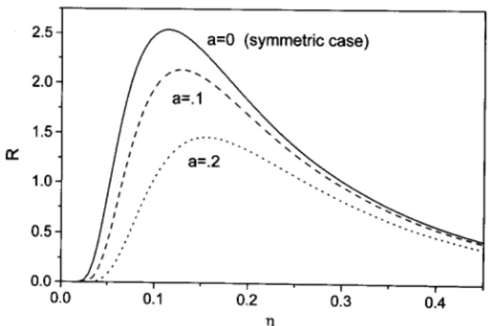
In Fig. 2 we show the results ofR() for dierent values ofa. Note that each curve shows an optimum noise intensity where the SNR has a maximum; this is the typical characteristic of the SR phenomenon. Fur-thermore, it can be appreciated that the value of the maximum ofRincreases with the symmetry of the sys-tem (i. e. with the proximity ofato zero). Actually, for any given value of,Ris maximized by settinga= 0. Hence the symmetric situation is the more favorable one for the SR phenomenon.
Figure 2. SNR as a function of the noise intensity for dif-ferent values of the parametera.
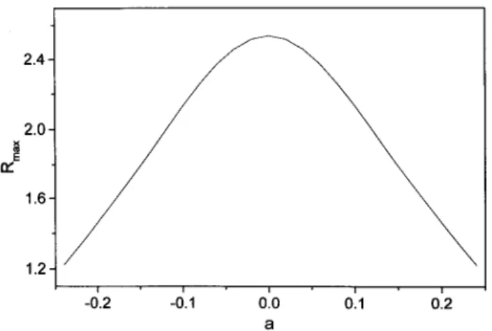
In Fig. 3 we show the value of the maximum ofR plotted as a function ofa. The exact analytical expres-sion ofRas a function ofaandis complicated and we will not give it here. The optimization ofRthat occurs in the symmetric case (a= 0) is apparent.
Figure 3. Maximum of R (Rmax) as a function of a. The
maximun of Rmax occures for a= 0 which corresponds to
the modulation around the symmetric situation.
III First-Passage Time and SR
with non Gaussian Noises
Traditionally, a tight connection between standard lin-ear Fokker-Planck or Langevin equations and Gaus-sian (Boltzmann-Gibbs like) distributions was assumed. However, some recent papers have shown that there is an entire family of microscopic Langevin equations (with its associated Fokker-Planck equations) such that the resulting process has a Tsallis distribution [19] on the macroscopic level [18, 23, 24]. One of the possible interpretations is that the noise source is non Gaussian. Here we present a brief account of the calculation of the transition rates (or rst passage times) within the Kramers approximation for systems whose station-ary distribution is non Gaussian, and the use of thoseresults to analyze the SR and the eect on the SNR. A detailed account of this analysis will be presented elsewhere [25].
In Ref. [18] it was shown that a Fokker-Planck equa-tion with constant diusion coecient D (that mea-sures the intensity of uctuations)
@ @t
P(x;t) = @ @x
@V(x)
@x
P(x;t)
+D @
2 @x 2
P(x;t); (14) with the "generalized potential"
V(x) = 1
(q,1) ln[1 +
(q,1)U(x)]; (15) has the following stationary distribution [18] ( = 1=D, withD the noise intensity)
Pst(x) = N exp(,V(x)) = N [1 +(q,1)U(x)]
1 1,q
; (16) where N is a normalization factor. The results of Ref. [18] have two alternative interpretations. The obvious one corresponds to the study of diusion in a potential given byV(x), induced by a white Gaussian noise. The other possibility is to consider that we are studying dif-fusion in a potential given by U(x) and subject to a non-Gaussian noise.
It is well known that for a potential like the one in Fig. 1, with a stationary distribution Pst(x) exp[,V(z)=D], the rst{passage time is given by [14, 15, 16, 17] (here we consider the symmetric case, hence a=,um = 0)
c
T(u 2
!x 0) = 1
D Z x
0
u2
dyexp[V(y)=D] Z y
,1
dzexp[,V(z)=D]: (17)
When we replace the form of the potential given in Eq. (15), and make the integrals using the standard stepeest descent method, the rst passage time adopts the form
T(u 2
!0) = N D
1 +(q,1)U(u 2) 1 +(q,1)U(0)
1 1,q
4(1 +(q,1)U(u 2))(1 +
(q,1)U(0))
2 U"(u
2) jU"(0)j
1=2
; (18)
with
N = Z
1 ,1
dy[1 + (q,1)y 2]
1 1,q
Z p
1 1,q ,
p 1 1,q
dz[1,(q,1)z 2]
1 q ,1
: (19)
In the limitq!1 it is easy to see thatN !, and also thatT(u 2
With the previous results we are in position to evaluate the transition rates and to write the expresions for the psd S(!) (Eq.(7)) and the SNR (Eq. (8)). The expression forRresults (in our caseU(0) = 0)
R
A 2 16ND
2( q+ 1)
2 p
U"(u 2)
jU"(0)j
1 + q,1 D
U(u 2)
,
1 1,q
, 1 2
: (20)
d In the limitq !1 it reduces to the well known result [11].
However, it is still necessary to correct one draw-back: the above indicated results are dependent on the energy reference level. As was disscused in [26], in order to avoid some consequences for the use of a nonextensive form of the entropy (the distributions are not invariant under uniform translations of the energy spectrum; the non-preservation of the norm; and that the rst principle of thermodynamics does not preserve macroscopically the same form it has microscopically), it is requiered what the authors called the thirdchoice for the internal energy constraint. The complication is that many quantities can only be obtained in a self{ consisting form. As within the second choice all cal-culations are much easier, it is better to work within it and afterwards to establish the relation between the parameters. When we consider such an approach, it becomes necessary to relate the value of the parameter from the third choice () with that from the second one (~).
According to [26] we have the relation between the actual (third choice) value of and the "operational" (second choice) value ~ given by
=
~
h P
p (2) j (~
) q
i 2 P
p (2) j (~
) q
,(1,q)~U (2)(~
)
; (21)
wherep (2) j (~
) andU (2)(~
) are the probabilities and av-eraged potential evaluated within the "second choice". Clearly, forq!1 we have !~= 1=D.
Taking into account the indicated correction, we can calculate the SNR according to Eq. (20), and correct the values of according to Eq. (21). It is worth to point out that not all the values ofqare allowed, with some limits imposed by the conditions that the prob-abilities be positive denite and that the SNR do not diverge for D!0. Such conditions yield 1q5=3.
At this point it becomes necessary to connect the
present bistable model with the excitable one studied in Ref. [21]. In the indicated reference, the SNR is ob-tained via a Fourier expansion of the time periodic rate (t), and a Kramers-type (time dependent) formula to evaluate the rst few coecients. The result is an ex-pression for the SNR similar to the one arising from a TST approach [11]. The only dierence is a factor 2 in the denominator of the exponent (see Eq. (10) in [21]). Hence, it is clear that we can use our results above as an approximation of the Kramers time and as a (simple) modelization of the SNR in the indicated situation
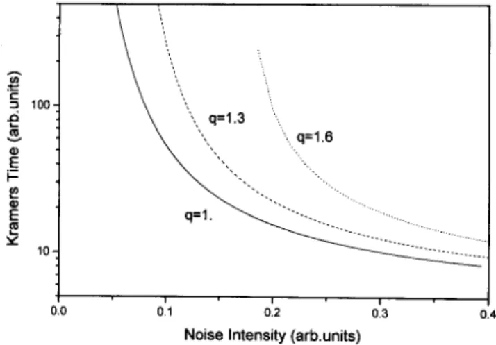
Figure 4. Kramers time (Eq. (18)) as a function of the noise intensityDfor dierent values ofq.
there. Such a result strongly suggests a non Gaussian character of the noise in these kind of systems.
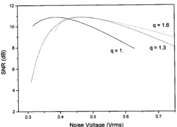
Figure 5. SNR as a function of the rms noise voltage (de-ned asp
h 2
i= p
2D) for dierent values ofq.
IV Conclusions
In this contribution we have analyzed the role of poten-tial symmetry in the SR for bistable systems without spatial extention, for the case of small signal ampli-tudes. We have extended the TST of SR [3, 11] in or-der to include situations with potential asymmetry. We have shown that the results for SNR for general asym-metric systems are independent of the signal frequency. An important aspect of our treatment is that we have found a way to eectively reduce any bistable system to a discrete two{state one, however for the case of small signal amplitudes. We have used this extended theory to analyze the SR of a simple system: a double-well potential, and have found that the symmetric situation is the optimal one in order to improve the SNR. It is worth mentioning that we have obtained essentialy the same results in other dierent bistable systems, partic-ualrly in spatially extended systems. Furthermore this behavior seems to be independent of the way in which the signal is introduced in the system [22].
Here we want to remark that these results diers from those found in [13]. In one hand our result for the SNR shows that the well known independence of the SNR on the signal frequency for a small signal ampli-tude for symmetric systems [11] is also found to be valid when the symmetry is broken. On the other hand, in
[10, 22] it was shown that the FitzHugh-Nagumo model, in the bistable regime, has a (nonequilibrium) potential (although the system is nongradient), indicating that the claim in [13] of studying a \nonpotential system" is wrong.
The second aspect we have analyzed, is related with the possible non Gaussian character of the noise source. In general, the transition rates between the two wells are estimated as the inverse of the Kramers decay time [17], evaluated with the assumption that the noise is Gaussiann [14, 15, 16]. We have used recent results, where a particular class of Langevin equations hav-ing non Gaussian stationary distribution functions were studied [18]. The evaluation of the decay time within a Kramers approximation allows us to obtain all the rele-vant quantities to disscus SR within such a framework: the correlation functions, the psd, and the SNR. All those results reduce to the known ones as the "Tsallis parameter" [19, 20] q ! 1. The results for the SNR as a function of the noise intensity D clearly indicates a marked inuence of the value of q. The present re-sult oers a better description of the SNR for large values of D than the usual one when compared with experimetal results [21], indicating a possible non Gaus-sian behaviour of the noises. The lack of agreement for low noise intensity can be caused (as argued in [21]) to extra noise contributions due to the spontaneous ring of the neuron.
Finally, we want to remark that the study of both aspects, in addition to the analysis of their inuence in SR, have a larger relevance than pure theoretical spec-ulations. For instance, bistable asymmetric situations provide the appropriate framework for describing SR in voltage{dependent ion channels, as proposed in [7]. In those systems, the conducting state is associated to a higher-energy well than the non{conducting one. Also the experiments on sensory systems like those in [21] and related ones, show the need to go beyond the stan-dard approaches in order to obtain better descriptions of the experimental data.
Grunfeld for a revision of the manuscript. Support from CONICET, through grant PIP Nro.4593/96, ANPCyT, through grant PICT 97 Nr.03-00000-00988, and CEB, Bariloche, are also acknowledged.
References
[1] Proc. NATO Adv. Res. Work. on Stochastic Resonance in Physics and Biology, F. Moss, et al., eds., J. Stat. Phys. 70 No. 1/2 (1993); Proc. 2nd. Int. Work. on Fluctuations in Physics and Biology, A. Bulsara et al, eds., Nuovo Cim. D17(1995).
[2] L. Gammaitoni, P. Hanggi, P. Jung and F. Marchesoni, Rev. Mod. Phys.70223 (1988).
[3] C. Nicolis, Tellus34, 1 (1982).
[4] S. Fauve and F. Heslot, Phys. Lett. A 97, 5 (1983);
R.N. Mantegna and B. Spagnolo, Phys. Rev. E 49,
R1792 (1994); V.S. Anishchenko,M.A. Safonova and L.O. Chua, Int. J. Bifurcation and Chaos Appli. Sci. Eng.4, 441 (1994).
[5] J.M. Iannelli, A. Yariv, T.R. Chen and Y.H. Zhuang, Appl. Phys. Lett. 65, 1983 (1994); A. Simon and A.
Libchaber, Phys. Rev. Lett.69, 3375 (1992).
[6] A. Guderian, G. Dechert, K. Zeyer and F. Schneider; J. Phys. Chem.100, 4437 (1996); A. Forster, M. Merget
and F. Schneider; J. Phys. Chem. 100, 4442 (1996);
W. Hohmann, J. Muller and F. W. Schneider; J. Phys. Chem. 100, 5388 (1996); V. Petrov, Q.Ouyang and
H.L. Swinney, Nature388, 655 (1997); and P. De
Kep-per and S. Muller, private communication.
[7] J. K. Douglas, L. Wilkens, E. Pantazelou & F. Moss, Nature365, 337-340 (1993); H.A. Braun, H. Wissing,
K. Schafer & M.C. Hirsch, Nature367, 270-273 (1994);
I.L. Kruglikov & H. Dertinger, Bioelectromag.15,
539-547 (1994); F. Moss & X. Pei, Nature 376, 211-212
(1995); J. J. Collins, C.C. Chow & T.T. Imho, Nature
376, 236-238 (1995); S. M. Bezrukov & I. Vodyanoy,
Nature378, 362-364 (1995); J. J. Collins, T.T. Imho
& P. Grigg, Nature 383, 770-770 (1996); B.J.
Gluck-man, T.J. Neto, E.J. Neel, W.L. Ditto, M.L. Spano & S.J. Schi, Phys. Rev. Lett. 77, 4098-4101 (1996);
S. M. Bezrukov & I. Vodyanoy, Nature 385, 319-321
(1997); R.D. Astumian, R.K. Adair & J.C. Weaver, Nature 388, 632-633 (1997). E. Simonotto, M. Riani,
C. Seife, M. Roberts, J. Twitty & F. Moss, Phys. Rev. Lett. 78, 1186-1189 (1997); P.C. Gailey, A. Neiman,
J.J. Collins & F. Moss, Phys. Rev. Lett.79, 4701-4704
(1997).
[8] A. Bulsara and G. Schmera, Phys. Rev. E 47, 3734
(1993); P. Jung, U. Behn, E. Pantazelou and F. Moss, Phys. Rev. A46, R1709 (1992); Jung and Mayer-Kress,
Phys. Rev. Lett. 74, 208 (1995); J.F. Lindner, B.K.
Meadows, W.L. Ditto, M.E. Inchiosa and A. Bulsara, Phys. Rev. Lett.75, 3 (1995), and Phys. Rev. E 53,
2081 (1996); F. Marchesoni, L. Gammaitoni and A.R. Bulsara; Phys. Rev. Lett.76, 2609 (1996); J. Vilar and
J. Rubi; Phys. Rev. Lett.78, 886 (1997).
[9] H. S. Wio, Phys. Rev. E 54, R3045 (1996); H.
S. Wio and F. Castelpoggi, Proc. Conf. UPoN'96, C.R.Doering, L.B.Kiss and M.Schlesinger Eds. (World Scientic, Singapore, 1997), pg. 229; F. Castelpoggi and H.S. Wio, Europhysics Letters 38, 91 (1997); F.
Castelpoggi and H. S. Wio, Phys. Rev. E 57, 5112
(1998); M. Kuperman, H.S. Wio, G. Izus and R. Deza, Phys. Rev. E57, 5122 (1998); M. Kuperman, H.S. Wio,
G. Izus, R. Deza and F. Castelpoggi, Physica A257,
275 (1998).
[10] S. Bouzat and H. S. Wio, submitted to Physica A (1998); S. Bouzat and H. S. Wio, Phys. Lett. A (1998) in press.
[11] B. McNamara and K. Wiesenfeld, Phys. Rev. A 39,
4854 (1989).
[12] P. Jung and R. Bartussek, inFluctuations and Order: The New Synthesis, edited by M. Millones (Springer, New York, Berlin), pg. 35.
[13] T. Alarcon, A. Perez-Madrid and J.M. Rub, Phys. Rev. E57, 4979 (1998).
[14] C. W. Gardiner; Handbook of Stochastic Methods, 2nd Ed. (Springer-Verlag, Berlin, 1985).
[15] N. van Kampen; Stochastic Processes in Physics and Chemistry, (North Holland, 1982).
[16] H. S. Wio, An Introduction to Stochastic Processes and Nonequilibrium Statistical Physics (World Scien-tic, Singapore, 1994).
[17] P. Hanggi, P. Talkner and M. Borkovec, Rev. Mod. Phys,62, 251 (1990).
[18] L. Borland, Phys. Lett. A245, 67 (1998); L. Borland
Phys. Rev. E57, 6634 (1998).
[19] C. Tsallis, J. Stat. Phys52, 479 (1988); E. M. F.
Cu-rado and C. Tsallis, J. Phys. A24, L69 (1991); ibidem 24, 3187 (1991), ibidem 25, 1019 (1992).
[20] A.R. Plastino and A. Plastino, Phys. Lett. A 174,
384 (1993); A.R. Plastino and A. Plastino, Physica A 222, 347 (1995); D.H. Zanette and P.A. Alemany,
Phys. Rev. Lett.75, 366 (1995); B.M. Boghosian, Phys.
Rev. E53, 4754 (1996); C. Tsallis and D.J. Bukman,
Phys. Rev. E54, R2197 (1996); V.H. Hamity and D.E.
Barraco, Phys. Rev. Lett.76, 4664 (1996); A.K.
Ra-jagopal, Phys. Rev. Lett.76, 3469 (1996); C. Tsallis
and A.M.C. de Souza, Phys. Lett. A235, 444 (1997).
[21] K. Wiesenfeld, D. Pierson, E. Pantazelou, Ch. Dames and F. Moss, Phys. Rev. Lett.72, 2125 (1994).
[22] S. Bouzat and H. S. Wio, Stochastic resonance in ex-tended bistable systems: the role of potential symmetry, submitted (1998).
[23] D.A. Stariolo, Phys. Lett. A185, 262 (1994).
[24] G. Kaniadakis and P. Quarati, Physica A 237, 229
(1997).
[25] H. S. Wio and C. Tsallis,Decay Times and Stochastic Resonance Within A Non extensive Thermostatistical Framework, in preparation.
[26] C. Tsallis, R.S. Mendes and A.R. Plastino, Physica A