Ozone variability in the troposphere and the stratosphere from the first six years of IASI observations (2008–2013)

(1)

ACPD

15, 27575–27625, 2015

Ozone variability in the troposphere and the stratosphere from

the first six years of IASI observations

C. Wespes et al.

Title Page

Abstract Introduction

Conclusions References

Tables Figures

◭ ◮

Back Close

Full Screen / Esc

Printer-friendly Version

Interactive Discussion

Discussion

P

a

per

|

Discussion

P

a

per

|

Discussion

P

a

per

|

Discussion

P

a

per

|

Atmos. Chem. Phys. Discuss., 15, 27575–27625, 2015 www.atmos-chem-phys-discuss.net/15/27575/2015/ doi:10.5194/acpd-15-27575-2015

This discussion paper is/has been under review for the journal Atmospheric Chemistry and Physics (ACP). Please refer to the corresponding final paper in ACP if available.

Ozone variability in the troposphere and

the stratosphere from the first six years of

IASI observations (2008–2013)

C. Wespes1, P.-F. Coheur1, L. K. Emmons2, D. Hurtmans1, S. Safieddine3,

C. Clerbaux1,3, and D. P. Edwards2

1

Spectroscopie de l’Atmosphère, Service de Chimie Quantique et Photophysique, Université Libre de Bruxelles (U.L.B.), Brussels, Belgium

2

National Center for Atmospheric Research, Boulder, CO, USA

3

Sorbonne Universités, UPMC Univ. Paris 06; Université Versailles St-Quentin; CNRS/INSU, LATMOS-IPSL, Paris, France

Received: 14 August 2015 – Accepted: 19 September 2015 – Published: 14 October 2015

Correspondence to: C. Wespes ([email protected]) and P.-F. Coheur ([email protected])

(2)

ACPD

15, 27575–27625, 2015

C. Wespes et al.

Title Page

Tables Figures

◭ ◮

Back Close

Full Screen / Esc

Discussion

P

a

per

|

Discussion

P

a

per

|

Discussion

P

a

per

|

Discussion

P

a

per

|

Abstract

In this paper, we assess how daily ozone (O₃) measurements from the Infrared At-mospheric Sounding Interferometer (IASI) on MetOp-A platform can contribute to the analyses of the processes driving O₃variability in the troposphere and the stratosphere and, in the future, to the monitoring of long-term trends. The time development of O₃

5

during the first 6 years of IASI (2008–2013) operation is investigated with multivari-ate regressions separmultivari-ately in four different layers (ground–300, 300–150, 150–25, 25– 3 hPa), by adjusting to the daily time series averaged in 20◦_{zonal bands, seasonal and}

linear trend terms along with important geophysical drivers of O₃ variation (e.g. solar flux, quasi biennial oscillations). The regression model is shown to perform generally

10

very well with a strong dominance of the annual harmonic terms and significant con-tributions from O₃ drivers, in particular in the equatorial region where the QBO and the solar flux contribution dominate. More particularly, despite the short period of IASI dataset available to now, two noticeable statistically significant apparent trends are in-ferred from the daily IASI measurements: a positive trend in the upper stratosphere

15

(e.g. 1.74±0.77 DU yr−1 between 30–50◦S) which is consistent with the turnaround

for stratospheric O₃ recovery, and a negative trend in the troposphere at the mid-and high northern latitudes (e.g.−0.26±0.11 DU yr−1between 30–50◦N), especially during

summer and probably linked to the impact of decreasing ozone precursor emissions. The impact of the high temporal sampling of IASI on the uncertainty in the

determina-20

tion of O₃ trend has been further explored by performing multivariate regressions on IASI monthly averages and on ground-based FTIR measurements.

1 Introduction

Global climate change is one of the most important environmental problems of today and monitoring the behavior of the atmospheric constituents (radiatively active gases

25

(3)

cli-ACPD

15, 27575–27625, 2015

C. Wespes et al.

Title Page

Tables Figures

◭ ◮

Back Close

Full Screen / Esc

Discussion

P

a

per

|

Discussion

P

a

per

|

Discussion

P

a

per

|

Discussion

P

a

per

|

mate and apprehend future climate changes. Long-term measurements of these gases are necessary to study the evolution of their abundance, changing sources and sinks in the atmosphere.

As a reactive trace gas present simultaneously in the troposphere and in the strato-sphere, O₃plays a significant role in atmospheric radiative forcing, atmospheric

chem-5

istry and air quality. In the stratosphere, O₃is sensitive to changes in (photo-)chemical and dynamical processes and, as a result, present large variations on seasonal and annual time scales. Measurements of O₃total column have indicated a downward trend in stratospheric ozone over the period from 1980s to the late 1990s relative to the pre-1980 values, which is due to the growth of the reactive bromine and chlorine species

10

following anthropogenic emissions during that period (WMO, 2003). In response to the 1987 Montreal Protocol and its amendments, with a reduction of the Ozone-Depleting Substances (ODS; Newchurch et al., 2003), a recovery of stratospheric ozone con-centrations to the pre-1980 values is expected (Hofmann, 1996). While earlier works have debated a probable turnaround for the ozone hole recovery (e.g. Hadjinicolaou

15

et al., 2005; Reinsel et al., 2002; Stolarski and Frith, 2006), WMO already indicated in 2007 that the total ozone in the 2002–2005 period was no longer decreasing, reflect-ing such a turnaround. Since then several studies have shown successful identification of ozone recovery over Antarctica and over northern latitudes (e.g. Mäder et al., 2010; Salby et al., 2011; WMO, 2011; Kuttippurath et al., 2013; Knibbe et al., 2014; Shepherd

20

et al., 2014). Nevertheless, the most recent papers as well as the WMO 2014 ozone assessment have warned for various reasons against overly optimistic conclusions with regard to a possible increase in Antarctic stratospheric ozone (Kramarova et al., 2014 ; WMO, 2014; Knibbe et al., 2014; de Laat et al., 2015; Kuttippurath et al., 2015; Varai et al., 2015). The causes of the observed stratospheric O₃changes are hard to isolate

25

(4)

ACPD

15, 27575–27625, 2015

C. Wespes et al.

Title Page

Tables Figures

◭ ◮

Back Close

Full Screen / Esc

Discussion

P

a

per

|

Discussion

P

a

per

|

Discussion

P

a

per

|

Discussion

P

a

per

|

of precursors, long-range transport, stratosphere–troposphere – STE – exchanges), which are all strongly variable temporally and spatially (e.g. Logan et al., 2012; Hess and Zbinden, 2013; Neu et al., 2014). Overall, there are still today large differences in the value of the O₃trends determined from independent studies and datasets in both the stratosphere and the troposphere (e.g. Oltmans et al., 1998, 2006; Randel and

5

Wu, 2007; Gardiner et al., 2008; Vigouroux et al., 2008; Jiang et al., 2008; Kyrölä et al., 2010; Vigouroux et al., 2014). In order to improve on this and because O₃ has been recognized as an GCOS Essential Climate Variables (ECVs), the scientific community has underlined the need of acquiring high quality global, long-term and homogenized ozone profile records from satellites (Randel and Wu, 2007; Jones et al., 2009; WMO,

10

2007, 2011, 2014). This specifically has resulted in the ESA Ozone Climate Change Initiative (O₃-CCI; http://www.esa-ozone-cci.org/).

The Infrared Atmospheric Sounding Interferometer (IASI) onboard the polar orbiting MetOp, with its unprecedented spatiotemporal sampling of the globe, its high radio-metric stability and the long duration of its program (3 successive instruments to cover

15

15 years) provides in principle an excellent means to contribute to the analyses of the O₃variability and trends. This is further strengthened by the possibility to discriminate well with IASI, the O₃ distributions and variability in the troposphere and the strato-sphere, as shown in earlier studies (Boynard et al., 2009; Wespes et al., 2009, 2012; Dufour et al., 2010 ; Barret et al., 2011; Scannell et al., 2012; Safieddine et al., 2013).

20

Here, we use the first 6 years (2008–2013) of the new O₃ dataset provided by IASI on MetOp-A to perform a first analysis of the O₃time development in the stratosphere and in the troposphere. This is achieved globally by using zonal averages in 20◦_latitude

bands and a multivariate linear regression model which accounts for various natural cy-cles affecting O₃. We also explore in this paper to which extent the exceptional temporal

25

sampling of IASI can counterbalance the short period of data available for assessing trends in partial columns.

(5)

ACPD

15, 27575–27625, 2015

C. Wespes et al.

Title Page

Tables Figures

◭ ◮

Back Close

Full Screen / Esc

Discussion

P

a

per

|

Discussion

P

a

per

|

Discussion

P

a

per

|

Discussion

P

a

per

|

In Sect. 4, we evaluate how the ozone natural variability is captured by IASI and we present the time evolution of the retrieved O₃profiles and of four partial columns (Up-per Stratosphere –US–; Middle-Low Stratosphere –MLS–; Up(Up-per Troposphere Lower Stratosphere –UTLS–; Middle-Low Troposphere –MLT–) using 20◦latitudinal averages on a daily basis. The apparent dynamical and chemical processes in each latitude band

5

and vertical layer are then analyzed on the basis of the multiple regression results us-ing a series of common geophysical variables. The “standard” contributors in the fitted time series, as well as a linear trend term, are analyzed in the specified altitude lay-ers. Finally, the trends inferred from IASI are compared against those from FTIR for six stations in the Northern Hemisphere.

10

2 IASI measurements and retrieval method

IASI measures the thermal infrared emission of the Earth–atmosphere between 645 and 2760 cm−1with a field of view of 2×2 circular pixels on the ground, each of 12 km

diameter at nadir. The IASI measurements are taken every 50 km along the track of the satellite at nadir, but also across-track over a swath width of 2200 km. IASI provides

15

a global coverage twice a day with overpass times at 09:30 and 21:30 mean local solar time. The instrument is also characterized by a high spectral resolution which allows the retrieval of numerous gas-phase species (e.g. Clerbaux et al., 2009; Clarisse et al., 2012).

Ozone profiles are retrieved with the Fast Optimal Retrievals on Layers for IASI

20

(FORLI) software developed at ULB/LATMOS. FORLI relies on a fast radiative transfer and on a retrieval methodology based on the Optimal Estimation Method (Rodgers, 2000). In the version used in this study (FORLI-O₃ v20 100 815), the O₃ profile is re-trieved for individual IASI measurement on a uniform 1 km vertical grid on 40 layers from surface up to 40 km. The retrieval parameters and performances are detailed in

25

(6)

satel-ACPD

15, 27575–27625, 2015

C. Wespes et al.

Title Page

Tables Figures

◭ ◮

Back Close

Full Screen / Esc

Discussion

P

a

per

|

Discussion

P

a

per

|

Discussion

P

a

per

|

Discussion

P

a

per

|

lite observations (Anton et al., 2011; Dufour et al., 2012; Gazeaux et al., 2012; Par-rington et al., 2012; Pommier et al., 2012; Scannell et al., 2012; Oetjen et al., 2014). Generally, the results show good agreements between FORLI-O₃ and independent measurements with a low bias (<10 %) in the total column and in the vertical pro-file, except in UTLS where a positive bias of 10–15 % is reported (Dufour et al., 2012;

5

Gazeaux et al., 2012; Oetjen et al., 2014).

In this study, only daytime O₃IASI observations from good spectral fits (RMS of the spectral residual lower than 3.5_×10−8_W_/_(cm2_{sr cm}−1_{)) have been analyzed. Daytime}

IASI observations are characterized by a better vertical sensitivity to the troposphere associated with a higher surface temperature and a higher thermal contrast (Clerbaux

10

et al., 2009; Boynard et al., 2009). Furthermore, cloud contaminated scenes with cloud cover<13 % (Hurtmans et al., 2012) were removed using cloud information from the Eumetcast operational processing (August et al., 2012).

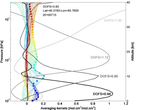
An example of typical FORLI-O₃ averaging kernel functions for one mid-latitude ob-servation in July (45◦N/66◦E) is represented on Fig. 1. The layers have been defined

15

as: ground–300 hPa (MLT), 300–150 hPa (UTLS), 150–25 hPa (MLS) and above 25 hPa (US), so that they are characterized by a DOFS (Degrees Of Freedom for Signal) close to 1 with a maximum sensitivity approximatively in the middle of the layers, except for the 300–150 hPa layer which has a reduced sensitivity. Taken globally, the DOFS for the entire profile ranges from _∼2.5 in cold polar regions to _∼4.5 in hot tropical

re-20

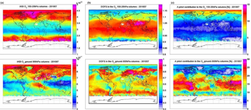
gions, depending mostly on surface temperature, with a maximum sensitivity in the upper troposphere and in the lower stratosphere (Hurtmans et al., 2012). In the MLT, a maximum of sensitivity peaks around 6–8 km altitude for almost all situations (We-spes et al., 2012). Figure 2 presents July 2010 global maps of averaged FORLI-O₃ partial columns for two partial layers (MLT and MLS), and of the associated DOFS and

25

(7)

ACPD

15, 27575–27625, 2015

C. Wespes et al.

Title Page

Tables Figures

◭ ◮

Back Close

Full Screen / Esc

Discussion

P

a

per

|

Discussion

P

a

per

|

Discussion

P

a

per

|

Discussion

P

a

per

|

medium humidity, such as the mid-latitude continental Northern Hemisphere (N.H.) (Clerbaux et al., 2009). Lower DOFS values in the intertropical belt are explained by an overlapping from water vapor lines. In contrast, the DOFS for the MLS are glob-ally almost constant and close to one, with only slightly lower values (0.9) over polar regions. The a priori contribution is anti-correlated with the sensitivity, as expected. It

5

ranges between a few % to∼30 % and does not exceed 20 % on 20◦ zonal averages

in the troposphere (see Supplement; Fig. S3, dashed lines), while the a priori contri-bution is smaller than_∼12 % in the middle stratosphere. These findings indicate that the IASI MLS time series should accurately represent stratospheric variations, while the time series in the troposphere may reflect to some extent variations from the

up-10

per layers in addition to the real variability in the troposphere. In order to quantify this effect, the contribution of the stratosphere in the tropospheric ozone as seen by IASI has been estimated with a global 3-D chemical transport model (MOZART-4). We show that it varies between 30 and 60 % depending on latitude and season. Details of the model-observation comparisons can be found in the Supplement (see Figs. S2 and

15

S3). The fact that IASI MLT O₃is “contaminated” to a significant extend with variations in stratospheric O₃should be kept in mind when analyzing IASI MLT O₃.

3 Fitting method

3.1 Statistical model

In order to characterize the changes in ozone measured by IASI and to allow

separa-20

(8)

ACPD

15, 27575–27625, 2015

C. Wespes et al.

Title Page

Tables Figures

◭ ◮

Back Close

Full Screen / Esc

Discussion

P

a

per

|

Discussion

P

a

per

|

Discussion

P

a

per

|

Discussion

P

a

per

|

fitting of daily (or monthly) median partial columns in different latitude band following:

O

3(t)=Cst+x1·trend+

X

n=1,2[an·cos(nωt)+bn·sin(nωt)]+

m

X

j=2

xjXnorm,j(t)+ε(t) (1)

wheretis the number of days (or months),x₁is the 6 year trend coefficient in the data,

ω=2π/365.25 for the daily model (or 2π/12 for the monthly model) and X_norm,_j are independent geophysical variables, the so-called “explanatory variables” or “proxies”,

5

which are in this study normalized over the period of IASI observation (2008–2013), as:

X_norm(t)=2 (X(t)₋X_median)/(X_max−Xmin) (2)

ε(t) in Eq. (1) represents the residual variation which is not described by the model and which is assumed to be autoregressive with time lag of 1 day (or 1 month). The constant

10

term (Cst) and the coefficientsa_n,b_n, x_j are estimated by the least-squares method and their standard errors are calculated from the covariance matrix of the coefficient estimates and corrected to take into account the uncertainty due to the autocorrelation of the noise residual. The median is used as a statistical average since it is more ade-quate against the outliers than the normal mean (Kyrölä et al., 2006, 2010). Note that,

15

similarly to Kyrölä et al. (2010), the model has been applied on O₃mixing ratios rather than on partial columns but without significant improvement on the fitting residuals and

Rvalues.

3.2 Geophysical variables

In Eq. (1), harmonic time series with period of a year and a half year are used to

20

(9)

ACPD

15, 27575–27625, 2015

C. Wespes et al.

Title Page

Tables Figures

◭ ◮

Back Close

Full Screen / Esc

Discussion

P

a

per

|

Discussion

P

a

per

|

Discussion

P

a

per

|

Discussion

P

a

per

|

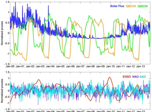
(Xj) are used here to parameterize the ozone variations on non-seasonal timescales.

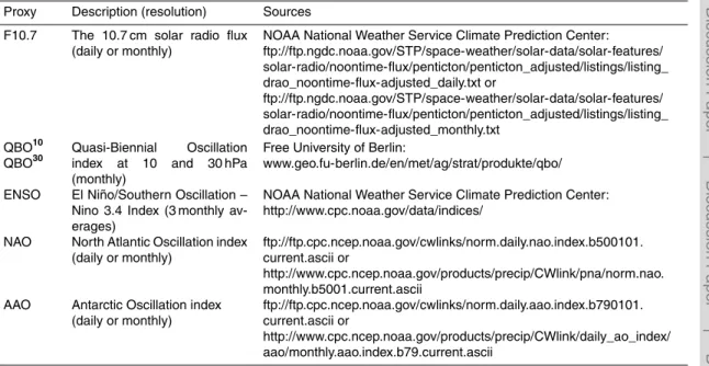
The chosen proxies areF_10.7, QBO10, QBO30, ENSO, NAO/AAO, the first three being the most commonly used (“standard”) proxies to describe the natural ozone variability, i.e. the solar radio flux at 10.7 cm and the quasi-biennial oscillation (QBO) which is represented by two orthogonal zonal components of the equatorial stratospheric wind

5

measured at 10 and 30 hPa, respectively (e.g. Randel and Wu, 2007). The three other proxies, ENSO, NAO and AAO, are used to account for other important fluctuating dy-namical features: the El Niño/Southern Oscillation, the North Atlantic Oscillation and the Antarctic Oscillation, respectively. Table 1 lists the selected proxies, their sources and their resolutions. The time series of these proxies normalized over the 2000–2013

10

period following Eq. (2) are shown in Fig. 3a and b and they are shortly described hereafter:

– Solar flux: over the period 2008–2013, the radio solar flux increases from about 65 units in 2008 to 180 units in 2013 and is characterized by a specific daily “fingerprint” (see Fig. 3a). Note that because the period of IASI observations do

15

not cover a full 11 year solar cycle, it could affect the determination of the trend in the regression procedure. The difficulty in discriminating both components is a known problem for such multivariate regression: it feeds into their uncertainties and it can lead to biases in the coefficients determination (e.g. Soukharev et al., 2006).

20

– QBO terms: the QBO of the equatorial winds is a main component of the dy-namics of the tropical stratosphere (Chipperfield et al., 1994, 2003; Randel and Wu, 1996, 2007; Logan et al., 2003; Tian et al., 2006; Fadnavis and Beig, 2009; Hauchecorne et al., 2010). It strongly influences the distributions of stratospheric O₃ propagating alternatively westerly and easterly with a mean period of 28 to

25

(10)

re-ACPD

15, 27575–27625, 2015

C. Wespes et al.

Title Page

Tables Figures

◭ ◮

Back Close

Full Screen / Esc

Discussion

P

a

per

|

Discussion

P

a

per

|

Discussion

P

a

per

|

Discussion

P

a

per

|

lationship between the QBO periodic oscillations in the upper and in the lower stratosphere, orthogonal QBO time series at 10 hPa (Fig. 3a; orange) and 30 hPa (Fig. 3a; green) based on observed stratospheric winds at Singapore have been considered here (Randel and Wu, 1996; Hood and Soukharev, 2006).

– NAO, AAO and ENSO: these proxies describe important dynamical features which

5

affect ozone distributions in the troposphere and the lower stratosphere (e.g. Weiss et al., 2001; Frossard et al., 2013; Rieder et al., 2013; and references therein). The daily or 3 monthly average indexes used to parameterize these fluc-tuations are shown in Fig. 3b. The NAO and AAO indexes are used for the N.H. and the S.H. (Southern Hemisphere), respectively (both are used for the

equato-10

rial band). These proxies have been included in the statistical model for complete-ness even if they are expected to only have a weak apparent contribution to the IASI ozone time series due to their large spatial variability in a zonal band (e.g. Frossard et al., 2013; Rieder et al., 2013).

– Effective equivalent stratospheric chlorine (EESC): the EESC is a common proxy

15

used for describing the influence of the ODS in O₃ variations. However, because the IASI time series starts several years after the turnaround for the ozone hole recovery in 1996/1997 (WMO, 2010), their influence is not represented by a ded-icated proxy but is rather accounted for by the linear trend term.

Even if some of the above proxies are only specific to processes occurring in the

20

stratosphere, we adopt the same approach (geophysical variables, model and regres-sion procedure) for adjusting the IASI O₃ time series in the troposphere. This proves useful in particular to account for the stratospheric contribution to the tropospheric layer (∼30–60 %; see Sect. 2 and Supplement, Fig. S3) due to stratosphere–troposphere

exchanges (STE) and to the fact that this tropospheric layer is not perfectly

decorre-25

(11)

ACPD

15, 27575–27625, 2015

C. Wespes et al.

Title Page

Tables Figures

◭ ◮

Back Close

Full Screen / Esc

Discussion

P

a

per

|

Discussion

P

a

per

|

Discussion

P

a

per

|

Discussion

P

a

per

|

account in the model in the harmonic and the linear trend terms of the Eq. (1) (e.g. Lo-gan et al., 2012). Including harmonic terms having 4 and 3 month periods in the model has been tested to describe O₃ dependency on shorter scales (e.g. Gebhardt et al., 2014), but this did not improved the results in terms of residuals and uncertainty of correlation coefficients.

5

3.3 Iterative backward variable selection

Similarly to previous studies (e.g. Steinbrecht et al., 2004; Mäder et al., 2007, 2010; Knibbe et al., 2014), we perform an iterative stepwise backward elimination approach, based onp values of the regression coefficients for the rejection, to select the most relevant combination of the above described regression variables (harmonic, linear

10

and explanatory) to fit the observations. The minimum p value for a regression term to be removed (exit tolerance) is set at 0.05, which corresponds to a significance of 95 %. The initial model which includes all regression variables is fitted first. Then, at each iteration, the variables characterized bypvalues larger than 5 % are rejected. At the end of the iterative process, the remaining terms are considered to have significant

15

influence on the measured O₃ variability while the rejected variables are considered to be non-significant. The correction accounting for the autocorrelation in the noise residual is then applied to give more confidence in the coefficients determination.

4 Ozone variations observed by IASI

In this section, we first examine the ozone variations in IASI time series during 2008–

20

(12)

ACPD

15, 27575–27625, 2015

C. Wespes et al.

Title Page

Tables Figures

◭ ◮

Back Close

Full Screen / Esc

Discussion

P

a

per

|

Discussion

P

a

per

|

Discussion

P

a

per

|

Discussion

P

a

per

|

4.1 O3time series from IASI

Figure 4a shows the time development of daily O₃ number density over the entire alti-tude range of the retrieved profiles based on daily medians. The time series cover the six years of available IASI observations and are separated in three 20◦ _{latitude belts:}

30–50◦N (top panel), 10–10◦S (middle panel) and 30–50◦S (bottom panel). The

fig-5

ure shows the well-known seasonal cycle at mid-latitudes in the troposphere and the stratosphere with maxima observed in spring-summer and in winter-spring, respec-tively, and a strong stability of ozone layers with time in the equatorial belt. At high latitudes of both hemispheres, the high ozone concentrations and the large amplitude of the seasonal cycle observed in LS and UTLS are mainly the consequence of the

10

large-scale downward poleward Brewer–Dobson circulation which is prominent in later winter below 25 km.

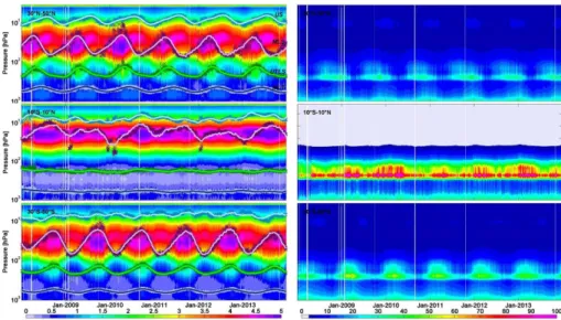
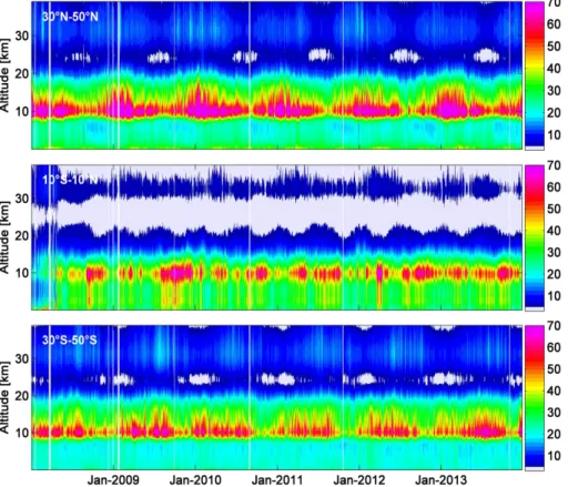
Figure 4b presents the estimated statistical uncertainty on the O₃profiles retrieved from FORLI. This total error depends on the latitude and the season, reflecting, amongst other, the influence of signal intensity, of interfering water lines and of thermal

15

contrast under certain conditions (e.g. temperature inversion, high thermal contrast at the surface). It usually ranges between 10 and 30 % in the troposphere and in the UTLS (Upper Troposphere–Lower Stratosphere), except in the equatorial belt due to the low O₃amounts (see Fig. 4a) which leads to larger relative errors. The retrieval errors are usually less than 5 % in the stratosphere.

20

The relative variability (given as the standard deviation) of the daily median O₃time series presented in Fig. 4a is shown in Fig. 5, as a function of time and altitude. It is worth noting that, except in the UTLS over the equatorial band, the standard deviation is larger than the estimated retrieval errors of the FORLI-O₃data (∼25 vs.∼15 % and ∼10 vs. ∼5 %, on average over the troposphere and the stratosphere, respectively),

25

(13)

ACPD

15, 27575–27625, 2015

C. Wespes et al.

Title Page

Tables Figures

◭ ◮

Back Close

Full Screen / Esc

Discussion

P

a

per

|

Discussion

P

a

per

|

Discussion

P

a

per

|

Discussion

P

a

per

|

play an important role. The largest values (>70 % principally in the northern latitudes during winter) are measured around 9–15 km altitude. They highlight the influence of tropopause height variations and the STE processes. In the stratosphere, the variability is always lower than 20 % and becomes negligible in the equatorial region. Interestingly, the lowest troposphere of the N.H. (below 700 hPa;<4 km) is marked by an increase in

5

both O₃ concentrations (Fig. 4a) and standard deviations (between∼30 and∼45 %)

in spring-summer. This likely indicates a photochemical production of O₃ associated with anthropogenic precursor emissions (e.g. Logan et al., 1985; Dufour et al., 2010; Safieddine et al., 2013).

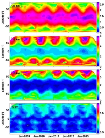
The zonal representation of the O₃variability seen by IASI is given in Fig. 6. It shows

10

the daily number density at altitude levels corresponding to maximum of sensitivity in the four analyzed layers in most of the cases (600 hPa –∼6 km; 240 hPa – ∼10 km;

80 hPa – ∼20 km; 6 hPa – ∼35 km) (Sect. 2). The top panel (∼35 km) reflects well

the photochemical O₃ production by sunlight with the highest values in the equato-rial belt during the summer (∼3×1012molecules cm−3). The middle panels (∼20 and

15

∼10 km) shows the transport of ozone rich-air to high latitudes in late winter (up to ∼6×1012molecules cm−3in the N.H.) which is induced by the Brewer–Dobson

circu-lation. The fact that the patterns are similar in ∼10 km mainly reflects the low

sen-sitivity of IASI to that level compared to the others. Finally, the lower panel (∼6 km)

presents high O₃levels in spring at high latitudes (∼1.4×1012molecules cm−3in the

20

N.H.), which likely reflects both the STE processes and the contribution from the strato-sphere due to the medium IASI sensitivity to that layer (cfr. Sect. 2 and Supplement), and a shift from high to middle latitudes in summer which could be attributed to an-thropogenic O₃production. The MLT panel also reflects the seasonal oscillation of the Inter-Tropical Convergence Zone (ITCZ) around the Equator and the large fire activity

25

(14)

ACPD

15, 27575–27625, 2015

C. Wespes et al.

Title Page

Tables Figures

◭ ◮

Back Close

Full Screen / Esc

Discussion

P

a

per

|

Discussion

P

a

per

|

Discussion

P

a

per

|

Discussion

P

a

per

|

4.2 Multivariate regression results: seasonal and explanatory variables

Figure 4a shows superimposed on the time series of the IASI ozone concentration profile, those of the partial columns (dots) for the 4 layers (color scale). The adjusted daily time series to these columns with the regression model defined by Eq. (1) is also overlaid and shown by colored lines. The model reasonably well represents the ozone

5

variations in the four layers, with, as illustrated for three latitude bands, good coeffi-cient correlations (e.g.RMLT=0.94;RUTLS=0.91; RMLT=0.90 andRUS=0.91 for the 30–50◦_{N band) and low residuals (}_<_{8 %) in all cases. However, note that the fit fails}

to reproduce the highest ozone values (>5×1012molecules cm−3) above the seasonal

maxima for 30–50◦_{N latitude band, especially in the MLS during the springs 2009 and}

10

2010. This could be associated with occasional downward transport of upper atmo-spheric NO_x-rich air occurring in winter and spring at high latitudes (Brohede et al., 2008) following the strong subsidence within the intense Arctic vortex in 2009–2010 (Pitts et al., 2011).

Figure 7 displays the annual cycle averaged over 6 years recorded by IASI (dots) for

15

the studied layers and bands, as well as that from the fit of the daily O₃columns (lines). The regression model follows perfectly the O₃variations in terms of timing of O₃ max-ima and of amplitude of the cycle. The fit is generally characterized by low residuals (<10 %) and good correlation coefficients (0.70–0.95), which indicates that the regres-sion model is suitable to describe the zonal variations. Exception is found over the

20

Southern latitudes (residual up to 15 % andR down to 0.61) probably because of the variation induced by the ozone hole formation which is not parameterized in the regres-sion model, and because of the low temporal sampling of daytime IASI measurements in this region.

From Fig. 7, the following general patterns in the O₃seasonal cycle can be isolated

25

from the zonally averaged IASI datasets:

(15)

ACPD

15, 27575–27625, 2015

C. Wespes et al.

Title Page

Tables Figures

◭ ◮

Back Close

Full Screen / Esc

Discussion

P

a

per

|

Discussion

P

a

per

|

Discussion

P

a

per

|

Discussion

P

a

per

|

to the averaged O₃ values. The largest amplitude in the annual cycle is found in the N.H. between 30 and 50◦_{N where O}

3peaks in July after the highest solar el-evation (in June) following a progressive buildup during spring-summer. In agree-ment with FTIR observations (e.g. Steinbrecht et al., 2006; Vigouroux et al., 2008), a shift of the O₃ maximum from spring (March–April) to late summer (August–

5

September) is found as one moves from high to low latitudes in the N.H. In the S.H., the general shape of the annual cycle which shows a peak in October– November before the highest solar elevation (in December), results from loss mechanisms depending on annual cycle of temperatures and other trace gases. Other effects such as changing Brewer–Dobson circulation, light absorption and

10

tropical stratopause oscillations may also considerably impact on the cycle in this layer (Brasseur and Solomon, 1984; Schneider et al., 2005).

2. In the lower stratosphere (MLS and UTLS, middle panels), the pronounced am-plitudes of the annual cycle is dominated by the influence of the Brewer Dob-son circulation with the highest O₃ values observed over polar regions (reaching

15

∼6×1018molecules cm−2 on average vs.∼2×1018molecules cm−2 on average

in the equatorial belt). The maximum is shifted from late winter at high latitudes to spring at lower latitudes.

3. In MLT (bottom panel), we clearly see a large hemispheric difference with the highest values over the N.H. (also in UTLS). Maxima are observed in spring,

re-20

flecting more effective STE processes. A particularly broad maximum from spring to late summer is observed in the 30–50◦N band. It probably points to anthro-pogenic production of O₃. This has been further investigated in the Supplement through MOZART4-IASI comparison by using constant anthropogenic emissions in the model settings (see Fig. S1). The results show clear differences between

25

(16)

ACPD

15, 27575–27625, 2015

C. Wespes et al.

Title Page

Tables Figures

◭ ◮

Back Close

Full Screen / Esc

Discussion

P

a

per

|

Discussion

P

a

per

|

Discussion

P

a

per

|

Discussion

P

a

per

|

Figure 8 presents all the fitted regression parameters included in Eq. (1) (Sect. 3) in the four layers as a function of latitude. The uncertainty in the 95 % confidence limits which accounts for the autocorrelation in the noise residual is given by error bars. The constant term (Fig. 8a) is found to be statistically significant (uncertainty

<10 %) in all cases. It captures the two ozone maxima in the stratosphere: one over

5

the Northern Polar regions in the MLS and one at equatorial latitudes in the US (∼

4.5×1018molecules cm−2), the important decrease of O3 in the lower stratospheric layers (UTLS and MLS) moving from high to equatorial latitudes, and the weak negative and strong positive gradients in the Northern MLT and in the US, respectively. The sum of the constant terms of the four layers varies between 7.50×1018 (equatorial region)

10

and 9.50×1018molecules cm−2(polar regions) and is similar to the one of the fitted total

column (relative differences<3.5 %) (red line). When analyzing the constant terms, it is worth keeping in mind that FORLI-O₃profiles are biased high in the UTLS region by

∼10–15 % in the mid-latitudes and in the tropics (Dufour et al., 2012; Gazeaux et al.,

2012). The representativeness of the 20◦ _{zonal averages in terms of spatial variability}

15

has been examined by fitting the IASI time series for specific locations in the N.H. (results shown with stars in Fig. 8a): the constant terms are found to be consistent, within their uncertainties, with those averaged per latitude bands in all cases. Over the polar region where O₃ shows a large natural variability, the regression coefficient is characterized by a large uncertainty.

20

The regression coefficients for other variables (harmonic and proxy terms) which are retained in the regression model by the stepwise elimination procedure are shown in Fig. 8b. They are scaled by the fitted constant term and the error bars represent the uncertainty in the 95 % confidence limits accounting for the autocorrelation in the noise residual. We find that:

25

1. The annual harmonic term (upper left) is the main driver of the O₃variability and largely dominates (scaleda₁+b₁around±40 %) over the semi-annual one (upper

right; scaleda₂+b₂ around±15 %). In UTLS and MLS, its amplitude decreases

(17)

ACPD

15, 27575–27625, 2015

C. Wespes et al.

Title Page

Tables Figures

◭ ◮

Back Close

Full Screen / Esc

Discussion

P

a

per

|

Discussion

P

a

per

|

Discussion

P

a

per

|

Discussion

P

a

per

|

circulation (cfr. Fig. 6 and Fig. 7) and the sign of the coefficient accounts for the winter-spring maxima in both hemispheres (negative values in the S.H. and pos-itive ones in the N.H). In the US, they vary only slightly (around −5 to 5 %) and

account for the weak summer maximum.

2. The QBO and solar flux proxies are generally minor (scaled coefficients<10 %)

5

and they are even statistically non-significant contributors to O₃variations after ac-counting for the autocorrelation in the noise residual, except for the UTLS in equa-torial region (scaled coefficients of 10–15 %) where they are important drivers of O₃ variations (e.g. Logan et al., 2003; Steinbrecht et al., 2006b; Soukharev and Hood, 2006; Fadnavis and Beig, 2009) Previous studies have indeed

sup-10

ported the solar influence on the lower stratospheric equatorial dynamics (e.g. Soukharev and Hood, 2006; McCormack et al., 2007). Note that the QBO30proxy (data not shown) has negative coefficients for the mid-latitudes, which is in line with Frossard et al. (2013).

3. The contributions described by the ENSO and NAO/AAO proxies are generally

15

very weak, with scaled coefficients lower than 5 %, and, in many cases, even not statistically significant when taking into account the correlation in the noise residu-als. Despite of this, it is worth pointing out that their effects to the O₃variations are in agreement with previous studies, which have shown large regions of negative coefficients for NAO North of 40◦_{N, and large regions of positive and negative}

20

coefficient estimates for ENSO, North of 30◦_{N and South of 30}◦_{S, respectively}

(Rieder et al., 2013; Frossard et al., 2013).

Finally, we see in Fig. 8b, large uncertainties associated with the regression coeffi-cients in UTLS in comparison with other layers, and in polar regions in comparisons with other bands. We interpret this as an effect from the high natural variability of O₃

25

(18)

ACPD

15, 27575–27625, 2015

C. Wespes et al.

Title Page

Tables Figures

◭ ◮

Back Close

Full Screen / Esc

Discussion

P

a

per

|

Discussion

P

a

per

|

Discussion

P

a

per

|

Discussion

P

a

per

|

4.3 Multivariate regression results: trend over 2008–2013

An additional goal of the multivariate regression method applied to the IASI O₃ time series is to determine the annual trend term and its associated uncertainty. Despite the fact that more than 10 years of observations, corresponding to the large scale of solar cycle, is usually required to perform such a trend analysis, we could argue that

5

statistically relevant trends could possibly be derived from the first six years of IASI observations, owing to the high spatio-temporal frequency (daily) of IASI global ob-servations, to the daily “fingerprint” in the solar flux (see Fig. 3a), possibly making it distinguishable from a linear trend, and to its weak contribution to O₃ variations (see Sect. 4.2 and references therein). To verify the specific advantage of IASI in terms of

10

frequency sampling, we compare, in the subsections below, the statistical relevance of the trends when retrieved from the monthly averaged IASI datasets vs. the daily averages as above, in the 20◦_{zonal bands.}

4.3.1 Regressions applied on daily vs. monthly averages

Figure 9 (top) provides, as an example for the 30–50◦_{S latitude band, the 6 year time}

15

series of the IASI O₃partial column in the US (dark blue), for daily averages (left panels) vs monthly averages (right panels), along with the results from the regression proce-dure (light blue). Note that either daily or monthly F10.7, NAO and AAO proxies (see Table 1) are used depending on the frequency of the IASI O₃averages to be adjusted. The middle panels provide the deseasonalised IASI and fitted time series as well as

20

the residuals (red curves). The fitted signal in DU of each proxy is shown on the bottom panels. The O₃time series and the solar flux signal resulting from the adjustment with-out the linear term trend in the regression model are also represented (orange lines in middle and bottom panels, respectively). When it is not included in the regression model, the linear trend term is not compensated by the solar flux term in the daily

aver-25

(19)

with-ACPD

15, 27575–27625, 2015

C. Wespes et al.

Title Page

Tables Figures

◭ ◮

Back Close

Full Screen / Esc

Discussion

P

a

per

|

Discussion

P

a

per

|

Discussion

P

a

per

|

Discussion

P

a

per

|

out vs. 60 % with the linear term). In this example, the linear and solar flux terms are even not simultaneously retained in the iterative stepwise backward procedure when applied on the monthly averages while they are when applied on daily averages. This effective co-linearity of the linear and the monthly solar flux terms translates to a large uncertainty for the trend coefficient in monthly data and leads, in this example, to a not

5

statistically significant linear term of 1.21±1.30 DU yr−1 when derived from monthly

averages vs. a significant trend of 1.74±0.77 DU yr−1from daily averages.

This brings us to the important conclusion that, thanks to the unprecedented sam-pling of IASI, apparent trends can be detected in FORLI-O₃time series even on a short period of measurements. This supports the need for regular and high frequency

mea-10

surements for observing ozone variations underlined in other studies (e.g. Saunois et al., 2012). The O₃ trends from the daily averages of IASI measurements are dis-cussed and compared with results from the monthly averages in the subsection below.

4.3.2 O3trends from daily averages

Table 2 summarizes the trends and their uncertainties in the 95 % confidence limit,

cal-15

culated for each 20◦zonal band and for the 4 partial and the total columns. For the sake of comparison, the trends are reported for both the daily (top values) and the monthly (bottom values) averages, and their uncertainties account for the auto-correlation in the noise residuals considering a time lag of 1 day or 1 month, respectively. We show that the daily and monthly trends fall within each other uncertainties but that the trends

20

in monthly averages are shown to be mostly non-significant in comparison with those from daily averages for the reasons discussed above (Sect. 4.3.1). Table 3 summarizes the trends in the daily averages for two 3 month periods: June–July–August (JJA) and December–January–February (DJF).

From Tables 2 and 3, we observe very different trends according to the latitude and

25

(20)

ACPD

15, 27575–27625, 2015

C. Wespes et al.

Title Page

Tables Figures

◭ ◮

Back Close

Full Screen / Esc

Discussion

P

a

per

|

Discussion

P

a

per

|

Discussion

P

a

per

|

Discussion

P

a

per

|

data (Weatherhead and Anderson, 2006; Knibbe et al., 2014) or from ground-based measurements (Vigouroux et al., 2008) over longer time periods. The non-significant trends calculated for the mid- and low latitudes of the N.H. are also in agreement with previous studies (Reinsel et al., 2005; Andersen and Knudsen, 2006; Vigouroux et al., 2008). Regarding the individual layers, we find the following:

5

1. In the US, significant positive trends are observed in both hemispheres from the daily medians, particularly over the mid- and high latitudes of the both hemi-spheres (e.g. 1.74_±0.77 DU yr−1_{in the 30–50}◦_{S band, i.e., 12 % decade}−1_{) where} the change in ozone trends before and after the turnaround in 1997 is the highest (Kÿrola et al., 2013; Laine et al., 2014). Positive trends in the US are in

agree-10

ment with many previous observations if one considers the fact that the period covered by IASI is later than those reported in previous studies and that the re-covery rate seems to heighten since the beginning of the turnaround (Knibbe et al. (2014) reports a factor of two in the recovery rate between 1997–2010 and 2001–2010), and they could indicate a leveling off of the negative trends that

15

was existing since the second half of the 1990’s (e.g. WMO 2006, 2011; Ran-del and Wu, 2007; Vigouroux et al., 2008; Steinbrecht et al., 2009; Jones et al., 2009; McLinden et al., 2009; Laine et al., 2014; Nair et al., 2014). The causes of this “turnaround” remain, however, uncertain. If the compensating impact of de-creasing chlorine in recent years and maximum solar cycle (over 2011–2012 in

20

the period studied here) is probably part of the answer (e.g. Steinbrecht et al., 2004), the effects of changing stratospheric temperatures and Brewer–Dobson circulation (Salby et al., 2002; Reinsel et al., 2005; Dhomse et al., 2006; Manney et al., 2006) could also contribute and should be further investigated. The long-lasting cold winter/spring 2011 in the Arctic conducting to unprecedented ozone

25

loss (Manney et al., 2011), could explain the non-significant trend in the 70–90◦_N

(21)

ACPD

15, 27575–27625, 2015

C. Wespes et al.

Title Page

Tables Figures

◭ ◮

Back Close

Full Screen / Esc

Discussion

P

a

per

|

Discussion

P

a

per

|

Discussion

P

a

per

|

Discussion

P

a

per

|

trends in winter. A non-significant trend is also calculated for the 70–90◦_{S band}

in spring (data not shown). This could indicate the strong influence of changing stratospheric temperatures on ozone depletion from year to year (e.g. Dhomse et al., 2006), leading to larger uncertainties in our trends estimations and larger fitting residuals (see Sect. 4.2) due to the fact that the stratospheric temperature

5

is not taken into account as an explanatory variable in the model.

2. In the MLS, one can see that, except in the high latitude bands, the trends are either non-significant or significantly negative. This is in agreement with the trend analysis of Jones et al. (2009) for the 20–25 km altitude range over the 1997– 2008 period, as well as with other studies at N.H. latitudes, which investigated

10

O₃ changes in the 18–25 km range between 1996 and 2005 (Miller et al., 2006; Yang et al., 2006; Kivi et al., 2007). The results derived separately for summer and winter in Table 3 are also in line with those of Kivi et al. (2007) which reported contrasted trends in the Arctic MLS depending on season.

3. In the UTLS, negative trends are calculated in the tropics and significant

posi-15

tive trends are found in the mid- and high latitudes of N.H., these latter falling within the uncertainties of those reported by Kivi et al. (2007) for the tropopause-150 hPa layer between 1996 and 2003. The large positive trends calculated at Northern latitudes (e.g. 1.28±0.82 DU year−1in the 70–90◦N band) contribute for ∼30 % to the positive trend for the total column. This result is in agreement with

20

Yang et al. (2006) which reported that UTLS contributes 50 % to positive trends for the total columns measured in the mid-latitudes of the N.H. from ozonesondes. In that study, these positive trends were linked to changes in atmospheric dynam-ics either related to natural variability induced by potential vorticity and tropopause height variations or related to anthropogenic climate change. Hence, the apparent

25

(22)

ACPD

15, 27575–27625, 2015

C. Wespes et al.

Title Page

Tables Figures

◭ ◮

Back Close

Full Screen / Esc

Discussion

P

a

per

|

Discussion

P

a

per

|

Discussion

P

a

per

|

Discussion

P

a

per

|

2008; Nair et al., 2014). It is worth to keep in mind that these effects are not in-dependently accounted for in the regression model. Previous studies reported, however, that dynamical and chemical processes are physically coupled in the atmosphere, making difficult to define unambiguously such drivers in a statistical model (e.g. Mäder et al., 2007; Harris et al., 2008). On a seasonal basis (see

Ta-5

ble 3), the trends seen by IASI at Northern latitudes in summer are all significantly positive and increasing towards the pole. Note that the trends in upper layers may contribute to the ones calculated in UTLS due to the medium IASI sensitivity to that layer (cfr. Sect. 2).

4. In the MLT, most of the trends are significantly negative (Tables 2 and 3). The

10

non-significant trends in polar regions could be partly related to the lack of IASI sensitivity to tropospheric O₃ (see Sect. 2, Fig. 2). On a seasonal basis, we see that the negative trends are more pronounced during the JJA period (around

−0.25±0.10 DU yr−1) for all bands except between 30◦N and 10◦S. In the N.H.,

these results tend to confirm the leveling offof tropospheric ozone observed in

re-15

cent years during the summer months (Logan et al., 2012). This trend, however, remains difficult to interpret because it could be linked to a variety of processes including most importantly: the decline of anthropogenic emissions of ozone pre-cursors, the increase of UV-induced O₃destruction in the troposphere and STE processes (Isaksen et al., 2005; Logan et al., 2012; Parrish et al., 2012; Hess and

20

Zbinden, 2013). As for the upper layers, our results for the Arctic are in agreement with the findings of Kivi et al. (2007) which reported an increase of ozone in the ground-400 hPa layer in summer over the 1996–2003 period following changes in the Arctic Oscillation. It is also worth to keep in mind that due to medium sensitiv-ity of IASI to the troposphere, ozone variations in upper layers may largely impact

25

(23)

ACPD

15, 27575–27625, 2015

C. Wespes et al.

Title Page

Tables Figures

◭ ◮

Back Close

Full Screen / Esc

Discussion

P

a

per

|

Discussion

P

a

per

|

Discussion

P

a

per

|

Discussion

P

a

per

|

4.3.3 O3trends from IASI vs. FTIR data

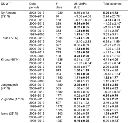
In order to validate the trends inferred from IASI in the US and in the total columns, we compare them with those obtained from ground-based FTIR measurements at sev-eral NDACC stations (Network for the Detection of Atmospheric Composition Change, available at http://www.ndsc.ncep.noaa.gov/data/data_tbl/) by using the same fitting

5

procedure and taking into account the autocorrelation in the noise residuals. A box of 1◦

×1◦centered on the stations has been used for the collocation criterion. The

regres-sion model is applied on the daily FTIR data for a series of time periods starting after the turnaround point (from 1998 for mid-latitude stations and from 2000 for polar sta-tions), as well as for the same periods as recently studied in Vigouroux et al. (2014) for

10

the sake of comparison. Note that because we are not interested here in validating the IASI columns which was achieved in previous papers (e.g. Dufour et al., 2014; Oetjen et al., 2014) but in validating the trends obtained from IASI, we did not correct biases between IASI and FTIR due to different vertical sensitivity and a priori information. The results are given in DU year−1in Table 4. We see large significant positive total column

15

trends from IASI at middle and polar stations (e.g. 5.26±4.72 DU yr−1at Ny-Alesund),

especially during spring and which are in agreement with the trends reported in Knibbe et al. (2014) for the 2001–2010 period. This trend is not obtained from the FTIR data for which trends are found to be mostly non-significant (even not retained in the stepwise elimination procedure in some cases) as reported in Vigouroux et al. (2014), except

20

at Jungfraujoch which shows a trend of 5.28±4.82 DU yr−1 over the 2008–2012

pe-riod. For the periods starting before 2000, we calculated from FTIR, in agreement with Vigouroux et al. (2014), a significantly negative trend at Ny-Alesund for the total column and significantly positive trends at polar stations for the US. In addition, we see from Table 4 a leveling offof O₃at polar stations in the US after 2003, as previously reported

25

(24)

ACPD

15, 27575–27625, 2015

C. Wespes et al.

Title Page

Tables Figures

◭ ◮

Back Close

Full Screen / Esc

Discussion

P

a

per

|

Discussion

P

a

per

|

Discussion

P

a

per

|

Discussion

P

a

per

|

trends are, however, non-significant and inferred only from few FTIR measurements (see Number of days column, Table 4).

From IASI, it is worth to point out that, in all cases, positive trends are calculated in the US (even if some are not significant) and that these trends are consistent with those calculated from FTIR data covering a _∼11 year period and starting after the

5

turnaround (e.g. at Thule; 1.24±1.09 DU yr−1from IASI for the period 2008–2013 vs.

1.42±0.78 DU yr−1from the FTIR over 2001–2012). This is illustrated for three stations

(Ny-Alesund, Thule and Kiruna) in Fig. 10 which compares the time series from IASI (2008–2013, in red) with those from FTIR covering periods starting after the turnaround (in blue). Their associated trends as well as the trend calculated from FTIR covering

10

the IASI period (in green) are also indicated.

The results obtained for trends inferred from IASI vs. FTIR tend to confirm the con-clusion drawn in Sects. 4.3.1 and 4.3.2, that the temporal sampling of IASI provides good confidence in the determination of the trends even on periods shorter than those usually required from other observational means.

15

5 Summary and conclusions

In this study, we have analyzed 6 years of IASI O₃ profile measurements as well as the total O₃ columns based on the profile. Four layers have been defined following the ability of IASI to provide reasonably independent information on the ozone partial columns: the mid-lower troposphere (MLT), the upper troposphere – lower stratosphere

20

(UTLS), the mid-lower stratosphere (MLS) and the upper stratosphere (US). Based on daily values of these four partial or of the total columns in 20◦ zonal averages, we have demonstrated the capability of IASI for capturing large scale ozone variability (seasonal cycles and trends) in these different layers. We have presented daytime vertical and latitudinal distributions for O₃ as well as their evolution with time and we

25

(25)

ACPD

15, 27575–27625, 2015

C. Wespes et al.

Title Page

Tables Figures

◭ ◮

Back Close

Full Screen / Esc

Discussion

P

a

per

|

Discussion

P

a

per

|

Discussion

P

a

per

|

Discussion

P

a

per

|

at equatorial region in the US, while they reflect the impact of the Brewer–Dobson circulation with maximum in winter-spring at mid- and high latitude in the MLS and in the troposphere. The effect of the photochemical production of O₃from anthropogenic precursor emissions was also observed in the troposphere with a shift in the timing of the maximum from spring to summer in the mid-latitudes of the N.H.

5

The dynamical and chemical contributions contained in the daily time development of IASI O₃ have been analyzed by fitting the time series in each layer and for the total column with a set of parameterized geophysical variables, a constant factor and a linear trend term. The model was shown to perform well in term of residuals (<10 %), correlation coefficients (between 0.70 and 0.99) and statistical uncertainties (<7 %) for

10

each fitted proxies. The annual harmonic terms (seasonal behavior) were found to be largely dominant in all layers but the US, with fitted amplitudes decreasing from high to low latitudes in agreement with the Brewer–Dobson circulation. The QBO and solar flux terms were calculated to be important only in the equatorial region, while other dynamical proxies accounted for in the regression (ENSO, NAO, AAO) were found

15

negligible.

Despite the short time period of available IASI dataset used in this study (2008–2013) and the potential ambiguity between the solar and the linear trend terms, statistically significant trends were derived from the six first years of daily O₃partial columns mea-surements (on the contrary to monthly averages which lead to mostly non-significant

20

trends). This result which was strengthened from comparisons with the regression ap-plied on local FTIR measurements, is remarkable as it demonstrates the added value of IASI exceptional frequency sampling for monitoring medium to long-term changes in global ozone concentrations. We found two important apparent trends:

1. Significant positive trends in the upper stratosphere, especially at high latitudes in

25

both hemispheres (e.g. 1.74±0.77 DU yr−1 in the 30–50◦S band), which is

(26)

ACPD

15, 27575–27625, 2015

C. Wespes et al.

Title Page

Tables Figures

◭ ◮

Back Close

Full Screen / Esc

Discussion

P

a

per

|

Discussion

P

a

per

|

Discussion

P

a

per

|

Discussion

P

a

per

|

trends calculated for some local stations are in line with those calculated from FTIR measurements after the turnaround.

2. Negative trends in the troposphere at mid- and high Northern latitudes, especially during summer (e.g.−0.26±0.11 DU yr−1in the 30–50◦N band) which are in link

with the decline of ozone precursor emissions.

5

To confirm the above findings beyond the 6 first years of IASI measurements and to better disentangle the effects of dynamical changes, of the 11 year solar cycle and of the equivalent effective stratospheric chlorine (EESC) decline on the O₃ time series, further years of IASI observations will be required, and more complete fitting proce-dures (including, among others, proxies to account for the decadal trend in the EESC,

10

ozone hole formation) will have to be explored. This will be achievable with the long term homogeneous records obtained by merging measurements from the three suc-cessive IASI instruments on MetOp-A (2006); -B (2012) and -C (2018), and by IASI successor on EPS-SG after 2021 (Clerbaux and Crevoisier, 2013; Crevoisier, 2014).

The Supplement related to this article is available online at

15

doi:10.5194/acpd-15-27575-2015-supplement.

Acknowledgements. IASI has been developed and built under the responsibility of the Centre National d’Etudes Spatiales (CNES, France). It is flown onboard the MetOp satellites as part of the EUMETSAT Polar System. The IASI L1 data are received through the EUMETCast near real time data distribution service. Ozone data used in this paper are freely available upon

20

request to the corresponding author. We acknowledge support from the O3-CCI project funded

by ESA and by the O3M-SAF project funded by EUMETSAT. P.-F. Coheur and C. Wespes are, respectively, Senior Research Associate and Postdoctoral Researcher with F.R.S.-FNRS. The research in Belgium was also funded by the Belgian State Federal Office for Scientific, Technical and Cultural Affairs and the European Space Agency (ESA Prodex IASI Flow and BO3MSAF).

25