Meson Loop Corrections to the NJL Model
Francisco Pe~na, M. Carolina Nemes,
Departamento de Fsica, Instituto de Ci^encias Exatas, Universidade Federal de Minas Gerais,
Belo Horizonte, CEP 30.161-970, C.P. 702, MG, Brazil
Alex H. Blin, and Brigitte Hiller
Departamento de Fsica, Universidade de Coimbra, P-3004-516 Coimbra, Portugal
Received 26 January, 1999
We present a symmetry preserving approach to 1=N (Nbeing the number of colors) corrections in
the Nambu-Jona-Lasinio model. This is achieved through an explicit 1=N expansion where N is
considered as a free parameter. Verication and use of the pertinent Ward identity to the next to leading order in 1=N is made in obtaining the Goldberger-Treiman relation. Although the present
results are not new, the approach may be useful for deriving higher (than one loop) corrections to the NJL model in a systematic way.
I Introduction
The Nambu-Jona-Lasinio (NJL) model [1] has proven to be a valuable tool for our understanding of pion chi-ral dynamics and sevechi-ral important aspects of chichi-ral symmetry in the domain of low energy hadron physics. Also of theoretical relevance is the fact that nonpertur-bative methods devised to treat the NJL model turned out to be adequate to study spontaneous symmetry breaking in conning quark models [2] and QCD [3].
This suggests that the study of chirally invariant nonperturbative approximations has considerable inter-est in its own right. In the context of the Nambu-Jona-Lasinio (NJL) [1] model the best known nonperturba-tive method is the one quark loop approximation. It has been applied to study numerous features of strong interaction physics at low energies (for recent reviews see [5]) with striking success. Much less work, how-ever, has been comparatively devoted to implementa-tions of higher order approximaimplementa-tions. Among these we can quote [6-10]. These approaches are based on a 1=N expansion, where N denotes the number of colors. As discussed in [10], symmetry properties of the system can be easily violated by an inappropriate choice of
di-agrams. Methods which preserve the symmetry proper-ties at higher orders deserve our special attention, refs. [9,10].
The purpose of this paper is to present a mathe-matical implementation of a 1=N expansion where N is considered as a free parameter. We make use of the Functional Integral Approach and show that a com-pletely systematic expansion can be constructed in such a way that itautomatically yields all necessary Feyn-man graphs to a given order in 1=N, being therefore self consistent. Our results coincide with those of refs.[9,10], which are symmetry preserving, to their calculation or-der. Higher order contributions can be computed in the present scheme. Moreover, we implement the calcula-tion of the pion decay constant within the very same approximation scheme and corrections to it are given by the same means and are on the same footing as cor-rections to the meson and fermion propagators.
II The Model
c
L= (i6@, ^m) + G2[( )
2+ ( i 5a )
2] ; a = 1;2;3 (1)
where a are the isospin matrices and ^m denotes the current quark mass, which we take to be equal in the u and d quark sectors. It is convenient to redene the strong coupling constant as g = GN in order to make the number of colors N explicit. It is helpful to repeat some well known techniques in the light of an expansion in terms of 1=N counting: We proceed to bosonize partially the Lagrangian, introducing auxiliary elds 'i with the quantum numbers of a scalar ^S and of pseudoscalar ^Paelds, in such a way that the new Lagrangian
L!L, 1 2g[^S,
g p
N ]2 ,
1 2g[^Pa
, g p
N i5a ]
2 (2)
has exactly the same dynamical content as the original one. One veries from the Euler-Lagrange equations of motion
L 'i
, L (@'i) = 0
(3)
that
^S = gp
N (4)
and
^Pa= g p
N ai5 (5)
and therefore all steps are exact. In terms of the new elds the Lagrangian reads
L=, 1 2g^S2
, 1 2g^P2
a + [i
6@, ^m + 1N(^S+ ^P
aai5)] : (6)
The expectation value of the scalar eld in vacuum < ^S >= p
Ns is nite. By shifting the scalar eld to a new eld with vanishing vacuum expectation value, < >= 0 one generates the constituent quark mass m, ,m + =
p
N =,^m + ^S= p
N. In terms of the new scalar eld and the pseudoscalar elds a one has
L= N( ,s
2 2g ) +
p N(sg)2
, 2 2g ,
2 a
2g + [i6@,m + 1 p
N ( + i5)] ; = a
Using functional integral methods, one introduces the generating function for the Green's functions
Z[; ;j
;ja] = N
0 Z
D D D
a D
ae
i(S+ + +j +j a a ) (8)
where S denotes the action and and are the source terms of the fermionic elds, and j, ja are the source terms of the scalar and pseudoscalar respectively. The normalization factorN
0is chosen such that
Z[0] = 1. The generating functional is therefore
Z[; ;j ;j
a] = N 0e i R d 4 xN(, s 2 2g ) Z
DDe R d 4 xN 0 [, 1 2g 2 , 1 2g 2 a ] ei R d 4 x p N[ s g ] Z F[; ]e
i R d 4 x(j +j a a ) (9)
with D = a
D a and
Z
F[; ] = Z
D D e i R d 4 x[
K + , ]
(10)
concerns the functional integration over the quark elds with K = i6@,m + 1
p
N ( + i5): (11)
With the usual shift
0= + K,1
0= + K,1 (12)
which leaves the integration measure invariant one obtains after integrating over the fermionic elds
Z[; ;j ;j
a] = e i
R d
4 x K
,1
eNTrlnKe i R d 4 x(j +j a a ) (13) where
Tr lnK = Tr ln(i6@,m) + i 1 X n=1 1 nN ,n 2 Tr[(i
6@,m)
,1( + i 5)]
n
The full generating functional is
Z[; ;j ;j
a] = N
Z
DDe i
R d
4 x K
,1
+j +j a
a
eS
eff (15)
where the eective action
Seff = p
NS1+ 12N 0S
2+ 1 3p
N S3+ 1
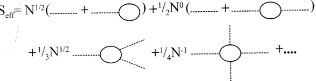
4N S4+ :::: (16)
shows explicitly how the the N-counting scheme enters in the dierent contributions in terms of n-point functions, Sn, see Fig. 1. One has
S1 = Z
d4
xsg,iTr[Y ] S2 =
, 1 g Z
d4x[2+ 2
a] + iTr[Y ] 2 S3 =
,iTr[Y ] 3 S4 = iTr[Y ]
4 (17)
with the denition Y = [(i 6 @,m)
,1( + i
5)]. To one quark loop level, n indicates the number of external mesonic elds, Sn corresponds to tree level contributions in terms of mesonic elds. In leading order of 1=N, one obtains the gap equation by calculating the stationary point of the eective action at < >= 0. The term S2 yields the two point functions, S3 and S4 the three and four point functions in leading order 1=N. To obtain the next-to-leading order corrections in a 1=N expansion of the gap equation and quark and meson propagators it is enough to consider terms up to S4. For decay processes involving three external mesonic lines, for instance, one would need to calculate S5 as well to describe the next-to-leading order corrections in 1=N.
Figure 1. The eective action with the explicit dependence on N of the several one-loop quark contributions. The dashed lines represent the meson elds. To the N
1=2 term contributes only the scalar meson; the propagator term, of order N
0,
stands for the pion and the sigma mesons; the three point function proportional toN
1=2involves either three scalars or one
scalar coupled to two pions; the four point function of order N
,1 stands for either all pions or all scalars or two pions and
two scalars.
calculation. For that one takes the unperturbed Lagrangian to be the one containing up to quadratic mesonic elds, and respective sources j
and j
a and treat perturbatively the higher eld powers, according to a perturbative expansion in 1=N, as
Z[ ; ; j
;j
a] = N
Z
D D e ,i
R d
4 x[ K
,1 ] e iS2 e iS2 e iSint e i R d 4 x[j +j a a ] (18) where S
int= 1 3p N
S 3+ 1
4N S 4+ :::: (19) e iS
int = 1 + i 3p N S 3+ i 4N S 4 , 1 18N S 3 S 3+
O(1=N 2)
:
(20)
The one point function in next to leading order in 1=N is obtained by deriving once with respect to the scalar meson source (the contribution from the pseudoscalar source vanishes) and requiring that the expectation value of the scalar eld vanishes in the new vacuum,
j
( x
1)
Z[ ;;j ;j a] j j=0 = iN Z
D D e ,i
R d
4 x[ K
,1 ] e iS 2 e iS 2 [1 + i
3p N
S 3+
:::](x 1) e i R d 4 x[j +j a a ] j j=0 =iN Z
D D e iS
2 e
iS 2[1 +
i 3p
N S
3+ :::](x
1) = 0 (21)
where the generic j stays for all sources. After performing all allowed contractions of the elds one obtains con-tributions up to the next to leading order in N to the one-point function, see also eq. 25 below. The subleading contribution is depicted in Fig. 2. At this stage it is interesting to compare the selfconsistency condition imposed by the gap equation on the vacuum expextation value of the scalar eld with the quark mass obtained from the quark propagator at next to leading order in 1=N. In leading order the constituent quark mass coincides with the vacuum expectation value of the scalar eld. In order to obtain the quark propagator one takes functional derivatives of Z[ ; ; j
;j
a] with respect to the fermionic sources
and , 2 (x 1) (x 2)
Z[ ;; j ;j a] j j=0 = ,N Z
D D 2 (x 1) (x 2)[ e ,i R d 4
x[ K ,1 ] e iS 2 e iS 2 e iSint] = ,N Z
By expanding [,iK ,1(x
1 ,x
2)] = (1 + Y ) ,1(i
6 @,m)
,1, in powers of Y up to order Y2, and expanding the exponential in Sintup to linear terms in Sint, one obtains
2 (x1)(x2)
Z[; ;j ;j
a] j
j=0 = ,iN
Z
DDe iS
2e
iS
2[1 + 1 p
N Y +N Y1 2](i
6@,m)
,1eiSint (23)
where the rst term in square brackets is the leading order inverse quark propagator, the term linear in Y multiplied by Sint(the S3 part of it) yields the Hartree contribution and the term in Y
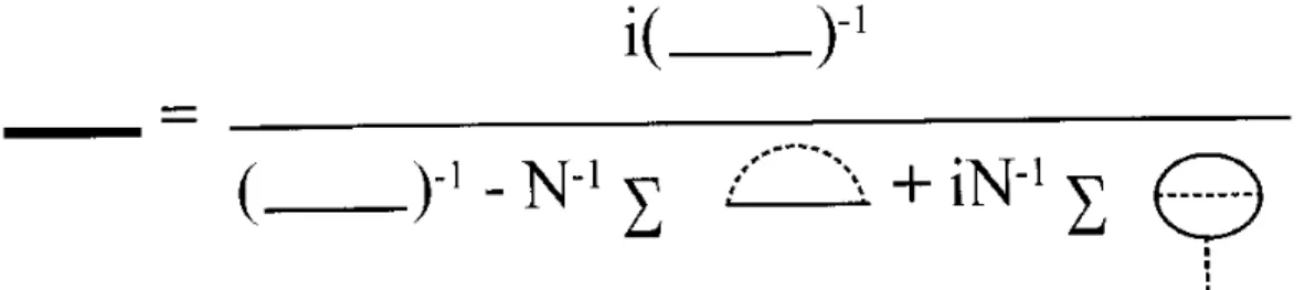
2 the Fock contribution to the next to leading order inverse quark propagator, see Fig. 3. The Fock terms renormalize the quark wave function and the Hartree terms contribute to the constant mass value in the gap equation, compare tadpole diagram of Fig. 3 with Fig. 2. Therefore the quark mass is precisely given by the gap equation when the fermion propagator has a pole, that is when eq. 21 is satised.
Figure 2. The next to leading order inN to the gap equation. The internal meson line stands for a pion or a sigma.
Figure 3. The quark propagator to the next to leading order in the 1=Nexpansion. The thin lines denote fermion propagators
in the dominant order, the dashed internal lines stand for pion and scalar insertions. The external line of the tadpole is a scalar.
The meson propagators are then obtained by deriving twice with respect to the mesonic sources. For instance the scalar propagator is
2 j
i(x 1)j
j(x 2)
Z[; ;j ;ja)
j j=0 = ,N
Z
DDe ,i
R d
4 x[K
,1 ]
eiS 2e
iS 2 [1 + i3p
N S3+ i4NS4 ,
1
18N S3S3](x2)(x1)e i
R d
4 x[j
+j
i
i ]
j j=0 =,N
Z
DDe iS
2e iS
2[1 + i 3p
N S3+ i4NS4 ,
1
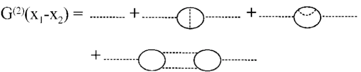
where i(x) stands for (x). The pion propagator is obtained with i(x) = i(x), the corresponding Feynman diagrams are shown in Fig. 4. For the explicit evaluation of the diagrams we use Pauli-Villars regularization with two covariant regulators, one for the quark loop momentum, , and one for the meson loop momentum. All needed integrals, Ii, i = 1;:::4, are given in the Appendix. We do not need to solve explicitly the meson loop integrals, since we are only interested in showing that the symmetry relations are preserved.
Figure 4. The meson propagator up to next to leading order in the 1=N expansion. In the present work we consider only
the pion propagator. The internal line stands in the upper two bubbles for a pion and a scalar and in the lower graph for a pion and a scalar insertion. The same types of diagrams emerge for the calculation of the weak pion decay constant, if one interprets the simple dashed line as well as one of the external lines in the bubble diagrams to be the axial vector current and the other the pseudoscalar meson.
Explicit evaluation of expression (21) yields for the gap equation
j(x1)
Z[;;j;j a]j
j=0=
m , ^m
G , G0(m), G(m), G(m) =0 (25)
with 0(m) = GG0(m) = 8mgI1the quark self energy of leading order and 1(m) = G(G(m)+G(m)) the quark loops with mesonic insertions, of next to leading order in 1=N. The equation
(m) = m = ^m + 0(m) + 1(m) (26)
must be solved selfconsistently for the samevalue of m, in all terms, as already pointed out in [10]. One has G(m) =,2ij
Z d4k (2)4
Z d4p (2)4
S(p)TrD[S(k)i5S(k,p)i5S(k)] (27)
with the quark propagator
S(k) = i6k,m (28)
and the inverse pion propagator in leading order S,1
(p) = ^m Gm + 4p2
I2(p) (29)
G(m) = ,24m
Z d4p (2)4
S(p)[
,I
2(0) + p 2I
3(0;p)] (30)
after summation over the isospin indices. This is the diagram of Fig. 2 with the internal meson line being a pion. For the quark loop with one scalar meson insertion one obtains
G(m) = 2 Z
d4k (2)4
Z d4p (2)4
S(p)TrD[S(k)S(k
,p)S(k)] (31)
where the inverse scalar propagator in leading order is
S,1
(p) = ^m
Gm + 4(p2 ,4m
2)I
2(p): (32)
One obtains
G(m) = 8m Z
d4p (2)4
S(p)[I2(0) + 2I2(p) + (4m 2
,p 2)I
3(0;p)]: (33)
Now we turn to the calculation of the pion propagator, using eq.24. We present the corrections to the selfenergy of the pion ij(q) =
P lP
ij
l (q) with
Pij 0 (q) =
ij(24I1 ,12q
2I 2(q
2)) (34)
being the lowest order contribution. The sum of all next to leading order terms 1
ij(q) contains the following terms Pij
1 (0) = 4 ij
Z d4p (2)4
S(p)
f2I 2(p
,q),q 2p2I
4(p;q;p + q)
g (35)
which is the rst bubble diagram in Fig. 4, with internal pion line;
Pij 2 (q) =
,24 ij
Z d4p (2)4
S(p) fI
2(p
,q) + I 2(0)
,2pqI 3(p;q)
,q 2I
3(0;q) + q 2p2I
4(0;p;q) g+
ijG
m (36)
which is the second bubble diagram in Fig. 4, with internal pion line;
Pij
3 (q) = 2 ij
Z d4p (2)4
S(p)
f4I 2(p
,q) + 2q 2(4m2
,p 2)I
4(q;p;p + q)
which is the rst bubble diagram in Fig. 4, with internal ;scalar meson line Pij
4 (q) = ,8
ij Z
d4p (2)4
S (p)
fI 2(p
,q),2I 2(0)
,2pqI 3(p;q)
,q 2I
3(0;q) ,(4m
2 ,p
2)I 3(0;p)
,q 2(4m2
,p 2)I
4(0;p;q) g+
ijG
m (38)
which is the second bubble diagram in Fig. 4, with internal scalar meson line;
Pij 5 =
,16 ij
Z d4p (2)4
S(p
,q) S(p)
f16m 2[I
2(p
,q),pqI 3(p;q)]
2
g (39)
which is the last diagram in Fig. 4, where the two internal meson lines are a pion and a scalar, respectively. To demonstrate the appearence of the Goldstone mode, we compare the quark selfenergy eq.26 to the pion selfenergy ij(q) and use the identity
S(p)
S (p) =
S(p)
, S(p) 16m2I
2(p
2) : (40)
In the chiral limit, ^m!0 one gets at q 2= 0
1(0) = 1
mG (41)
where 1(0) are all the contributions to the selfenergy of the pion except the leading one, and we use the notation ij(q) =
ij(q) Therefore the whole relation, including terms up to next to leadind order in N reads
= mG(0): (42)
The inverse pionic Green's function
S,1
(q) = G ,1
,(q) (43)
has therefore a zero at q2= 0 when the new gap equation = m is fullled, verifying the Goldstone theorem. See also discussion after eq. 60 below.
To calculate the weak decay constant fone incorporates in the model an axial current, connected to an external source. In this case the operator K will contain this current
K = i6@,m + 1p
N ( + i5+ p
N5aj 5a)
the Ward Identity relating the axialvector - pseudoscalar bubble A(q) to the pseudoscalar - pseudoscalar bubble (q),
A(q) = Aq = (m
, ^m)=G,m(q) (44)
with the notation Aij =
ijA(q) which holds at leading order in 1=N, holds at next to leading order too, which ensures that symmetry relations are preserved. The right hand side of this equation is just the inverse of the pion propagator multiplied by m. At next to leading order of 1=N there are several contributions to the bubbles A(q) and (q), as shown in Fig. 4.
Al(q) = Al(q)q
;l = 0;:::5 (45)
with A0(q) the leading order contribution
A0(q) = G0(m)
,4mN[2I 1
,q 2I
2(q)] (46)
and the remaining terms follow the same order as for Pl(q) in eqs. 35-39. The diagrams A1(q) and A2(q) correspond to the two distinct possibilities of having a pion propagator insertion in the quark loop, A3(q) and A4(q) are the equivalent diagrams for scalar propagator insertions and A5(q) denotes the diagram which couples the external elds to two o-shell mesonic propagators, a pion and a scalar. For diagram A1(q) we obtain
Aij 1(q) =
, X
l;l 0
Triljl 0
ll 0iN
Z d4p (2)4
Z d4k (2)4 f
S (p)TrDi5S(k ,q)i
6q 5
2 S(k)i5S(k ,p)i
5S(k
,p,q)g (47)
In order to derive the Ward identity (eq.44) we make use of the equality
6q =,(6k,6q,m) + (6k + m),2m (48)
in all Al(q) diagrams. We have then
A1(q) = ,2R
(q) ,mP
1(q) (49)
R ij(q) =
,4mN
iji Z
d4p (2)4
S (p)[I2(p
,q),pqI
3(p;q)] (50)
Aij 2(q) =
,2N X
l;l 0
Trill 0
jl;l 0i
Z d4k (2)4
Z d4p (2)4
S (p)
fTr
Di5S(k)iS(k ,q)i
6q 5
2 5S(k)i5S(k ,p)g = (G(q) + 6R
(q) ,mP
2(q))ij (51)
Aij 3(q) =
,2N iji
Z d4k (2)4
Z d4p (2)4
S (p) TrD
fS(k,q)i6q
5S(k)S(k ,p)i
5S(k
,p,q)g = (2R(q)
,mP
3(q))ij (52)
R
ij(q) = 4Nm ij
Z d4p (2)4
S(p)[I2(p) + (p q,q
2)I
3(p;q)] (53)
Aij 4(q) =
,2NTr iji
Z d4k (2)4i
Z d4p (2)4
S(p) TrD
fS(p)i 5S(k
,p)i 6q
2 5S(k)S(k ,p)g = (G(q) + 2R
(q) ,mP
4(q))ij (54)
Aij 5(q) = i
Z d4p (2)4
S(p)
S(p
,q)T il 1(p;q)T
jl
2 (p;q) (55)
where Til
1(p;q), (T 2)
jl(p;q) are the two quark triangles, coupling the axialvector, (pseudoscalar) to the two o-shell mesonic lines, respectively
Til
1(p;q) = 2N ili
Z d4k (2)4Tr
DS(k
,q)i6q
5S(k)i5S(k
Tjl
2 (p;q) = 2N jli
Z d4k (2)4Tr
Di5S(k)i5S(k
,q)S(k,p) (57)
The triangle Til
1(p;q) splits into the dierence of the two leading order inverse propagators S,1
(p) ,
S,1
(p
,q) and one gets
A5(q) = ,4(R
(q) + R(q)) ,mP
5(q): (58)
Summing up all contributions leads to
A = q X
i
Ai= G0(m) + G(m) + G(m) ,m
X i
Pi = (m, ^m)=G,m
X i
Pi (59)
using the result for the gap equation, eq.25. This is the desired Ward identity. The pion weak decay constant f is related to A(q) by
A(q) = q2f
=g= mS ,1
(q) (60)
where S,1
(q) is the inverse pion propagator in next to leading order, see eq. 43. The quantity g
is the pion -quark - anti-quark coupling.
It is now a simple matter to show that the Goldberger-Treiman relation g(0) = m=f(0) is fullled to next to leading order in 1=N in the chiral limit. For this one has to make a low momentum expansion of A(q) up to q2 order to isolate the Goldstone pole in the pion propagator S(0). The residue at the pole is identied with g
2 (0). Note that in P0(q) (leading order) and in P2(q), P4(q) appear G0(m), G(m) and G(m), which cancel in the evaluation of A(q), see eq. 59. The remaining terms in A(q) are
A(q) =,4mi Z
d4p (2)4
S(p)
f,4I 2(p
,q) + 12pqI
3(p;q) + 6q 2I
3(0;q) ,q
2p2(I
4(p;q;p + q) ,6I
4(0;p;q)) g ,4mi
Z d4p (2)4
S(p)
f4I
2(p) + 4p qI
3(p;q) + 2q 2I
3(0;q) +q2(4m2
,p 2)(I
4(q;p;p + q) + 2I4(0;p;q) g +16miZ
d4p (2)4
S(p
,q) S(p)
f16m 2[I
2(p
,q),pqI 3(p;q)]
2
The I4 integrals come with q
2 factors, so it is suf-cient to keep only the leading order terms of the I4 expansions. The expansions of the I3 and I2 integrals will generate constant (in q), pq and q
2 terms in the integrand of A(q) The constant terms add up to zero, af-ter using relation (40) in the leading order contribution of the last integral of (61). The terms linear in pq will vanish since the p-integration is odd. Terms quadratic in pq, like for instance from the square term of the last integral lead to q2 terms after p-integration, due to Lorentz invariance and because the Ii integrals are non-singular at q2 = 0. Therefore the low momentum
expansion of A(q) starts with a term proportional to q2 and one obtains nally the desired relation g= m=f in the chiral limit.
During the development of the present work we be-came aware of ref. [10] which addresses the same prob-lem with basically the same conclusions. We however hope that the essential dierences, as the explicit form of the 1=N expansion given here, and the explicit use of Ward identities, may be a useful tools for further research.
c
Appendix. The main loop integrals
List of the main quark-loop integrals, with (k) = 1 k2
,m 2 I1= i
Z
d4k
(2)4(k); (62)
I2(q1) = i Z
d4k
(2)4(k)(k + q
1); (63)
I3(q1;q2) = i Z
d4k
(2)4(k)(k + q
1)(k + q2); (64)
I4(q1;q2;q3) = i Z
d4k
(2)4(k)(k + q
1)(k + q2)(k + q3): (65)
d References
[1] Y. Nambu, G. Jona-Lasinio: Phys. Rev. 122, 345
(1961).
[2] F. Gross, J. Milana: Phys. Rev. D43, 2401 (1991).
[3] W. Marciano, H. Pagels: Phys. Rep.36, 137 (1978).
[4] U. Vogel, W. Weise: Progr. Part. Nucl. Phys. 7, 199
(1991).
[5] T. Hatsuda and T. Kunihiro: Phys. Rep. 247, 221
(1994);
J. Bijnens: Phys. Rep.265369 (1996);
V. Bernard, A.H. Blin, B. Hiller, Y.P. Ivano, A.A. Os-ipov, U.-G. Meiner: Annals of Phys. (NY) bf 249, 499 (1996).
[6] N. -W. Cao, C. M. Skakin, W. -D. Sun: Phys. Rev. C
C46, 2535 (1992).
[8] E. Quack, S. P. Klevansky: Phys. Rev. C 49, 3283
(1994);
P. Zhuang, J. Hufner, S. P. Klevansky: Nucl. Phys. A
576, 525 (1994);
P. Zhuang, J. Hufner, S. P. Klevansky, H. Von: Annals of Phys.234, (225 1994).
[9] V. Dmitrasinovic, H-J. Schulze, R. Tegen, R. H. Lem-mer: Ann. of Phys.238, 332 (1995).