Majoritarian Delays
Paulo Júlio
yFaculdade de Economia
Universidade Nova de Lisboa
May 12, 2007
Abstract
This paper illustrates how delayed debt stabilizations can arise in a society without any emerging con‡ict of interests among its members. We argue that, under a majority voting rule, the economy may gener-ate excessive levels of government spending and larger debts over time, and that this delay is increasing in income inequality. The intuition for this result is simple: a majority of citizens may …nd in delaying sta-bilizations a way to increase government expenditures, transferring in this way resources from the richest to the poorest citizens in the econ-omy. This process may explain the upward trend and the di¢culty to reduce public expenditures, the so called "ratchet e¤ect."
JEL classi…cation: D72, E60
Keywords: Stabilization delays, Economic adjustments, Economic reforms, Majority voting.
I gratefully acknowledge the helpful comments from my PhD adviser José Tavares. I would also like to thank the comments of my PhD colleagues and of all participants in the IRW-FEUNL (March 2007) and in the QED meeting (May 2007).
yAddress: Faculdade de Economia, Universidade Nova de Lisboa, Campus de
1
Introduction
Why do countries often engage is policies that seem systematically connected with signi…cative increases in the levels of government spending over time, and associated to large budget de…cits? Why are government expenditures systematically high, from an e¢ciency point of view, and why is it so di¢cult to cut them? Why do not economies stabilize immediately, putting an end to an increasing path in public expenditures and debt accumulation? Why to delay stabilizations behind what would be optimal and reasonable for the society? Why are some countries able to proceed with economic adjustments, stabilizing the growth rate of government expenditures, while others contin-ually accumulate large de…cits through time? These puzzling questions have concerned many economists to a great extend, and will certainly continue to be part not only of the economic, but also of the political agenda.
Some countries face serious …scal imbalances, originated by pressures that arise at the budgetary level, which cannot be dissociated from an increasing pattern of government expenditures. This behavior of …scal policies has a clear impact over welfare in the society, bur yet, they seem to predominate in many economies worldwide. According to a traditional view in the literature, this observed pattern has its foundations on con‡icts of interests within the society, related to distributional issues imposed by the reform process, but there is not an established vision that they can be generated deliberately by the society. The objective of this paper is to propose a di¤erent approach to this phenomenon, where delays in …scal adjustments are not motivated by a direct con‡ict of interests, but are rather the desire of a majority of citizens that are able to bene…t with this process.
Recent years are able to provide us with a lot of situations where economic reforms, mainly at a …scal level, were systematically postponed, not only in developing countries, but also in the most developed ones, leading to a sig-ni…cative increase in government expenditures and to a large accumulation of debt.1 The most extreme cases are, perhaps, Mexico, Argentina, Bolivia
and Peru, in the 80s, where drastic measures at a budgetary level were re-quired to restore solvency a introduce a balance in public accounts. However, many European countries also presented a signi…cative growth in the level of current expenditures, what has originated an overwhelmed government, leading to the accumulation of large de…cits. The more cited examples are Italy, Belgium, Greece, France, Germany and Portugal, which presented a
1Many countries presented, in some period of their history, policies that were not
growing level of debt in the last three decades, with no evidence of a revers-ing trend. At the same time, some countries were able to cope with a risrevers-ing pattern in the level of debt, and successfully inverted its trend in the mid 90s, or at least eliminated it, attaining a sustainable …scal position. This is the case, for example, of Denmark, Finland, Iceland, Ireland, Netherlands, Spain, and Sweden. In a majority of cases, this trend reversion was under-taken by controlling the rate of growth of government spending.2 Moreover,
the accumulated level of debt varies largely across these countries, going from less than 40 percent of GNP in Germany, Spain and Australia, to nearly 100 percent in Italy, Belgium and Greece, but it nearly tripled in almost every country since 1970.
Since the mid 80s, but mainly in the 90s, a vast literature started to ap-pear on the subject of inactions and delays, trying to understand the di¤erent patterns of stabilizations and suggesting some possible explanations for non-adoption of socially optimal policies, which can be divided into four categories (see Drazen, 2000: 406): (1) models that exalt the role of powerful interest groups who block any reform attempt that is not in their interest (see, for example, Olson, 1982, Krusell and Rios-Rull, 1996 and Tornell, 1998); (2) models that focus directly on delays in the adoption of welfare improving economic policies;3 (3) models which stress the ex-ante uncertainty about
the private bene…ts of the reform which could lead to a bias towards non-adoption of social optimal policies, or towards the status quo (see Fernandez and Rodrik, 1991; Rodrik, 1993); and …nally (4) models which emphasize the non-adoption of social optimal policies as the result of asymmetric infor-mation between policy-makers and the electorate, as the former has usually more information than the latter (see, for example, Cukierman and Tom-masi, 1998a and 1998b). A good survey on these and other related issues, with many historical examples, is given by Rodrik (1996).
The most prominent research on delayed stabilizations attempts to ex-plain this phenomenon as a "war of attriction". In their in‡uential article titled "Why are Stabilizations Delayed?," Alesina and Drazen (1991) justify delayed stabilizations over the level of debt through a war of attrition that is levied between di¤erent socioeconomic groups. In their model, the initial
2See Alesina and Perotti (1994), for a more detailed analysis on OECD countries. Some
references in the previous paragraph also describe many historical examples.
3There are mainly two types of models that are able to explain delays: the "war of
situation imposes di¤erent utility losses (from distortionary taxation) across the society, which are only known to each group itself; the others knowing only the distribution function. Economic reforms, although able to remove all distortionary taxation, require an increase in taxes in order to eliminate budget de…cits, in‡icting costs that will be distributed unevenly across the society, with the …rst group to accept the reform facing the highest share of the burden. Hence, delays in economic adjustment are just a result from a war of attriction generated across groups, with each one trying to wait as long as possible, hopping that some other group concedes …rst and agrees to pay the highest share of the cost of adjustment. Obviously, this group will be the one with the highest utility loss from the status quo, but no one knows who that is before she revels herself.4 Drazen and Grilli (1993) extend this
idea to contemplate an alternative source of …nancing government de…cits. They analyze how a war of attrition can be raised in a society which …-nances budget de…cits by issuing money, building exactly the same idea as in Alesina and Drazen. Spolaore (2004) inspects how di¤erent political settings are related to economic reforms, inaction, and delays, analyzing three types of government systems: cabinet systems, consensus systems, and checks-and-balances systems. Here, it is argued that only in unanimity systems delayed stabilizations can appear, once more as a result of a war of attrition that is raised within the society.
All these models assume that there is a deadlock in the stabilization process, motivated by this con‡ict that emerges between socioeconomic groups, and it seems delays can hardly be generated by any other process or decision-making mechanism. However, as Romer (2001: 566) poses, it may be as rea-sonable to assume that the society is composed by di¤erent socioeconomic groups with opposed interests as to assume a political process where decision-making is undertaken by majority voting and the stabilization is decided ac-cording to the median voter’s bliss point. In fact, this "majoritarian view" of decision-making, which dates back to Romer (1975), Roberts (1977), and Meltzer and Richard (1981), who have used it to explain the excessive size of government, appears in many ways suitable to be adapted to the present context. This paper intends to …ll in this gap in the literature, modeling de-lays in economic adjustments associated to an increasing level of government expenditures over time, through a majority voting model, analyzing under what circumstances delays can be motivated by the wishes of citizens in the society. We conclude that there is no need to model a con‡ict of interests in order to generate an increasing pattern of debt over time. Delays may be
4A more recent analysis of this framework is provided in a working paper by Martinelli
motivated by citizens themselves, as they express their wishes to postpone the adjustment process.
At this point, we think a remark should be made about our analysis. The modelization of the political framework according to the majority rule should not be taken as a literal description of the political process or decision mech-anism we have in mind. Even in a representative democracy, the government is likely to respond, at least to some extend, to the wishes of the major-ity, mainly when key issues which can in‡uence the outcome of the electoral process are at stake.5 As Holcombe (1989) poses, the median voter model
may not describe every political framework under which decision-making is undertaken, but this does not mean that it cannot provide a reliable source for the analysis of public sector demand. In fact, good economic policies may turn out to be unpopular, especially if the lag between their implementation and economic results is long enough. This e¤ect may even lead the most reformist politician to not exploiting such policies. On the contrary, bad policies can be popular, if temporary, enhancing the short-run popularity of policy-makers who adopt them, even at the expense of future economic prob-lems. A striking example is given by Peru, where large populist measures adopted by president García (1985-90) found a large support in the popula-tion, but lead the economy to a profound economic crises, with the depletion of foreign reserves, hyperin‡ation, and the public sector and current account de…cits becoming almost unbearable.
We start by building an economy where initially the level of government expenditures is growing through time, providing utility to citizens, and is covered only partially by taxes, generating an increase in the level of debt. In this setup, a stabilization is a set of actions undertaken by the government at a …scal level in order to cut the growth of current expenditures and to eliminate all de…cits in the economy. That is, as the stabilization is postponed successively, public expenditures continue to grow larger, and so does public de…cits, but, when an economic reform is implemented, current expenditures stabilize and taxes increase, in order to bring the level of de…cit back to zero. The government is a populist one, at least in the short run, in sense that her actions re‡ect the median voter’s will. Our objective is to compare the outcome of this process with the optimal one, i.e., if the stabilization date was chosen by a powerful and benevolent social planner, who would not seek to adopt populist measures, but instead would undertake only policies which maximize the intertemporal expected utility of the society.
Under the assumption that the median income is lower than the mean
5As demonstrated by Downs (1957), under some assumptions, the majority rule
income, we …nd that delayed stabilizations always occur, but they can be more or less severe depending on the bene…ts generated by additional ex-penditures in public goods. The intuition for this result is simple: under this framework, a majority of citizens, composed by at least the …fty percent poorest individuals in the society, …nd in delaying stabilizations the only way to transfer resources from the wealthiest individuals directly into them, by letting government expenditures increase above their optimal level. This happens because it is the richest individuals who end up paying most of this increase in public expenditures, after the stabilization. Moreover, the higher the inequality in income distribution, the higher the delay lag, as the me-dian voter becomes able to explore the resources of the society at a lower cost. Hence, the model captures not only a pattern for delaying economic adjustments, but also a trend towards an excessive level of current expendi-tures, attempting to explain in this way the upward trend and the di¢culty to cut public expenditures, the so called "ratchet e¤ect". In fact, this re-sult accords with the prediction of ratchet models, namely that expenditures remain relatively high and constant after a period of upheaval.6
This paper is organized as follows. Section 2 setups the model and de-scribes its particular features. Section 3 analyses the equilibrium behavior. Section 4 focuses directly on stabilization delays. Section 5 analyses two concrete examples and presents some numerical results. Section 6 concludes.
2
The basic framework
We consider an economy where the government uses her income to provide public services and public goods,7 which have a direct impact on the utility
of economic agents. The model is set in continuous time, and individuals are heterogenous only regarding their level of income, but are equal in all other aspects. We assume no economic growth, and so income is constant through time.
Concerning the budgetary framework, we assume the following. Initially, there is no budget de…cit, and therefore the level of debt is constant. At some
6Although it is not the main focus of this paper, we also analyse the unanimity rule,
which may present interesting insights. We …nd that stabilizations are always delayed ac-cording to this rule, but the delay lag is no lower than under majority voting. This happens because all citizens must agree with the reform proposal so that it can be implemented.
7For the sake of the discussion, I use public spending and public good indistinctively.
moment in time, an exogenous shock hits the economy, generating a positive growth rate in government spending. Taxes are adjusted only partially to this shock, and so the level of debt starts growing till a successful stabilization is implemented. An economic reform consists precisely in setting the growth rate of government spending back to zero plus in an increase in taxes, such that the de…cit becomes null again.
Decision-making is as follows. At each point in time, two di¤erent pro-posals go to votes: to stabilize in that moment, or to postpone stabilization to some future date. Notice that, by choosing a stabilization date, the society is also choosing a level of government spending, because, once one is decided, the other is immediately set. In other words, there exists just one date of stabilization that provides a given level of public expenditures. We focus the analyses mainly in two types of decision-making: the simple majority rule and the unanimity rule.
As the policy vector is unidimensional and preferences are single-peaked, each individual has a preferred level of public goods which he would like to implement, and therefore each citizen will have his preferred date of stabi-lization. Hence, we can apply the median voter theorem to conclude that the stabilization date which comes out of the political system under majority voting is the one chosen by the median voter. We notice that the stabi-lization date under majority voting is always higher than the optimal one, implying that the outcome of the political system imply a delay in economic adjustments, when compared with the social planner’s decision.8 Moreover,
an increase in inequality leads a majority of citizens to vote for a larger delay lag,9 although the response of the median voter cannot be dissociated
from how additional government expenditures bene…t economic agents in the society. The unanimity rule always delays stabilizations, as a consensus is required in order to approve a reform proposal.
Budgetary framework
More formally, consider a small open economy which issues external debt to cover de…cits not covered by revenues, and letr denote the constant world interest rate. Suppose initially that the economy has no budget de…cit. If we let g(t) denote primary government spending,10 (t) the level of taxes, and
8We de…ne delayed stabilization as a situation where the stabilization date veri…ed in
the society is higher than the optimal one.
9We de…ne delay lag as the di¤erence between the actual and the optimal dates of
stabilization.
10To easy the exposition, we will refer to primary government expenditures just as
b(t) the level of debt at timet; the budget constraint at t= 0 is given by:
g(0) +rb(0) = (0) (1) Let us assume that, at t = 0; an exogenous shock falls over the rate of growth of government spending. More speci…cally, consider that, fromt = 0
till a policy change, primary government expenditures grow at an exogenous rate >0. Hence,
g(t) =g(0)e t; t2[0; T) (2)
Where T is the date of the policy change. What is important here is not that is constant, but that it is positive. This simpli…cation enables us to focus on the driving forces that allow an economic reform to take place, as well as on its expected date, without overcharging the analysis.11
Assume also that this increase in government spending is only partially re‡ected in taxes:
(t) = (0) + [g(t) +rb(t) (0)]; t2[0; T);with 2[0;1) (3) Where 1 is the fraction of the increase in total expenditures that is covered by issuing debt.12 Hence, betweent = 0till the economic adjustment,
the level of debt evolves according to:
_
b(t) = g(t) +rb(t) (t) = (1 ) [g(t) +rb(t) (0)]; t2[0; T) (4)
Let us assume that 6= r(1 ): Then, equation (4) may be solved to yield:13
b(t) = b(0) + (1 )g(0) [ (t; ; r; ) (t; = 0; r; )]; t2[0; T) (5)
11We can think that this shock was motivated by an increase in the demand for public
expenditures, driven by a change in the preferences of economic agents. For a more speci…c treatment on how increases in government spending may arise endogenously within the political framework, although in a di¤erent context, see for example Velasco (1998).
12We can think this is due to some kind of inertia by the government in adjusting
taxes. As it turns out that economic agents will be indi¤erent regarding the level of ;the assumption that taxes are not fully adjusted to pay the increase in the level of government expenditures comes as a natural one.
13If instead we had assumed =r(1 );the solution to the di¤erential equation would
be:
b(t) =b(0) +g(0)
r
h
1 er(1 )t+ (1 )rter(1 )ti
Where,
(t; ; r; ) = e
t er(1 )t
[ r(1 )] (6)
In order to interpret equation (5), it may be useful to re-write it as:
b(t) = b(0)er(1 )t+ (1 ) [g(0) (t; ; r; ) (0) (t; = 0; r; )] (7)
Hence, the level of debt at momentt is the sum of the debt at moment0
with the overall impact of the accumulated de…cits between moment 0 and
t: We can say that the …rst term is the level of debt at moment 0 plus the accumulated interest on public debt between moment 0 and t; the second term measures the the overall impact, in this interval of time, of the level of spending, taking into account its growth rate, and the third term is the overall contribution of taxes to the level of debt. Notice that this last e¤ect is always negative.
A stabilization in this setup consists in setting the growth rate of govern-ment spending equal to zero, plus an increase in taxes that prevents further growth in the level of debt. Therefore, taxes from the date of stabilizationT
onwards are:
(t) = g(T) +rb(T); t2[T;+1) (8)
Where g(T) = g(0)e T, and b(T) is given by equation (5) evaluated at
t =T: Hence, b_(t) = 0;8 t T:
Notice that government spending grows exponentially from t = 0 till a policy change, but remains constant afterwards, while taxes cover only partially this increase, but face a one time jump at t=T in order to achieve budget balance. Hence, the level of debt is increasing from time zero till the date of stabilization, but remains constant afterwards.
Individual decision-making
Let us turn now to individual decision-making. We consider the economy to be populated by a continuous of citizens with mass of unity. Each citizen, indexed by i; is characterized by his (constant and strictly positive) income
yi 2 y; y ; which is drawn from a cumulative distributionFy(y); according
to a density function fy(y):This p.d.f. is assumed single-peaked and skewed
to the right, such that ymed < E(y); where ymed is the median income and
E(:)denotes the expected value operator. This assumption is not restrictive, and is widely used in the political economy literature. Also, de…ne{i = yi
E(y) as the relative income of citizen i, and interpret{med= ymed
inequality in income distribution in the society: the higher is{med;the more
equally is income distributed. If we let denote the public good preference parameter, and de…ne ci(t)as the consumption, the ‡ow utility of agenti at
time t; denoted by ui(t); is given by:
ui(t) =ci(t) yi+ v(g(t)); >0 (9)
Withv0
(g(t))>0,v00
(g(t))<0:14 Linearity in consumption is used for an-alytical tractability. Subtractingyi in the utility function was …rst suggested
in Alesina and Drazen (1991), and constitutes a simple normalization which does not a¤ect any conclusions. Its role will become apparent in the sequel. Also, notice that government spending presents a decreasing marginal util-ity, what seems a plausible assumption. We can think of this as follows. A positive level of public expenditures is essential to assure property rights and the rule of law, as well as their enforcement, what is usually known as the minimal state. Without these basic activities, the economy could not func-tion properly. As public spending increases, it starts to be allocated to other less essential, but also extremely important activities in modern societies, such as health care, education and social security, as well as correction of other market failures. Once these activities are pursued, additional spending is applied in other less relevant activities with a relative marginal impact on welfare, such as recreation and culture.
LetUi(cDi (t); cRi (t);T)denote the lifetime utility of agenti, wherecDi (t)is
the consumption path before stabilization occurs, and cRi (t)is the consump-tion after the reform package has been adopted. If we assume, for simplicity, that the discount rate of an individual equals the interest rate, the lifetime utility of this citizen, given that a stabilization occurs at time T; is:
Ui(cDi (t); cRi (t);T) = T
R
0
cDi (t) yi + v(g(t)) e rtdt+ (10)
+
1
R
T
cRi (t) yi+ v(g(T)) e rtdt
Each individual faces a tax that is proportional to income. In particular, an individual in this economy pays taxes totalizing (t) yi; where (t) is
the tax rate, assumed equal for all citizens. Hence, the individual budget constraint is:
14And also lim g(t)!0v
0(g(t)) =1and lim g(t)!1v
T
R
0
cDi (t)e rtdt+
1
R
T
cRi (t)e rtdt= (11)
=
T
R
0
[yi(1 (t))]e rtdt+ 1
R
T
[yi(1 (t))]e rtdt
Notice that total tax income in the economy at timet is given by:
(t) = (t)Ryfy(y)dy= (t)E(y) (12)
Obviously, this implies that the tax rate at each moment in time is simply
(t) = E((ty)):If we recall that the time path of taxes is given by equations (1), (3) and (8), then we can re-write the tax rate as:15
(t) =
( (1 )(g(0)+rb(0))+ (g(t)+rb(t))
E(y)
g(T)+rb(T)
E(y)
; t2[0; T)
; t T (13)
Therefore, the budget constraint becomes:
T
R
0
cDi (t)e rtdt+
1
R
T
cRi (t)e rtdt= (14)
=
T
R
0
[yi {i((1 ) (g(0) +rb(0)) + (g(t) +rb(t)))]e rtdt+
+
1
R
T
[yi {i(g(T) +rb(T))]e rtdt
The objective of the consumer is, in a …rst step, to choose the optimal pattern of consumption, given a date of stabilizationT. Hence, each individ-ual maximizes (10) subject to (14). It is easy to see that this problem has an in…nite set of solutions. However, a simple feasible consumption path that solves this problem is just:16
cDi (t) = yi {i((1 ) (g(0) +rb(0)) + (g(t) +rb(t))) (15)
cRi (t) = yi {i(g(T) +rb(T)) (16)
Notice that although consumption is decreasing in time before the sta-bilization, as taxes are adjusting to pay a fraction of the increase in total
15We assume (t)<1;8 t;so that the consumption path is always positive.
16An alternative approach is to plug directly the budget constraint into the lifetime
expenditures, it also has a jump at t = T: This occurs because, at the date of stabilization, taxes still have to increase, in order to eliminate the de…cit in the economy. Also, observe that the longer the economy takes to stabilize, the higher the level of g(T)(and also b(T));and so the higher is the increase in taxes and the fall in consumption at t=T:
Using equations (15) and (16), we can write the indirect lifetime utility of agent i as:17
Ui(T) = (17)
=
T
R
0
[ {i((1 ) (g(0) +rb(0)) + (g(t) +rb(t))) + v(g(t))]e rtdt+
+
1
R
T
[ {i[g(T) +rb(T)] + v(g(T))]e rtdt
Where we choose not to substitute b(t) and b(T) for their expression so that the equation do not become too cumbersome. Notice that subtracting
yi in the ‡ow utility was just a simpli…cation, which becomes handy here.
17There is still another way to derive the indirect intertemporal utility. Notice that the
intertemporal budget constraint for the government is:
b(0) +
Z T
0
g(t)e rtdt+
Z 1
T
g(T)e rtdt=E(y)
"Z T
0
(t)e rtdt+
Z 1
T
(T)e rtdt
#
Hence, the individual budget constraint can be written as:
T
R
0 cDi (t)e
rt
dt+
1
R
T
cRi (t)e rt
dt= yi
r yi
E(y)
"
b(0) +
Z T
0
g(t)e rtdt+
Z 1
T
g(T)e rtdt
#
And therefore,
Ui(T) =
yi
E(y)b(0) +
T
R
0
[ {ig(t) + v(g(t))]e rtdt+ 1
R
T
[ {ig(T) + v(g(T))]e rtdt
3
The Stabilization date
In this section, we solve the model for the benchmark case, and for the majority and unanimity solution concepts.
Throughout this section, assume that the following condition is satis…ed:
Assumption A v0 1
( 1)> g(0):
The role of this assumption will become clear in a moment. It basically rules out the case where stabilizations occur immediately. Notice that this condition is automatically veri…ed if the initial level of expenditures is low enough.
3.1
Majority voting
The preferred date of stabilization of an individual with income yi is found
by maximizing (17) with respect to T; subject to the condition T 0: The following proposition summarizes the result.
Proposition 1 The preferred date of stabilization for citizen i is given by:
Ti =
8 < :
1 ln v0 1( 1{i)
g(0)
0
, if v0 1 1 {
i > g(0)
, otherwise (18)
Proof. The problem to solve is:
max
T Ui(T); s.t. T 0 (19)
WhereUi(T)is de…ned in equation (17). The details can be found in the
appendix.
Forg(0) < v0 1
( 1 {i); (18) may be written as:
d
dT [ v(g(T))]jT=Ti
{i d
dT [g(T)]jT=Ti = 0 (20)
The left hand side is the net marginal bene…t of delaying the stabilization another instant, evaluated at Ti; for citizen i: Hence, agent i would like to
stabilize when the gain generated by the increase in government expenditures for him is exactly o¤set by the increase in taxes he faces to …nance the higher level of primary government spending originated by delaying the stabilization another instant.18 Notice that neither the level of debt nor the fraction of
18Notice that taxes at timeT are given by: (T) =g(T) +rb(T):So, we have:
d
dT [ (T)]jT=Ti =
d
dT [g(T)]jT=Ti +r
d
the increase in total government expenditures that is …nanced with de…cits before the stabilization (that is, 1 ) have any impact on the decision-making process. In fact, delaying the adjustment another instant implies an increase on the interest over that period, which has to be paid later on. As the bene…ts and the costs of this process are exactly equal, they cancel each other out.19;
Also, observe that while the gain from delaying stabilizations is equal for all citizens, the increase in the amount of taxes each agent faces depends on the relative income. This implies that poor agents desire to stabilize later, as they face a lower incentive to support stabilizations.
Forg(0) v0 1( 1 {
i); (18) can be written as:
d
dT [ v(g(T))]jT=Ti
{i d
dT [g(T)]jT=Ti 0 (21)
In this case, the net marginal bene…t of delaying the stabilization is neg-ative, and hence the agent would like to stabilize immediately. Assumption
A implies that any citizen with an income below or equal to the per capita income ({i 1) would not want to undertake an immediate stabilization.
It is immediate to see that unidimensionality and single-peakedness of preferences is veri…ed.20 Hence, a condorcet winner always exists in this
problem. Under majority voting, the timing of the stabilization is then the one chosen by the median voter, the citizen with a relative income {med:
Tmed = 1ln v
0 1( 1 {
med)
g(0) (22)
Which is positive, given assumptionA.21 The following proposition states
how Tmed depends on the di¤erent parameters of the economy.
The e¤ect mentioned in the text concerns only the …rst term. Taxes will also increase to pay for the interest associated to the enlargement of the level of debt originated by this delay. See also footnote 19.
19Observe that equation (20) can be re-written as:
d
dT [ v(g(T))]jT=Ti +
{i rb0(Ti) {i d
dT [ (T)]jT=Ti = 0
Where b0(T
i) = dTd [b(T)]jT=Ti: Hence, delaying the stabilization another instant
im-plies postponing the payment of the interest, but also an increase in taxes to reimburse the higher interest accumulated over that period. These e¤ects cancel each other out. This is obviously an implication of the Ricardian equivalence.
20In the proof of proposition 1 we show that the utility function is in fact strictly
quasiconcave, what implies single-peakedness of preferences.
21It is not di¢cult to see that v0 1( 1 {
Proposition 2 Let Tmed be de…ned as in equation (22). Then, the following relationships can be established: dTmed
d <0; dTmed
dg(0) <0;
dTmed
d{med <0 and
dTmed d >
0:
Proof. The proofs that dTmed
d < 0 and dTmed
dg(0) < 0 are trivial. For the last two, rearrange the …rst order condition of the maximization problem for the median voter as:
v0
(g(Tmed)) ={med (23)
Total di¤erentiation yields:
dTmed
d{med =
1
v00
(g(Tmed))g(Tmed) <0 (24)
And,
dTmed
d =
v0
(g(Tmed))
v00(g(T
med))g(Tmed)
>0 (25)
In particular, notice the following. If increases, then public expendi-tures grow more quickly, and hence less time is needed so that g reaches the desired level by the median voter. Therefore, the stabilization occurs sooner. Similarly, an increase in g(0) implies that initially the level of public expenditures is higher, and hence less time is needed so that the median voter decides to stabilize. If {med increases (and so the inequality in income
distribution decreases), the median voter becomes relatively less poor, and therefore the cost of the public good increases for him, as, for the same T;
he will have to pay more taxes. This implies an earlier stabilization date. Finally, an increase in means that the preference for public goods becomes higher, and so the median voter would like to implement a higher level of public expenditures. This is attained by a later stabilization.22
22One could ask why expenditures do not face a one time jump at moment0to achieve
the median voter’s optimal level. In fact, that would be utility maximizing, as agents would bene…t immediately from a higher level of public goods, and no de…cit would be generated meanwhile. One way to go around this problem is to consider that is endogenous, and assume the following ‡ow utility:
ui(t) =ci(t) yi+ v(g(t)) c( ); >0
Where c0( ) > 0; c00( ) > 0 and lim
!1c( ) = 1: In other words, large increases in
The mechanism which makes stabilizations not to occur immediately, even when decision-making is undertaken by majority voting, should now be clear. Immediate reforms are not good, because they imply a cut in the growth rate of government spending, which is bene…ting a majority of citizens in the society. As long as this majority wants to block the stabilization, no economic reform can occur, and the level of debt tends to rise over time. The consequence is that the economy may accumulate a higher level of debt, and still no economic reform seems to take place. In fact, we have:
g(Tmed) = v0 1
( 1 {med)> g(0) (26)
3.2
Unanimity
Let us now consider decision-making under the unanimity rule. As each citizen has the power to block any proposal for the date of stabilization, the individual with the lowest income will block any proposal until he gets his preferred level of government spending, and so the stabilization date cannot be earlier then the one chosen by this citizen. Also, it cannot occur later:
The following proposition summarizes the result.
Proposition 3 Under unanimity voting, the date of stabilization is the one
chosen by the lowest income citizen in the economy:
Tun = 1ln 1
g(0) v
0 1( 1 {) (27)
Where { = y
E(y):
Proof. The preferred date of stabilization for the lowest income citizen can
be obtained by solving the following problem:
max
T U{(T); s.t. T 0 (28)
This is done through the same steps used in the proof of proposition 1. Notice that this agent has U{(T
0
) < U{(Tun); 8 T
0
< Tun, and so he will
always block any proposal which contemplates an earlier stabilization date than the one he prefers. To assure that all agents accept to stabilize at
T =Tun; it is enough to show that:
dUi(T)
dT T=T0
<0;8 T0
But,
dUi(T)
dT <0,T >
1
ln 1
g(0) v
0 1( 1 {
i) =Ti
As T0
> Tun Ti ; 8 i;this implies the desired result.
Therefore, unanimity voting generates a level of expenditures no lower than majority voting:
g(Tun) = v0 1( 1 {) v0 1( 1 {
med) (29)
3.3
The optimal solution
Now, let us consider the optimal stabilization date. If we assume that the social planner’s objective is to maximize the expected utility of the economy, then he solves:
max
T
Z
U(T)fy(y)dy; s.t. T 0 (30)
The result is summarized in the following proposition.
Proposition 4 The optimal stabilization date is de…ned by:
Topt = 1ln v
0 1( 1)
g(0) (31)
Moreover, g(Topt) = v0 1( 1):
Proof. Noticing that R {fy(y)dy = 1; the social planner’s problem can be
written as:
max
T
T
R
0
(1 ) (g(0) +rb(0))
(g(t) +rb(t)) + v(g(t)) e
rtdt+ (32)
+
1
R
T
[ [g(T) +rb(T)] + v(g(T))]e rtdt
s.t. T 0
This follows exactly the same steps of the proof of proposition one. g(Topt)
can be obtained re-arranging equation (31), after observing that g(T) =
g(0)e T:
In order to interpret equation (31), it is useful to re-write it as:
v0
(g(Topt)) 1 = 0 (33)
Or,
d
dT [ v(g(T))]jT=Topt d
dT [g(T)]jT=Topt = 0 (34)
Hence, it is optimal to stabilize when the gain generated by the increase in government expenditures for the society from delaying the stabilization is exactly o¤set by the increase in taxes the society has to pay in order to …nance the higher level of public expenditures if she was to delay the stabilization another instant. Notice that while the social planner considers the same gain from delays as any other citizen, he takes into account just the average cost of this process in his decision-making, and not any speci…c cost for any individual. Therefore, whenever {i <1; agenticontributes less
to …nance the public good than what is paid in average by the society, and so he would desire a higher level of government expenditures than what is socially desirable.
4
Delayed stabilizations!
In this section, we compare the stabilization dates under di¤erent decision-making mechanisms. Hence, we will focus on the delay lag generated by each voting rule:
Tmed Topt = 1ln v
0 1( 1 {
med)
v0 1( 1) =
1
ln g(Tmed)
g(Topt) (35)
And,
Tun Topt = 1ln v
0 1( 1 {)
v0 1( 1) =
1
ln g(Tun)
g(Topt) (36)
As the following proposition indicates, both the majority and the una-nimity rules are characterized by delays in economic adjustments.
Proposition 5 Both the majority rule and the unanimity rule delay
Proof. Just notice that { {med<1implies that v0 1
( 1 {) v0 1
( 1
{
med)> v0 1( 1):
Majority voting
Recall that, as {med <1; the median voter is contributing less to …nance
public goods than the society. That is, all citizens have the same bene…t from public goods, but those individuals whose income is below than or equal to the median face a lower cost of provision of these goods, as the tax rate used to …nance them is proportional to income. Therefore, all these citizens, which constitute a majority, vote for delaying stabilizations, increasing in this way government expenditures above what would be optimal for the society, and transferring resources from the richest individuals right into them. In other words, as they have few resources to spend in consumption, they …nd in delaying stabilizations a way to increase their utility, at the expense of the wealthiest citizens. The richest individuals are therefore expropriated by the political system, as they end up …nancing this situation. Also, the higher the inequality in income distribution, the lower the cost of provision public goods for the median voter, and so the higher the stabilization lag and the expropriation faced by high income classes.23 Moreover, once the
stabilization is achieved, public expenditures tend to remain constant, but at a higher level then what would be optimal. This is precisely the prediction of the so called "ratchet e¤ect," and may explain the upward trend and the di¢culty to cut public expenditures in many countries.
The literature traces back the harmful e¤ects of inequality in the eco-nomic environment. For example, Alesina and Rodrik (1994) and Persson and Tabellini (1994) found that inequality can lead to a lower economic growth. Acemoglu and Robinson (2001) associate it to a higher political instability and to a theory of political transitions. The relationship between inequality and government spending is also not new in the literature, and it dates back to Meltzer and Richard (1981 and 1983). More recently, Lin-dert (1996), Perotti (1996), Husted and Kenny (1997), and Milanovic (2000) found some evidence between inequality and government expenditures, but mainly for welfare spending.24
23The result is immediate. Just notice that:
d d{med T
cb
med T
cb opt =
1
v00(g(Tcb med))g(T
cb med)
<0
24Gouveia and Masia (1998), however, do not support these conclusions, as they found
Unanimity
Here, as we have seen, any attempt to stabilize sooner thanTun faces the opposition of the poorest individual of the society. He, as all individuals, has the same bene…t from public goods, but, unlike all other citizens, faces the lowest cost of adjustment, as he only pays (T) y in taxes. Hence, he expropriates all other individuals by delaying reforms and letting government expenditures increase until the optimal level for him.
As observed by Spolaore (2004), stabilization under unanimity or consen-sus systems occurs later than in other systems, what is no surprise. However, there is a crucial di¤erence here. In Spolaore’s paper, a war of attrition is generated between the socioeconomic groups in the society, as each group deliberately decides to wait expecting that some other group concedes and bears the cost of the reform. Hence, even if the reform bene…ts everyone, stabilizations are deliberately delayed. In our model, once everyone agrees on the reform, that is, once the stabilization bene…ts everyone, there is no reason to delay it further.
5
Two Examples
In this section, we solve the model for two di¤erent functional forms ofv(g(t));
and provide some numerical results to analyze the responsiveness of the delay lag to changes in the economic environment. In the …rst example, we restrict ourselves to the particular case of a logaritmic speci…cation for v(g(t)); and in the second example we use a more general form of constant relative risk aversion.
Example 1 Let the ‡ow utility be represented by:
ui(t) = ci(t) yi+ ln(g(t)) (37)
The stabilization date
In this situation, the optimal stabilization date is given by:
Topt;1 =
1 ln
g(0) (38)
And the optimal level of public expenditures isg(Topt) = : Assumption
A implies that > g(0); and so this date of stabilization is positive. Under
Tmed;1 = 1ln {
1
med
g(0) (39)
Implying a government spending of:
g(Tmed;1 ) = { 1
med ={
1
med g(T ;1
opt) (40)
Hence, higher levels of asymmetry in income distribution generate higher stabilization dates and larger governments.
Delay lag!
It is not di¢cult to show that:
Tmed;1 Topt;1 = 1ln { 1
med and Tun;1 Topt;1 =
1
ln { 1 (41)
And it is immediate the relationship between asymmetries in income dis-tribution and the delay in economic adjustments. In fact, besides the growth rate of government expenditures, delays are exclusively determined by the relative median income.
Numerical results
To get a perspective on how the date of stabilization responds to changes in the economic environment, we illustrate numerically the model for the optimal solution, and for the case of majority voting. We …x the interest rate and the discount rate at 4 percent, and normalize the GDP of the economy to 1. Also, we set the initial level of public expenditures at 35 percent of GDP, and the optimal level at40percent, so that it is optimal not to stabilize immediately.25 No initial budget de…cit was considered.26 The fraction of the
increase in total expenditures that is covered by issuing debt (that is, 1 ) is set at 0:5:
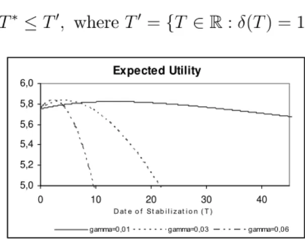
Figures 1 to 3 plot the expected utility and the median voter’s utility, as a function of the stabilization date, for di¤erent values of the growth rate of government expenditures ( ) and of inequality in income distribution ({med).27 Figure 4 plots the timing of reform as a function of inequality in
income distribution, while …gure 5 represents the date of stabilization as a
25Pevcin (2004) empirical results suggest that the optimal level of public expenditures
for European countries is approximately between 36 and 42 percent of GDP.
26This calibration was chosen in order to assure reasonable values for the parameters as
possible and to analyse how the delay lag responds to di¤erent initial situations. We do not intend to describe any particular economy with this example.
27For the discussion that follows, notice that {
med =ymed; as the GDP is normalized
function of the growth rate of government spending. In what follows, we take into account that the date of stabilization is constrained by the maximum tax rate possible, that is:
T T0
; where T0
=fT 2R: (T) = 1g
Expected Utility
5,0 5,2 5,4 5,6 5,8 6,0
0 10 20 30 40
D at e o f St ab i l i z at i o n ( T )
gamma=0,01 gamma=0,03 gamma=0,06
Figure 1: Expected utility for di¤erent values of the growth rate of Government expenditures ("gamma"):
Median voter's utility
3,2 3,4 3,6 3,8
0 10 20 30 40
D at e o f St ab i l i z at i o n ( T )
gamma=0,01 gamma=0,03 gamma=0,06
Figure 2: Median voter’s utility for di¤erent values of ("gamma"),
considering {med = 0:85:
Median voter's utility
-4 -2 0 2 4
0 5 10 15 20 25
D at e o f St ab i l i z at i o n ( T )
x_med=0,35 x_med=0,6 x_med=0,85
Figure 3: Median voter’s utility for di¤erent values of{med
("x_med"), considering = 0:03:
Figures 1 to 3 show that immediate stabilizations are not always the best choice, neither for the social planner, nor for the median voter, as the level of expenditures is initially too low. If = 0:03for instance, the optimal stabilization date would be in about4:5years, but, under majority voting, the stabilization date is 121percent higher, for a median income of85percent,28
what implies a government spending of 47 percent of GDP. If the median income decreases to 60percent of GDP, then the stabilization is undertaken after21:5years, implying a level of government spending about67percent of
GDP. If{med= 0:35;the restriction that imposes that the tax rate is less than
100percent binds, and hence the median voter would like to spend all income in public goods, imposing the maximum tax rate possible.29 This would imply
a level of government expenditures of 85 percent of GDP, attained after 29
years, and all income would be devoted to pay not only these expenditures, but also the interest over the level of debt. If we decrease the growth rate of government spending to1 percent, then both the optimal and the veri…ed dates of stabilization would triple, but nothing else changes, namely the attained level of expenditures, as long as the tax rate restriction is not biding, as in the case presented here. Hence, the delay lag also triples. A summary of results from this numerical example may be found in appendix B.
Date of Stabilization
0 10 20 30
0,3 0,4 0,5 0,6 0,7 0,8 0,9 1 R el at i v e med i an i nc o me
Optimal Verified
Figure 4: Date of stabilization and inequality in income distribution
for = 0:03:
Date of Stabilization
0 40 80 120 160 200
0,1% 1,1% 2,1% 3,1% 4,1% 5,1% Gr o w t h r at e o f Go v er nment s p end i ng
Optimal x_med=0,35 x_med=0,85
Figure 5: Date of stabilization and growth rate of Government
spending.
In …gure4, we can observe the behavior of the date of stabilization, de-pending on the median income, for = 0:03: For levels of median income below 47 percent of GDP, the tax rate is at its maximum, and no further delay is possible. Also, as one should expect, as inequality decreases, the veri…ed stabilization date approaches the optimal one. In an equalitarian so-ciety, there is no trend towards an excessive level of public expenditures. In …gure 5, we plot the date of stabilization as a function of the growth rate of government spending, for two di¤erent levels of inequality. For {med= 0:35;
the tax rate restriction is always biding, and hence the society uses all her in-come to provide public goods, and to pay for the interest of the accumulated de…cits. Notice that, even in this case, both the stabilization date under ma-jority voting and the delay lag are decreasing.30 If{
med= 0:85;then the tax 29On the contrary, Brazil and most Latin American countries have a median income
about 30-50 percent of GDP.
30The reason for this is the following. As the growth rate of government expenditures
rate restriction is only biding for values of lower than 0:002: The optimal stabilization date generates a tax rate lower than one for all values of the growth rate of government spending. Finally, observe that the gap between the optimal and the veri…ed stabilization dates shortens as increases.
Example 2 Consider now that the ‡ow utility has a constant relative risk
aversion (CRRA) speci…cation for g(t); i.e.:
ui(t) =ci(t) yi+
g(t)1 1
1 ; >0; 6= 1 (42)
This function allows for a di¤erent sensibility of the stabilization date to inequalities in income distribution. Depending on ; this may mitigate or accentuate some results found in the previous example.
The stabilization date
The optimal stabilization date is given by:
Topt;2 = 1ln
"
1=
g(0)
#
(43)
Where assumptionAimplies that 1= > g(0):The optimal level of
expen-ditures is theng(Topt;2) = 1= :Under majority voting, the date of stabilization can be written as:
Tmed;2 = 1ln
"
{ 1 med
1=
g(0)
#
(44)
Yielding a government spending of:
g(Tmed;2 ) = { 1
med
1=
={ 1= med g(T
;2
opt) (45)
Delay lag!
Computing the delay lag, we have:
Tmed;2 Topt;2 = 1lnh{ 1= med
i
(46)
Which is a straightforward generalization of the previous example. Ob-serve how in‡uences this lag, and consequently the gap between the level of expenditures chosen by majority voting and the optimal level:
d
d (T
;2
med T
;2
opt) =
1
2 ln{med <0 (47)
This implies that the higher the elasticity of marginal utility with re-spect to government expenditures, the lower the lag in the stabilization date under majority voting. Intuitively, a high implies that the marginal util-ity changes very quickly when these expenditures increase. Hence, although public goods are extremely important to economic agents, their bene…ts dis-sipate very quickly, and so it does not compensate for the median voter to delay stabilizations signi…catively. On the other hand, a lower originates a lesser response of the marginal utility to increases in expenditures, what may impel the median voter to choose signi…cative delays in order to appropriate these bene…ts. Notice that this idea can also be expressed in the following way:
d d
d
d{med T
;2
med T
;2
opt =
{ 1 med
2 <0 (48)
That is, the absolute value of a change in the delay lag motivated by a change in the median relative income depends negatively on :In other words, the higher the coe¢cient of relative risk aversion, the lower the responsiveness of the delay lag to a change in the median income.
Numerical results
We again set the same initial values for the parameters, except for :31
The optimal level of public expenditures is again set to 40 percent of GDP, which imply that must equal0:4 . This normalization is necessary so that we can analyze the delay lag using a benchmark case which remains invariant to changes is the economy. Concerning the elasticity of marginal utility, we consider only the case of >1here.32
This time, we do not analyze the response of the utility function to changes in the growth rate of government expenditures, because little is gained relatively to previous example, and hence we set at 3 percent. Instead, we inspect how di¤erent values of the coe¢cient of relative risk
31Once again, we do not intend to represent any economy, but to provide a ‡avor of the
reaction of the stabilization date to changes in the economic environment.
32Recall that when approaches one we originate the economy in the previous example.
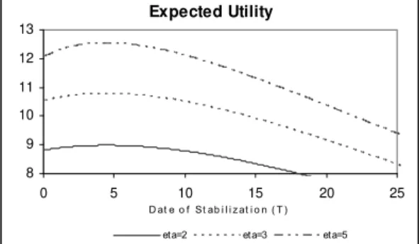
aversion may in‡uence the date of stabilization and the shape of the utility function. This is done precisely in …gures 6 to 8.33
Expected Utility
8 9 10 11 12 13
0 5 10 15 20 25
D at e o f St ab i l i z at i o n ( T ) et a=2 et a=3 et a=5
Figure 6: Expected utility for di¤erent values of ("eta"), calibrating such that = 0:4 :
Median voter's utility for x_med=0,35
-1 0 1 2 3 4
0 5 10 15 20 25
D at e o f St ab i l i z at i o n ( T ) et a=2 et a=3 et a=5
Figure 7: Median voter’s utility for di¤erent values of ("eta"),
considering {med = 0:35.
Median voter's utility for x_med=0,85
6 7 8 9 10 11
0 5 10 15 20 25
D at e o f St ab i l i z at i o n ( T ) et a=2 et a=3 et a=5
Figure 8: Median voter’s utility for di¤erent values of ("eta"),
considering {med= 0:85.
In these …gures, we can see that an increase in the coe¢cient of relative risk aversion does not change in fact the optimal date of stabilization, but it does in‡uence the date of stabilization chosen by the society. The higher is this coe¢cient, the sooner the median voter wants to stabilize, suggesting that the bene…ts from public spending dissipate faster, as observed before. Hence, even if the society is characterized by an extreme inequality, if = 5;
the delay lag is only 7 years, originating a government spending of49percent of GDP and a public debt of 41:7percent, what contrasts with the previous example, where the delay would be maximal. With a median income of 85
percent, the delay is negligible, as it originates a government expenditure
33Once again, in what follows, we take into account that the stabilization dates are
just slightly above the optimal one. A summary of these numerical results is presented in appendix C.
0
5
10 0.2 0.4
0.6 0.8
1 5
10 15 20 25 30 35 40 45
Relative Median Income ("xmed")
Date of Stabilization
Elasticity of Marginal Utility ("Eta") Years
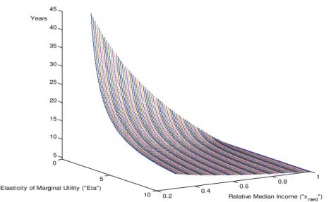
Figure 9: Date of stabilization as a function of the elasticity of marginal utility and the relative median income, for = 0:03: The lower plane
represents the optimal stabilization date.
Finally, …gure 9 shows precisely how the delay lag responds to changes in the elasticity of marginal utility and in the relative median income. We observe that the higher is this elasticity, the lower the delay and the respon-siveness of the delay lag to changes in the relative median income.
6
Concluding Remarks
median voter faces a lower cost of provision of public goods relatively to the society, while enjoying the same bene…ts. Hence, by delaying stabilizations and letting public expenditures grow above their optimal level, the median voter is able to expropriate the richest individuals of the society, indirectly transferring resources from these citizens to him.
We also illustrate that delays may be related to how the median voter is able to appropriate the bene…ts from additional expenditures in the society. If the bene…ts from these additional expenditures are not signi…cative, even high levels of inequality may not originate signi…cative delays. On the other hand, if the median voter is able to appropriate these bene…ts, for example, if public expenditures are devoted to redistribution policies, then delays in economic adjustments may be fairly signi…cative.
References
[1] Acemoglu, D. and Robinson, J. (2001), "A Theory of Political Tran-sitions," American Economic Review, vol. 91, No. 4, 938-963.
[2] Afonso, A. (2004), "Fiscal Sustainability: The Unpleasant European Case," mimeo, Cass Business School.
[3]Alesina, A. and Drazen, A. (1991), "Why are Stabilizations Delayed?,"
American Economic Review, vol. 81, No. 5, 1170-1188.
[4] Alesina, A. and Rodrik, D. (1994), "Distributive Politics and Eco-nomic Growth," Quarterly Journal of Economics, vol. 109, 465-490.
[5] Alesina, A. and Perotti, R. (1994), "The Political Economy of Budget De…cits," NBER Working Paper No. 4637.
[6]Cukierman, A. and Tommasi, M. (1998a), "When does it take a Nixon to go to China?", American Economic Review, 88, 180-97.
[7] ——— (1998b), "Credibility of Policymakers and of Economic Re-forms", in F. Sturzenegger and M. Tommasi, eds., The Political Economy of
Reform, Cambridge, MA: MIT Press.
[8] Downs, A. (1957), "An economic theory of democracy," New York:
Harper and Row.
[9]Drazen, A. (2001), "Political Economy in Macroeconomics",Princeton University Press, 2nd
edition.
[10]Drazen, A. and Grilli, V. (1993), "The Bene…t of Crises for Economic Reforms," American Economic Review, vol. 83, No. 3, 598-607.
[11]Fernandez R. and Rodrik, D. (1991), "Resistance to Reform: Status Quo Bias in the Presence of Individual Uncertainty", American Economic Review, vol. 81, 1146-55.
[12] Gouveia, M. and Masia, N. (1998), "Does the Median Voter Model Explain the Size of Government?: Evidence from the States," Public Choice, 97, 159-177.
[14] Husted, T. and Kenny, L. (1997), "The E¤ect of the Expansion of the Voting Franchise on the Size of Government," The Journal of Political Economy, vol. 105, No. 1, 54-82
[15] Krusell, P. and Rios-Rull, J. (1996), "Vested Interests in a Positive Theory of Stagnation and Growth", Review of Economic Studies, 63, 301-329.
[16] Lindert, P. (1996), "What Limits Social Spending,"Explorations in
Economic History, 33, 1-34.
[17] Martinelli, C. and Escorza, R. (2005), "When Are Stabilizations Delayed? - Alesina-Drazen Revised," Centro de Investigacion Economica, ITAM, Working Paper number 0408.
[18] Meltzer, A. and Richard, S. (1981), "A Rational Theory of the Size of Government," Journal of Political Economy, 89, 914-927.
[19] Meltzer, A. and Richard, S. (1983), "Tests of a Rational Theory of the Size of Government", Public Choice, 41, No. 3, 403-418.
[20] Milanovic, B. (2000), "The Median-voter Hypothesis, Income In-equality, and income redistribution: an empirical test with the required data," European Journal of Political Economy, vol. 16, 367-410.
[21]Olson, M., "The Rise and Decline of Nations",New Haven, CT: Yale University Press.
[22] Perotti, R. (1996), "Growth, Income Distribution and Democracy: What the Data Say," Journal of Economic Growth, vol. 1, No. 2, 149-187.
[23] Persson, T. and Tabellini, G. (1994), "Is Inequality Harmful for Growth?," American Economic Review, 84, 600-621.
[24] Pevcin, P. (2004), "Does Optimal Size of government Spending Ex-ist?," paper presented to the EGPA (European Group of Public Administra-tion) 2004 Annual Conference, Ljubljana, September.
[25] Roberts, K. (1977), "Voting over Income Tax Schedules,"Journal of
Public Economics, vol. 8, 329-340.
[26] Rodrik, D. (1993), "The Positive Economics of Policy Reform,"
[27] ——— (1996), "Understanding Economic Policy Reform," Journal
of Economic Literature, vol. 34, No. 1, 9-41.
[28] Romer, D. (2001), "Advanced Macroeconomics," McGraw-Hill, 2nd
edition.
[29] Romer, T. (1975), "Individual Welfare, Majority Voting, and the Properties of a Linear Income Tax," Journal of Public Economics, vol. 4, 163-185.
[30] Spolaore, Enrico (2004), "Adjustments in Di¤erent government Sys-tems," Economics and Politics, vol. 16, No.2, 117-146.
[31] Tornell, A. (1998), "Reform from Within," NBER Working Paper
#6497.
[32] Velasco, Andrés (1998), "A Model of Fiscal De…cits and Delayed Fiscal Reforms," in J. Poterba and J. Von Hagen, eds., Fiscal Institutions
7
Appendix
7.1
Appendix A: Proof of Proposition 1
First of all, recall that agent i maximizes:
Ui(T) = (49)
=
T
R
0
[ {i((1 ) (g(0) +rb(0)) + (g(t) +rb(t))) + v(g(t))]e rtdt+
+
1
R
T
[ {i[g(T) +rb(T)] + v(g(T))]e rtdt
Subject toT 0; and where:
g(t) =g(0) e t (50)
And:
b(t) =b(0) + (1 )g(0) [ (t; ; r; ) (t; = 0; r; )] (51)
With:
(t; ; r; ) = e
t er(1 )t
[ r(1 )] (52)
g(T) and b(T) are given by equations (50) (51) evaluated at t=T:
Using the Fundamental Theorem of Calculus and the Leibniz’s rule, and after a lot of extremely monotonous algebra that we do not replicate here, it can be shown that:
d
dT[Ui(T)] = rg(T)e
rT [ v0
(g(T)) {i] (53)
The First Order Condition yields:
rg(Ti )e
rTi [ v0
(g(Ti )) {i] 0 (54)
With strict equality if Ti >0: Hence,
Ti =
8 < :
1ln v0 1( 1{i)
g(0)
0
, if v0 1 1 {
i > g(0)
, if v0 1 1 {
To prove thatTi is the unique maximizer, it is enough to show that the utility function is strictly quasiconcave, that is: d
dT(E(U(T))) >0 ifT < Ti;
and dTd (E(U(T)))<0 if T > Ti : IfTi >0; we have:
d(Ui(T))
dT > 0,T <
1
ln 1
g(0) v
0 1( 1 {
i) =Ti (56)
d(Ui(T))
dT < 0,T >
1
ln 1
g(0) v
0 1( 1 {
i) =Ti (57)
ForTi = 0; we simply require that dTd (Ui(T))<0;8 T >0: This case is
trivial, so we skip it.
7.2
Appendix B: Numerical results presented in
exam-ple 1
1. The social planner outcome.
case 1 case 2 case 3
Growth rate of Gov. expenditures ( ) 0:01 0:03 0:06
Optimal date of stabilization (Topt;1) 13:4 4:5 2:2
Public debt (b(Topt;1)) - % GDP 17:8 5:6 2:7
Tax rate ( (Topt;1)) - % GDP 40:7 40:2 40:1
Optimal Gov. expenditures (g(Topt;1)) - % GDP 40:0 40:0 40:0
The social planner wants to implement the same level of public expen-ditures (40 percent), and hence, the higher the growth rate of government expenditures, the sooner the stabilization. Moreover, a lower implies a higher debt, because the interest is accumulated over more time.
2. The median voter’s outcome for a relative median income of0:85:
case 1 case 2 case 3
Growth rate of Gov. expenditures ( ) 0:01 0:03 0:06
Veri…ed date of stabilization (Tmed;1 ) 29:6 9:9 4:9
Delay lag (Tmed;1 Topt;1) 16:3 5:4 2:7
Public debt (b(Tmed;1 )) - % GDP 104 30:1 14:6
Tax rate ( (Tmed;1 )) - % GDP 51:2 48:3 47:6
For a median income of 85 percent of GDP, the attained level of public expenditures is always the same, regardless of the rate of growth of govern-ment spending. Hence, if is low, the economy takes more time of stabilize, in order to reach the desired level of public expenditures by the median voter, and if is high, this stabilization is attained sooner. Notice however that a low growth rate may imply a huge accumulation of debt, because the econ-omy is issuing debt to pay part of the interest that is accumulated before the stabilization takes place. Moreover, as one should expect, the delay lag is decreasing on the growth rate of government spending.
3. The median voter’s outcome for growth rate of government expendi-tures of 3 percent.
case 1 case 2 case 3
Median relative income ({med) 0:35 0:60 0:85
Veri…ed date of stabilization (Tmed;1 ) 29:5 21:5 9:9
Delay lag (Tmed;1 Topt;1) 25:0 17:0 5:4
Public debt (b(Tmed;1 )) - % GDP 379 174 30:2
Tax rate ( (Tmed;1 )) - % GDP 100:0 73:7 48:3
Veri…ed Gov. expenditures (g(Tmed;1 )) - % GDP 84:8 66:7 47:1
Here, in case 1 the restriction that imposes a tax rate no higher than100
percent binds, and hence the economy is forced to stabilize at T = 29:5:34;35
Obviously, the higher the median income, the lower the attained level of government expenditures and the lower the delay lag under majority voting. In fact, with no inequality in income distribution, the optimal and veri…ed dates of stabilization would coincide.
34Without this restriction, one would getTcb;1
med 39:5;but this would imply a tax rate
of147 percent, what is not feasible.
35Although not presented here, one can discover the median income above which the
restriction does not bind. Any median income above0:47will originate a stabilization date below29:5;and a tax rate below100percent. Hence, the stabilization date is constant for