UNIVERSIDADE TÉCNICA DE LISBOA F ACULDADE DEM OTRICIDADEH UMANA

(1)

UNIVERSIDADE TÉCNICA DE LISBOA

FACULDADE DE MOTRICIDADE HUMANA

Modeling intra- and inter-team spatial

interaction patterns in invasive team sports

Dissertação apresentada com vista à obtenção do grau de Doutor no Ramo de Motricidade Humana, Especialidade de Treino Desportivo, ao abrigo do artigo 33º do Decreto-Lei nº

107/2008, de 25 de Junho

Júri:

Presidente

Professora Doutora Maria Leonor Frazão Moniz Pereira da Silva Vogais

Doutor António Jaime da Eira Sampaio Doutor Pedro Simões Cristina de Freitas

Doutor Duarte Fernando Rosa Belo Patronilho Araújo Doutor Orlando de Jesus Semedo Mendes Fernandes Doutora Anna Georgievna Volossovitch

Sofia Cristina Carreiras Fonseca

(2)

(3)

iii

Team sports games are recognized as dynamic systems of interaction, where

individual and collective patterns of behavior emerge from a confluence of multiple

organismic, environmental and task-related constraints on the players. Researchers have

been interested in studying the dynamic interaction of these many degrees of freedom

for at least two decades considering various methods, approaches and techniques. In this

thesis we aimed to provide a fruitful contribution in this area of research presenting

innovative methods of analysis that overcome some identified methodological

limitations in measures that are often considered to (1) assess the complexity of

behavioral dynamic systems (ApEn) and (2) to describe the spatial interaction behavior

of a team.

Regarding the first issue, we have defined normalized measures of the original

ApEn to measure, and compare, the regularity of signals generated from any behavioral

system. These were tested and validated using two well-known data series of regular

(sine) and irregular (random) behavior. As for the second issue, we developed two new

models, Voronoi diagram (VD) and Superimposed Voronoi Diagram (SVD), from

which strong candidates to collective variables were derived: from the VD model we

defined the size of the dominant region (DR) and, from the SVD model, the percentage

of free area (%FA) and the maximum percentage of overlapped area (Max%OA). Given

that %FA that is largely dependent on the distance between each pair of exclusive

opponents, we have conjectured SVD patterns for two specific rules of dyadic

interaction: (1) exclusive pairing and (2) random interaction. While the former rule was

thought to be associated with a specific defensive method, the man-to-man defense, the

second rule is associated with a reference spatial pattern used for analysis purposes.

(4)

iv

generate reference values of %FA. As for the Max%OA, data from simulated SVD

patters have shown that this variable is inversely associated with the number of

opponent neighbors, i.e., the more the opponents the smaller the Max%OA.

Results from formal applications of the described methods have suggested the

following: (1) having considered data signals from the collective variable that describes

the dyadic sub-system in rugby union, we found that the physical contact between the

players (tackle) increases the complexity of the emergent behavior, making this more

predictable in try situations; (2) in Futsal (5 vs 4+GK in a limited play area of

20×20m2), the size of the DR was measured to assess how teams manage space – the

attacking team has presented greater DR than the defending team throughout the task,

also, the attackers presented a more regular spatial behavior, which means spatial

behavior of the team defending is more unpredictable; (3) the %FA has captured the

presence of low levels of exclusive dyadic interaction when the defense team has

numerical disadvantage; (4) the Max%OA was able to identify the attacker under more

pressure.

(5)

v

Jogos desportivos colectivos podem ser considerados como sistemas dinâmicos de interação, onde padrões de comportamento individual e coletivo emergem de uma confluência de vários constrangimentos (indivíduo, ambiente e tarefa) na acção dos joagadores. Há pelo menos 20 anos, os investigadores têm-se interessado pelo estudo da interação dinâmica desta multiplicidade de graus de liberdade, considerando para tal vários métodos de análise, abordagens e técnicas. Pretende-se que o trabalho

apresentado nesta tese constitua uma contribuição frutífera para esta área de

investigação, sendo aqui apresentados métodos inovadores de análise que pretendem superar algumas limitações metodológicas identificadas nas medidas que são muitas vezes consideradas (1) para avaliar a complexidade de sistemas dinâmicos (ApEn) e (2) para descrever o comportamento de interação espacial entre equipas.

Quanto à primeira questão, foram aqui propostas medidas normalizadas de entropia aproximada (ApEn) para medir e comparar a regularidade de sinais gerados por qualquer sistema comportamental. Estas medidas foram testadas e validadas

considerando séries de referência para comportamento regular (função seno) e irregular (função geradora de números aleatório). Quanto à segunda questão, foram considerados dois novos modelos de análise, os diagramas de Voronoi (DV) e os Diagramas de Voronoi Sobrepostos (DVS), dos quais foram derivadas medidas candidatas a variáveis coletivas: a partir do modelo DV definimos a área da região dominante (RD) e, a partir do modelo DVS, a percentagem de área livre (AL%) e máxima percentagem de área sobreposta (Max%AS). Dado que a AL% dependente da distância interpessoal de diades exclusivas, conjecturamos padrões DVS de acordo com duas regras de interacção

diádica: (1) emparelhamento exclusivo e (2) interacção aleatória. A primeira regra está teoricamente associada ao método de defesa homem-a-homem e a segunda regra está associado a um padrão de referência espacial utilizado para análise. Foram simulados padrões de distribuição espacial sob estas duas regras, e de acordo com as características da tarefa em estudo (5 vs 4 + GR numa área de 20×20m2), para gerar valores de

(6)

vi

verificou-se que o contacto físico entre os jogadores (placagem) aumenta a

complexidade do comportamento emergente, tornando-o mais previsível em situações em que o Ensaio é marcado, (2) no Futsal (5 vs 4 + GK numa área de 20×20m2), o tamanho da RD foi medida para avaliar como as equipas gerem o espaço – a equipa que ataca apresenta uma RD maior do que a equipa que defende, e os atacantes apresentam um comportamento espacial mais regular, o que significa que o comportamento espacial da equipa que defende é mais imprevisível; (3) a %AL permitiu detectar baixos níveis de interação diádica exclusiva quando a equipa que está a defender se encontra em desvantagem numérica; e (4) a Max%AS permite identificar o atacante que se encontra sob mais pressão.

(7)

7

List of Figures

Figure 1: Three players of a team at the same interpersonal distances but placed in different locations form the same geometric shape as it does not account for the boundaries of the field (the black dots are the 2D spatial representation of the players). ... 14

Figure 2: Three players of a team at the same interpersonal distances but placed in different locations form a very different spatial pattern as assessed by a Voronoi diagram, which partitions the field taking into account its boundaries (the black dots are the 2D spatial representation of the players). ... 15

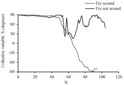
Figure 3: Example data for the collective variable X measured in a successful trial (Try scored) and in a unsuccessful trial (Try not scored) ... 28

Figure 4: (a) Normalized entropy measures and (b) original entropy measure

calculated for sine and random series data of different lengths (N) ... 29

Figure 5: Mean approximate entropy for each of the two task outcomes using

ApenRatioRandom and ApEnRatioShuffle ... 30

Figure 6: 95th percentile envelopes of ApEnRatioRandom for random series of different lengths (N) and the fitted logarithm curves for the upper and lower bounds ... 31

Figure 7: Example of spatial distribution patterns (a) random, (b) regular and (c) clustered. ... 38

Figure 8: Example of a Voronoi diagram generated for the set of points represented in the figure. ... 39

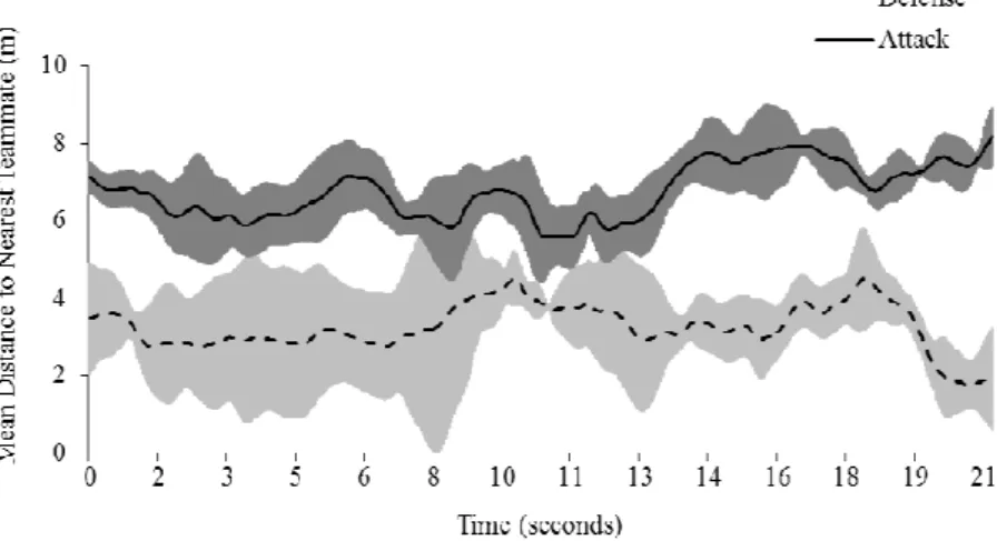
Figure 9: Mean distance to nearest teammate distance, across time, for the attacker and defender teams in a randomly selected play (error bars represent the standard deviation). ... 43

Figure 10: Mean area of the dominant region, across time, for the attacker and

(10)

10

Figure 11: Comparison of the mean entropy of the distance to nearest teammate (DistNT) and area of the dominant region (AreaDR) between teams in the same play. Error bars represent the standard deviation (*** p<0.001). ... 45

Figure 12: Variables for describing team spatial organization of two opponent teams (players of each team are represented by black dots and triangles, respectively, grey players on the top and bottom of the field are the goalkeepers) – (a) convex hull, (b) horizontal and vertical stretch and (c) centroid position (red dots). ... 55

Figure 13: The same spatial configuration of two teams 5+ GK vs 5+GK (players of each team are represented by black dots and triangles, respectively, grey players on the top and bottom of the field are the goalkeepers) measured using the area of the respective convex hull (shaded areas) in three very different scenarios (a, b and c). ... 55

Figure 14: Example of a set of points in a plane (a) and respective Voronoi diagram (b). ... 56

Figure 15: Construction of the superimposed Voronoi diagram (at bottom) from considering, separately the Voronoi diagrams for team A (black dots) and team B (white dots)... 57

Figure 16: Measures from the superimposed Voronoi diagram (SVD): (a) shaded grey areas are the maximum Overlapped Area for each player of the team represented with black dots; (b) the sum of the shaded black area is the Free Area. ... 58

Figure 17: Example of a generated SV in a situation where (a) players from both teams (grey and black dots) are randomly distributed in the field and (b) defender players, grey dots, are exclusively paired with the attacker players, black dots, that are closer to the goal. The GK (red dot) is in both cases fixed at position (10, 18). The arrow indicates the direction of the attack... 59

(11)

11

Figure 19: Mean of the maximum percentage of Overlapped Area (Max%OA) calculated for a player in situations where the number of players inside his Voronoi area varies from 1 to 5. The error bars represent the standard deviation. ... 61

Figure 20: Observed %FA (percentage of Free Area) in a sample of 4 trials (solid black line) and the 95% confidence interval for absence of interaction (dashed grey lines). Values within the dashed lines (0.22, 0.50) indicate low levels of exclusive dyadic

interaction. ... 62

(12)

12

Chapter 1: General introduction

Framework

Team sports of an invasive nature are those sports where each of the two competing

teams tries, simultaneously, to gain possession of an object, e.g. the ball, in order to move it

across a field toward the goal of the other team, and to prevent the opposing team from doing

the same thing (Bayer, 1994). Thus, during a game, the two teams act concurrently and their

behavior alternates between attempting to score, if they are in possession of the ball, and

preventing the other team to score, if they are not in possession of the ball.

During a game, players from both teams act continuously according to game rules and

principles, but fundamentally according to their perception of, and interaction with, the

information available in the environment (Araújo, Davids & Hristovskic, 2006). According to

the same author, behavior in team sports ecologically emerges from a confluence of multiple

organismic (e.g. fatigue), environmental (e.g. size of the field) and task-related (e.g. defend)

constraints on the players (Newell, 1986; Handford, Bennet & Button, 1997). Given these

many degrees of freedom, behavior in team sports can then be seen as a dynamic system

(Gréhaigne, Bouthier & David, 1997; McGarry et al., 2002).

In general, dynamical systems have nonlinear properties, and therefore they cannot be

studied using linear methods of analysis. Hence, dynamical system has been approached by

means of synergetic and nonlinear equations (Haken, 1987; Davids et al., 2003), which are

defined based on order and control parameters, the ‘yin and yang’ of the synergetic approach

(Kelso, 1995). An order parameter, or collective variable, is a low-dimensional variable that

capture the dynamic behavior of the system, and a control parameter are properties that

(13)

13

parameter, the order parameter can change from one state to another, with fluctuations during

transition between states (Kelso, 1995; Stergiou, 2004). Thus, the choice of a collective

variable is a critical step for characterizing a dynamic system, and depending on the level of

analysis to be undertaken, this could be quite difficult to accomplish (Thelen & Smith, 2006).

Studying behavior in sports games by mean of collective variables was first

considered in a dyadic level of interaction, specifically, in individual sports, such as squash

(McGarry & Franks, 1996; McGarry, Khan & Franks, 1999; McGarry, 2005) and tennis

(Palut & Zanone, 2005; Lames, 2006) and in dyads from team sports, such basketball (Araújo

et al., 2004; Cordovil et al., 2009) and rugby (Passos et al., 2006; Passos et al., 2008). The

collective variables suggested to describe the behavioral dyadic system were mainly distance

related measures, as suggested by Schmidt, O’Brien & Sysko (1999). Results from these

innovative studies have contributed greatly for a better understanding of the dynamical

interaction behavior in sports. Nevertheless, a comprehension of interaction behavior at a

higher level, i.e., team level, could not be inferred from the former, neither those collective

variables could be effectively applied in systems with multi-players (McGarry, 2009).

Following this, some ideas were developed regarding holistic measures that could be

considered for describing team behavior, at a collective level, as a dynamical system

(Schöllhorn, 2003). It is commonly accepted among researchers and coaches that teams’

positioning and distribution in the field is often associated to strategic decisions, principles

and prescriptions (Garganta, 2009), which are likely to be printed in the behavioral patterns

observed during a game. Hence, some quantitative measures extracted from the positioning of

all teammates have, in theory, potential to be considered collective variables. The covered

(14)

14

putted forward by Schöllhorn (2003) and somehow adapted in posterior studies, as those

described next.

Some of the variables currently considered as capable of capturing the dynamics of

team behavior during a game are the convex hull (Frencken et al., 2011), the stretch index

(Bourbousson, Sève, & McGarry, 2010a) and simple measurements derived from the average

position (centroid) of the whole team (Frencken & Lemmink, 2008; Bourbousson, Sève, &

McGarry, 2010b; Frencken et al., 2011; Sampaio & Maças, 2012). Despite the ability of these

variables of describing some characteristics of the underlying dynamical system, they are

calculated neglecting one of the major characteristics of the structural dimension, this being

the boundaries which establish the frontiers of the system (McGarry, 2009). This is illustrated

using a simple example in Figure 1.

Figure 1: Three players of a team at the same interpersonal distances but placed in different locations form the same geometric shape as it does not account for the boundaries of the field (the black dots are the 2D spatial representation of the players).

Another drawback is that those measures are often calculated for each team

separately, not considering information regarding the distribution characteristics of the other.

This limits the analysis of intra- and inter- team interaction behaviors as, conceptually,

interaction between and among groups assumes a global interaction, where all players play a

(15)

15

There are, however, spatial construction, named Voronoi diagram (Dirichlet, 1850,

Voronoi, 1908), that partition the area of interest, the field, into as many cells as the existing

points, players, taking into account the position of all players and the limits of the field.

These diagrams have already been successfully applied in a variety of game settings, namely,

real soccer games (Taki, Hasegawa & Fukumura, 1996), electronic soccer games (Kim,

2004), robotic soccer (Law, 2005) and real hockey games (Fujimura & Sugihara, 2005), in

which the authors suggested some variables to characterize players individual and collective

behavior. However, this was not approached under the theory of the dynamical systems.

As this particular partition of space captures some essential details of players’

distribution, which are neglected in other more popular methods (Figure 2 in opposition to

Figure 1), it is possible to recognize the potential of the Voronoi diagrams for studying the

spatial characteristics of the team behavior and for deriving from these diagrams some strong

candidates to collective variables.

Figure 2: Three players of a team at the same interpersonal distances but placed in different locations form a very different spatial pattern as assessed by a Voronoi diagram, which partitions the field taking into account its boundaries (the black dots are the 2D spatial representation of the players).

When the collective variable(s) of a dynamical system is defined, it is possible to

capture its behavior by measuring that variable across time. The characteristics of the

observed dynamical system, such as self-organization, perturbations, critical fluctuations,

(16)

16

can also be assessed by studying the characteristics of the generated data series. The

regularity of a signal relates to the complexity of the system generating it (Pincus, 1995),

thus, by quantifying regularity it is possible to measure complexity.

The Approximate Entropy (ApEn) is a nonlinear measure of regularity in behaviors of

complex systems (Pincus, 1991) and it was much applied in the analysis of physiological

time series such as heart rate variability, electrocardiogram measures, respiration, anesthesia,

gene sequences, pulse waveform and electroencephalography (Xu, Wang & Wang, 2005).

Such systems can be observed in a fixed time window, often rather long, so that each of their

realizations produces a signal of a pre-determined fixed length, which is a requirement for

applying the ApEn measure. Unlike these, team sports’ dynamical systems cannot be framed

temporally as they evolve across time towards a certain goal and finish whenever that goal is

achieved by one of the two parties involved, being possible to vary between very short and

very long series. Clearly, this is a limitation that needed to be addressed as dynamical system

has become a dominant approach to the analysis of team sports’ behavior in different levels

and dimensions.

Some authors have already suggested modified measures of the original ApEn, such

as the sample entropy (Richman, & Moorman, 2000), which are less dependent on record

length and more stable for short series, however, these do not allow, for example, revisiting

studies where the old ApEn was applied and compare their complexity with the complexity of

(17)

17

Aims

In aim of the present research work was, firstly, to address the identified limitations

on applying the ApEn measure to quantify the regularity of time series data from collective

variables measured in team sports dynamical systems. Secondly, to develop models for

formally describing behavioral patterns of spatial interaction in team sports using Voronoi

diagrams. From these models, we aimed to derive reliable collective variables for assessing

inter- and intra-team interaction behavior at different levels, and to establish reference values

for specific patterns of interaction in order to distinguish modes of spatial interaction

behavior during a game.

Outline

The thesis is constituted by four chapters, the first two (Chapter 2 and Chapter 3) are

articles that were submitted, revised and accepted for publication in the course of this

process.

Chapter 2 presents normalized measures of approximate entropy (ApEn) which allow

quantifying the complexity of a system responsible for a given time series signal. This work

emerged from an identified limitation on using the original ApEn measure in team sports’

data given that, in the majority of situations, the signals under study are of varying lengths

and are likely to be small (less than 50 data points). Thus, in order to measure and compare

the regularity of team and players’ behavior across a game, plays or trials, we suggest these

normalized measures. In this study we have consider an application of the new ApEn

measures in rugby union attacker-defender system.

Chapter 3 describes the results from an application of Voronoi diagrams (VD) to

(18)

18

the spatial distribution of players in the field relates with the spatial interaction behavior

established at player and team levels, and hence, this will vary according to the modes of

interaction assumed. We suggest collective spatial variables, derived from the mentioned

spatial tessellation, for describing intra-team interaction behavior in invasive team sports.

Chapter 4 presents a paper recently submitted for publication to the journal of

Behavior Research Methods and it is, to date, waiting a revision. Here is presented a novel

conceptual spatial model for assessing spatial configuration patterns in invasive team sports

based on the previously introduced VD. This Superimposed Voronoi diagram (SVD) model,

as it was named, was applied to Futsal data and the collective variables suggested for

measuring spatial interaction at team and player levels were then tested. Additionally, for this

particular data, reference values for two modes of spatial interaction modes were calculated

using data from simulated spatial patterns and used for identifying patterns of spatial

behavior in Futsal.

Finally, in Chapter 5, a general discussion of the main results from the three articles is

presented, along with some final considerations about the contribution of this work to both

(19)

19

References

Araújo, D., Davids, K., & Hristovskic, R. (2006). The ecological dynamics of decision making in sport. Psychology of Sport and Exercise, 7, 653–676.

Araújo, D., Davids, K., Bennett, S. J., Button, C., & Chapman, G. (2004). Emergence of sport skills under constraints. In A. M. Williams, & N. J. Hodges (Eds.), Skill Acquisition

in Sport: Research, Theory and Practice (pp. 409-433). London: Routledge, Taylor & Francis.

Bayer, C. (1994). O ensino dos desportos coletivos. Lisboa, Dinalivro.

Bourbousson, J., Sève, C., & McGarry, T. (2010a). Space-time coordination dynamics in basketball: Part 1. Intra- and inter-couplings among player dyads. Journal of Sports

Sciences, 28(3), 1-9.

Bourbousson, J., Sève, C., & McGarry, T. (2010b). Space-time coordination dynamics in basketball: Part 2. The interaction between the two teams. Journal of Sports Sciences,

28(3), 349-358.

Cordovil, R., Araújo, D., Davids, K., Gouveia, L., Barreiros, J., Fernandes, O., et al. (2009). The influence of instructions and body-scaling as constraints on decision-making processes in team sports. European Journal of Sport Science, 9(3), 169 – 179.

Davids, K., Glazier, P., Duarte, A., & Bartlett, R. (2003). Movement Systems as Dynamical Systems: The Functional Role of Variability and its Implications for Sports Medicine. Sports Medicine, 33(4), 245-260

Dirichlet, G.L. (1850). Über die Reduktion der positiven quadratischen Formen mit drei unbestimmten ganzen Zahlen. Journal für die Reine und Angewandte Mathematik,40, 209-227.

Frencken W., Lemmink, K., Delleman, N., & Visscher, C. (2011). Oscillations of centroid position and surface area of soccer teams in small sided games. European Journal of

(20)

20

Frencken, W., & Lemmink, K. (2008). Team kinematics of small-sided soccer games. A systematic approach. In T. Reilly and F. Korkusuz (Eds.), Science and football VI:

Proceedings of the 6th World (pp. 161-166). New York, NY: Routledge.

Garganta, J. (2009). Trends of tactical performance analysis in team sports: bridging the gap between research, training and competition. Revista Portuguesa de Ciências do

Desporto, 9(1), 81-89.

Gréhaine, J, Bouthier, D., & David, B. (1997). Dynamic-system analysis of opponent relationships in collective actions in soccer. Journal of Sports Sciences, 15(2), 137-149.

Haken, H. (1987). Information Compression in Biological Systems. Biological

Cybernetics, 56, 11-17.

Handford, C., Davids, K., Bennett, S., & Button, C. (1997). Skill acquisition in sport: Some applications of an evolving practice ecology. Journal of Sports Science, 15(6), 621-640.

Kelso, J.A.S. (1995). Dynamic Patterns: The Self-Organization of Brain and Behavior. Cambridge, Massachusetts: MIT Press.

Kim, S. (2004). Voronoi Analysis of a Soccer Game. Nonlinear Analysis: Modelling

and Control, 9(3), 233-240.

Lames, M. (2006). Modelling the interaction in game sports- Relative phase and moving correlations. Journal of Sports Science and Medicine, 5, 556-560.

Law, J. (2005). Analysis of Multi-Robot Cooperation using Voronoi Diagrams. Proceedings of the 3rd International Kemurdjian Workshop “Planetary rovers, space robotics and Earth-based robots-2005”, St Petersburg, Russia, October 2005

McGarry T. (2009). Applied and theoretical perspectives of performance analysis in sport: Scientific issues and challenges. International Journal of Performance Analysis in

(21)

21

McGarry, T. (2005). Soccer as a dynamical system: Some theoretical considerations. In T. Reilly, J. Cabri, & D. Araújo (Eds.), Science and Football V, (pp. 551-560). London: Routledge.

McGarry, T., Anderson, D.I., Wallace, S.A., Hughes, M.D., & Franks, I.M. (2002). Sport competition as a dynamical self-organizing system. Journal of Sports Sciences, 20:10, 771-781.

McGarry, T., Khan, M. A., & Franks, I. M. (1999). On the presence and absence of behavioural traits in sport: An example from championship squash match-play. Journal of

Sports Sciences, 17, 297-311.

McGarry, T., & Franks, I. M. (1996). Development, application, and limitation of a stochastic Markov model in explaining championship squash performance. Research

Quarterly for Exercise and Sport, 67, 406-415.

Palut, Y., & Zanone, P. G. (2005). A dynamical analysis of tennis: Concepts and data.

Journal of Sports Sciences, 23, 1021-1032.

Passos, P., Araújo, D., Davids, K., Gouveia, L., Milho, J., & Serpa, S. (2008). Information-governing dynamics of attacker- defender interactions in youth rugby union.

Journal of Sports Sciences, 26, 1421-1429.

Passos, P., Araújo, D., Davids, K., Gouveia, L., & Serpa, S. (2006). Interpersonal dynamics in sports: The role of artificial networks and 3-D analysis, Behavior Research

Methods, 38(4) 683-691.

Pincus, S. (1995). Approximate entropy (ApEn) as a complexity measure. Chaos, 5, 110-117.

Pincus, S. (1991). Approximate entropy as a measure of system complexity.

Proceedings of the National Academy of Sciences, 88, 2297-2301.

(22)

22

Sampaio, J. & Maçãs, V. (2012). Measuring tactical behaviour in football.

International Journal of Sports Medicine, 33(5), 395-401.

Schöllhorn, W. (2003). Coordination dynamics and its consequences on sports.

International Journal of Computer Science in Sport, 2, 40-46.

Schmidt, R. C., O’Brien, B., & Sysko, R. (1999). Self- organization of between-persons cooperative tasks and possible applications to sport. International Journal of Sport

Psychology, 30, 558-579.

Stergiou, N (2004) Innovative Analysis of Human Movement. Human Kinetics, Champaign, IL.

Taki, T., Hasegawa, J. & Fukumura, T. (1996). Development of Motion Analysis System for Quantitative Evaluation of Teamwork in Soccer Games, IEEE, 815-118.

Thelen, E. & Smith, L.B. (2006). Dynamic Systems Theories. In Handbook of Child Psychology, Volume 1, Theoretical Models of Human Development, 6th Edition, William Damon (Editor), Richard M. Lerner (Volume editor), pp. 258-312.

Voronoi, G. (1908). Nouvelles applications des paramètres continus à la théorie des formes quadratiques. Journal für die Reine und Angewandte Mathematik,134, 198-287.

Xu, L.S., Wang, K.Q., & Wang, L. (2005). Gaussian kernel approximate entropy algorithm for analyzing irregularity of time series. Proceedings of the 4th International

(23)

23

Chapter 2: Approximate entropy normalized measures for

analyzing social neurobiological systems

Sofia Fonseca, João Milho, Pedro Passos, Duarte Araújo & Keith Davids

DOI:10.1080/00222895.2012.668233

Abstract

When considering time series data of variables describing agent interactions in social

neurobiological systems, measures of regularity can provide a global understanding of such

system behaviors. Approximate entropy (ApEn) was introduced as a nonlinear measure to

assess the complexity of a system behavior by quantifying the regularity of the generated

time series. However, ApEn is not reliable when assessing and comparing the regularity of

data series with short or inconsistent lengths, which often occur in studies of social

neurobiological systems, particularly in dyadic human movement systems. Here, we present

two normalized, non-modified, measures of regularity derived from the original ApEn which

are less dependent on time series length. The validity of the suggested measures is tested in

well-established series (random and sine) prior to their empirical application, describing the

dyadic behavior of athletes in team games. We consider one of the ApEn normalized

measures to generate the 95th percentile envelopes that can be used to test whether a

particular social neurobiological system is highly complex, i.e., generates highly

unpredictable time series. Results demonstrated that suggested measures may be considered

as valid instruments for measuring and comparing complexity in systems that produce time

series with inconsistent lengths.

(24)

24

Introduction

Approximate Entropy (ApEn) was first introduced in 1991 by Pincus as a nonlinear

measure to quantify regularity in the behaviors of complex systems (Pincus, 1991). The

regularity of a signal relates to the complexity of the system generating it (Pincus, 1995),

thus, the greater the value of ApEn, the lower the regularity of the time series, and the greater

the complexity of the system under study. ApEn values vary between 0 and 2, with high

values identifying data series with less regular and predictable patterns, and low values

associated with data series containing many repetitive patterns, i.e., data which are more

regular and more predictable. Since its introduction, ApEn has been established as a measure

of regularity in a time series, with numerous applications in analysis of physiological time

series such as heart rate variability, electrocardiogram measures, respiration, anesthesia, gene

sequences, pulse waveform and electroencephalography (Xu, Wang & Wang, 2005).

A major interest when analyzing the complexity of physiological systems is to

compare the regularity of a given time series between different groups, for instance, compare

the ApEn of pulse data records in healthy persons, inpatients with cardiovascular disease and

inpatients without any cardiovascular disorder (Wang, Xu, Li, Zhang, Li & Wang, 2003).

However, given that ApEn values are highly dependent on times series length, and are

particularly unstable for short time series (e.g. Pincus & Golberger, 1994; Xu et al., 2005;

Richman, 2007), the application of such a regularity measure is only recommended when

considering signals of the same length, preferably with at least 50 data points (Stergiou,

Buzzi, Kurz, & Heidel, 2004). To ensure such conditions, when considering physiological

(25)

25

of time and data are collected at the same rate (Pincus, & Viscarello, 1992; Ryan,

Goldberger, Pincus, Mietus, & Lipsitz, 1994; Pincus, Padmanabhan, Lemon, Randolph, &

Midgley, 1998; Wang et. al, 2003).

When the conditions above cannot be guaranteed, modified measures of the original

ApEn can be applied, e.g. sample entropy (Richman, & Moorman, 2000), Gaussian Kernel

approximate entropy (Xu et al., 2005), modified sample entropy (Xie, He, & Lui, 2008) and

Fuzzy approximate entropy (Chen, Zhuang, Yu, & Wang, 2008). These measures have been

shown to be less dependent on record length and more stable for short series.

In the study of social neurobiological systems, such as flocking birds, schooling fish,

herding animals, human societies and sports teams (Couzin, 2007; Sumpter, 2006), unlike

physiological systems, it may not be possible to ensure that all system output samples are of

the same length. This is particularly difficult in studying social neurobiological systems

because of the continuous interactions of system agents in tasks where a specific performance

goal has to be achieved. Since the length of the captured time series is dependent on the time

required by the agents to conclude a particular performance task (as exemplified by an

attacking or defending performance sub-phase in a team game), the use of ApEn for assessing

regularity is not advisable. Modified measures of regularity, such as those mentioned above,

could be applied here however, we suggest in this paper two normalized measures of the

original ApEn. By applying these new measures one can compute a straightforward

normalization of any ApEn value where the original ApEn was used, which allows a reliable

(26)

26

Material and Methods

Given a data series with N points, say {x1, x2, …, xN}, ApEn (m, r, N) can be used to measure

the logarithmic likelihood that runs of patterns with m points that are close, remain close

within a tolerance factor r in ensuing incremental comparisons (Pincus, 1991), i.e., to

measure the predictability of the data series. In order to compute ApEn (m, r, N), the

parameters m, the length of compared runs, and r, the tolerance factor, need to be fixed for all

calculations to ensure reliable analysis (Pincus, & Goldberger, 1994). In our analysis, as

suggested in studies of other neurobiological systems, we considered m = 2 and r = 0.2. All

calculations were performed in Matlab (7.6.0) using routines written for this purpose

(Kaplan, & Saffin, 2009).

The techniques for normalization considered here are based on the ratio between an

observed ApEn value and a threshold reference ApEn value, for a specific data series length.

This normalization allows the regularity of data series of different lengths to be compared.

Our first normalized measure, designated ApEnRatioRandom, is given by

100 ) , 2 . 0 , 2 ( ApEn ) , 2 . 0 , 2 ( ApEn ApEn ₁₀₀ 1 m RatioRando

∑

₌ = i U X i N N

Here, the regularity of the data series X={x1, x2, …, xN} is quantified by means of the

ratio between its original ApEn value, ApEn (2, 0.2, N)X , and the mean ApEn calculated in

100 random series Ui with the same length N. Note that for each generated random series, Ui,

the corresponding approximate entropy,

i U N) , 2 . 0 , 2 (

ApEn , represents a maximum value of

approximate entropy for that particular length. Hence, ApEn (2, 0.2, N)X is normalized with

(27)

27

Our second normalized measure, designated ApEnRatioShuffle, is given by

100 ) , 2 . 0 , 2 ( ApEn ) , 2 . 0 , 2 ( ApEn ApEn ₁₀₀ 1 le RatioShuff

∑

₌ = i S X i N N

Here, the regularity of the data series X={x1, x2, …, xN} is given by the ratio

between its original ApEn value, ApEn (2, 0.2, N)X , and the mean ApEn calculated in 100

shuffled replicas Si of the original data. Note that for each shuffled replica of X, Si, the

corresponding approximate entropy,

i S N) , 2 . 0 , 2 (

ApEn , represents a maximum value of

approximate entropy for that particular set of points. Hence, ApEn (2, 0.2, N)X is normalized

with respect to a maximum value of ApEn of that particular set of points. In both methods

described here, low values of the corresponding measures will indicate that the time series

under study is generated by a social neurobiological system that is less predictable than

random time series of the same length.

For testing the methods presented in this paper, we considered data from a dyadic

human movement system; more precisely, a rugby union attacker-defender system where the

attacker aims to score and the defender tries to prevent it. Results should be in accordance

with findings in the literature that suggest that physical contact between an attacker and

defender increases the complexity of this system (Passos et al., 2009), making the dyadic

sub-system behaviors that emerge in try situations (success for the attacker) more predictable than

in tackle situations (success for the defender) where players do experience physical contact.

In this regard, the interactive behaviors that emerges in each trial of this social

neurobiological system is accurately measured, across its duration, by a one-dimensional

variable X defined in previous work by Passos et al. (2009) and designated as collective

(28)

28

formally given by the value of the angle between the defender–attacker vector and a

horizontal line parallel to the try line with the origin in the defender. The values of X range

from -90º to 90º, which occur when an attacker and defender are in the same vertical position,

being 90º when the defender is closer to the try line and -90º when the attacker is closer to the

try line. X is zero when attacker and defender are in the same horizontal position.

To assess the regularity of this collective variable, we considered 47 experimental

dyadic trials in which participants were male rugby players aged 11–12 years, with an

average of 4.0 ± 0.5 years of rugby practice. Treatment of participants was in accordance

with the ethical standards of American Psychological Association (APA). Trials were

performed on a field of 5 m width × 10 m depth and two fixed digital video cameras at 25 Hz

were used to capture players’ movements. The angle given by the variable X was calculated

from players’ trajectory motion data extracted from the videos using the methodology

described in detail in Passos et al. (2009). Figure 3 displays two examples of these data, one

from a successful situation (try scored) and the other from an unsuccessful situation (try not

scored).

(29)

29

The 47 data series analyzed, try scored (n=20) and try not scored (n=27), had a record

length ranging from 69 to 230 data points (112 ± 36.3). Both normalized measures of ApEn

were calculated and comparative statistical analyses were performed using non-parametric

tests (Mann-Whitney test) due to lack of normality in the data and the small sample size. The

level of statistical significance was fixed at 5%.

Results

The normalized measures of ApEn suggested in this paper, ApEnRatioRandom and

ApEnRatioShuffle were tested in regard to the series length effect. An application of these two

well-known data series (sine and random) with different lengths, has shown the advantages of

these (Figure 4a) in comparison to the original ApEn measure (Figure 4b).

(a) (b)

Figure 4: (a) Normalized entropy measures and (b) original entropy measure calculated for sine and

random series data of different lengths (N)

Both normalized measures appeared to be less dependent on record length for both

data series, reaching stability for small lengths. This observation reinforces the need of

considering more reliable measures for analyzing complexity in systems that produce time

series with inconsistent lengths, a typical occurrence when studying social neurobiological

(30)

30

approximate entropy comparisons (Stergiou et al., 2004). In a specific application of these

measures to a dyadic sub-system (1v1) interaction in the team sport of rugby union, where

physical contact is associated with less regular interaction behaviors, both ApEn normalized

measures indicated, accordingly, greater unpredictability in situations with effective contact

between the players, i.e. an attacker was tackled by an opposing defender (try not scored) (see

Figure 5).

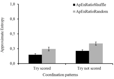
Figure 5: Mean approximate entropy for each of the two task outcomes using ApenRatioRandom and ApEnRatioShuffle

Using the non-parametric Mann-Whitney test, significant differences were found

between the two task outcomes for ApEnRatioRandom(p=0.0196) and ApEnRatioShuffle (p=0.0185),

confirming that behavioral outcomes in try situations are more regular than tackle situations.

Given the similarity of both measures, we considered the ApEnRatioRandom to determine

the 95th percentile envelope of this normalized measure, calculated from 100 simulations of

(31)

31

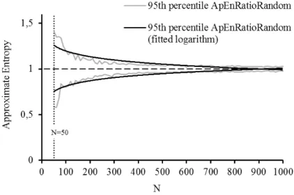
Figure 6: 95th percentile envelopes of ApEnRatioRandom for random series of different lengths (N) and the fitted logarithm curves for the upper and lower bounds

The logarithm curves fitted to the upper (U) and lower (L) bounds of the 95th

percentile of the ApenRatioRandom for random time series with length greater than 50 are given

by

( )

95 RatioRandom

ApEn th 0.09ln 1.6089

U = − N +

( )

95 RatioRandom

ApEn th 0.0845ln 0.4233

L = N +

with a corresponding R2 for the logarithm fitting of 0.752 and 0.742, respectively.

Given these, deviations from complete behavioral randomness, i.e., high

unpredictability, observed in a specific social neurobiological system could be tested by

computing the median ApEnRatioRandom for a sample of time series of that system to verify

whether the obtained value is within the envelopes estimated for N equal to the median of

dimension of the time series considered. For the social neurobiological system considered in

this study, the median of the time series dimension is 98 and 105 for try and no-try situations

and therefore the respective envelopes are [0.81, 1.2] and [0.82,1.19], respectively. The

(32)

32

respective lower reference value. This finding suggests that, regardless of the outcome, the

dyadic system behavior under study is more predictable than would be expected in the case of

complete randomness. Nevertheless, results suggested that the level of system output

regularity was significantly different between the try and no-try performance situations, being

more predictable for try situations.

Conclusion and Discussion

In this paper we presented two normalized measures based on the original

Approximate Entropy (ApEn) for quantifying and comparing regularity in the interactions of

agents in social neurobiological systems, particularly in those that produce time series with

inconsistent lengths. The limitations associated with the application of the original ApEn to

time series of varying lengths, have been previously addressed by other authors (Richman &

Moorman, 2000; Xu et al., 2003; Xie, He & Lui, 2008; Chen et al., 2008) introducing

modified measures of the original ApEn. Alternatively, the measures here presented consider

the same limitations but are based on the use of the original ApEn.

We considered two well-known data series (sine and random) with different lengths,

for testing the advantages of these normalized measures in comparison to the original ApEn

measure. For the normalized measures we calculate the 95th percentile envelopes which can

be interpreted as reference values for testing deviations from complete randomness, i.e. low

predictability, in social neurobiological time series of any length greater than 50. An

application of these measures to empirical data from a dyadic system behavior in rugby union

suggested that the emergent behavior of this particular social neurobiological system is more

regular than expected in the case of complete randomness, given that the agents in this system

(33)

33

complexity of this system was significantly lower when physical contact between the two

players occurred, as suggested by Passos et al. (2009). Overall, the application of the

normalized ApEn measures to both theoretical (sine and random) and empirical data suggest

that they can be regarded as reliable measures for quantifying and comparing regularity of

time series with different lengths. These findings could be used to re-interpret previous work

on behaviors of social neurobiological systems (e.g., Araújo, Davids, Bennett, Button, &

Chapman, 2004) with criteria to compare the regularity of time series of different lengths,

something that was not possible previously beyond simple visual inspection. Moreover, an

exciting possibility for future research is to study complex daily social interaction behaviors

(34)

34

References

Araújo, D., Davids, K., Bennett, S., Button, C., & Chapman, G. (2004). Emergence of sport skills under constraints. In A. M. Williams & N.J. Hodges (Eds.), Skill Acquisition in

Sport: Research, Theory and Practice (pp. 409–433). London: Routledge, Taylor & Francis.

Chen, W., Zhuang, J., Yu, W., & Wang, Z. (2008). Measuring complexity using FuzzyEn, ApEn and SampEn. Medical Engineering & Physics, 31(1), 61–68.

Couzin, I.D. (2007) Collective minds. Nature, 445: 715

Kaplan, D. & Staffin, P. (2009) Heart Rate Variability software retrieved from internet on http://www.macalester.edu/~kaplan/hrv/doc/download.html.

Passos, P., Araújo, D., Davids, K., Gouveia, L., Serpa, S., Milho, J., & Fonseca, S. (2009) Interpersonal pattern dynamics and adaptive behavior in multi-agent neurobiological systems: A conceptual model and data. Journal of Motor Behavior, 41, 445-459.

Pincus, S., Padmanabhan, V., Lemon. W., Randolph, J., & Midgley, A.R. (1998). Follicle stimulating hormone is secreted more irregularly than luteinizing hormone in both humans and sheep. J Clin Invest, 101(6), 1318–1324.

Pincus, S. (1995). Approximate entropy (ApEn) as a complexity measure. Chaos, 5, 110-117.

Pincus, S., & Goldberger, A. (1994). Physiological time-series analysis: What does regularity quantify? AJP - Heart and Circulatory Physiology, 266(4), H1643– H1656.

Pincus, S., & Viscarello, R. (1992). Approximate entropy: A regularity measure for fetal heart rate analysis. Obstet Gynecol, 79, 249–255.

Pincus, S.M. (1991). Approximate entropy as a measure of system complexity.

Proceedings of the National Academy of Sciences, 88(6), 2297–2301.

(35)

35

Richman, J.S.,& Moorman, J.R. (2000). Physiological time-series analysis using approximate entropy and sample entropy. AJP - Heart and Circulatory Physiology, 278, H2039–H2049.

Ryan, S.M., Goldberger, A.L., Pincus, S.M., Mietus, J., & Lipsitz, L.A. (1994). Gender- and age-related differences in heart rate dynamics: are women more complex than men? Journal of the American College of Cardiology, 24(7), 1700–1707.

Stergiou, N., Buzzi, U., Kurz, M., & Heidel, J. (2004). Nonlinear Tools in Human Movement. In N. Stergiou (Ed.) Innovative Analyses of Human Movement (pp.63-87) Champaign, Ill.: Human Kinetics.

Sumpter, D. (2006). The principles of collective animal behaviour. Philos Trans R

Soc Lond B Biol Sci, 361, 5–22

Wang, K., Xu, L., Li, Z., Zhang, D., Li, N., & Wang, S. (2003). Approximate entropy based pulse variability analysis. Proceedings of the 16th IEEE Symposium on

Computer-Based Medical Systems, 1063–7125/03.

Xie, H.B., He, W.X., & Lui, H. (2008). Measuring time series regularity using nonlinear similarity-based sample entropy. Physics Letters A, 372(48), 7140–7146.

Xu, L.S., Wang, K.Q., & Wang, L. (2005). Gaussian kernel approximate entropy algorithm for analyzing irregularity of time series. Proceedings of the 4th International

(36)

36

Chapter 3: Spatial dynamics of team sports exposed by Voronoi

diagrams

Sofia Fonseca, João Milho, Bruno Travassos, & Duarte Araújo

DOI: 10.1016/j.humov.2012.04.006

Abstract

Team sports are complex systems, where the players interact continuously during a

game, forming patterns of interaction that, once identified, can describe their behavior in both

individual and collective levels. In order to identify these interaction patterns, we considered

Voronoi diagrams to describe the spatial dynamics of players’ behavior in Futsal plays.

We considered 19 plays of a sub-phase of a Futsal game played in a reduced area

(20×20m2) from which the trajectories of all players were extracted. Results from a

comparative analysis of player’s Voronoi area (dominant region) and nearest teammate

distance, show that there are different patterns of interaction between attackers and defenders,

at both player and team levels. Namely, we found that, in comparison with the defender team,

attacker players have larger dominant regions. In addition, these regions are more variable in

size among players from the same team but, at a player level, the attackers’ dominant regions

are more regular during performance than those associated to each of defender players. These

findings support a formal description of the dynamic spatial interaction of the players, in this

sub-phase of the game.

This approach may be extended to other team behaviors where the actions taken at

any instant by each of the involved agents are associated with the space they occupy at that

very time.

(37)

37

Introduction

Team sports can be seen as complex systems where players, the agents of the system,

interact continuously during a game (Davids, Araújo & Shuttleworth, 2005, McGarry,

Anderson, Wallace, Hughes, & Franks, 2002) and it is their interaction behavior what

determines the occurrence of specific events during a game (Passos et al., 2008). Therefore,

having a good understanding of this dynamic behavior would allow not only a better

characterization of these systems but also could help coaches to anticipate some outcomes or

events.

Players’ interaction behavior can be assessed in a spatial perspective. For instance,

players change their location continuously during a game as they adjust their relative position

according to the information that they can perceive (Passos et al., 2008; Travassos, Araújo,

Vilar, & McGarry, 2011), acting collectively as a result of phenomena such as cooperation

and competition. Thus, players collective behavior cannot be explained by the simple

addition of behaviors from each player (Gréhaigne, Bouthier, & David, 1997), instead,

players’ behaviors could be considered within the whole dynamic system that they form

(Glazier, 2010; McGarry, 2009; Passos et al., 2009), where both time (Araújo et al., 2006)

and space (Davids, Handford and Williams, 1994; Schöllhorn, 2003) need to be brought into

the equation. Considering both space and time, it is possible to evaluate the spatial

configuration that players present during a game.

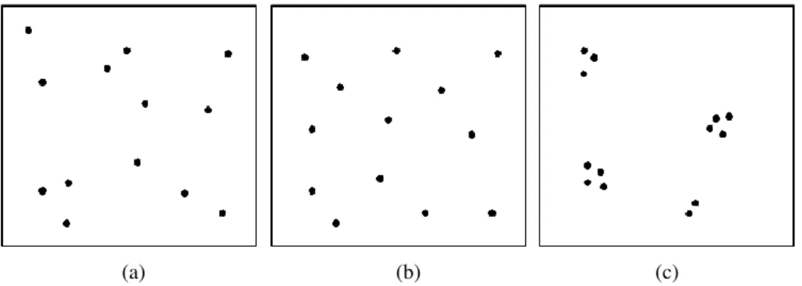
To illustrate, spatial configurations can be classified as random, regular or clustered.

A random classification can be defined when players are at random distances from each other

in the field, regular, when players are equally distant from each other in the field, or

clustered, when we can identify different groups of players aggregated in different parts of

(38)

38

interpersonal distances, in particular the minimum interpersonal distance, or nearest neighbor

distance (Clark, & Evans, 1954).

(a) (b) (c)

Figure 7: Example of spatial distribution patterns (a) random, (b) regular and (c) clustered.

The spatial distribution of the players in a field, and hence the space that a players has

to act, is dependent on a large number of constraints that change continuously throughout a

game, being ball possession an obvious one. In principle, the attacker team normally tries to

free-up space while the defender team tries to tie-up space (McGarry et al., 2002, Gréhaigne,

Bouthier, & David, 1997). Therefore, in terms of nearness, it is expected that the

interpersonal distance between players is kept greater for the attacker team and smaller for

the defender team, which results in more space for the attack. This relationship was already

observed using surface area (Frencken, Lemmink, Delleman, & Visscher, 2011) and stretch

index variables (Bourbousson, Sève, & McGarry, 2010).

An alternative method to study the spatial relation established between players at each

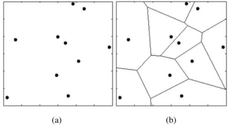
instant of a game is the Voronoi diagram (Dirichlet, 1850, Voronoi, 1908), which is a spatial

construction that allows a spatial partition of the field area into cells, each associated to each

of the players, according to their positions (Figure 8). These cells result from applying a very

simple nearest-neighbor rule: each player, represented by the coordinates of his/her location

in the field, is associated to all parts of the field that are nearer to that player than it is to any

(39)

39

(a) (b)

Figure 8: Example of a Voronoi diagram generated for the set of points represented in the figure.

Voronoi diagrams have already been suggested by other authors in the study of

players’ spatial distribution in team sports and to define players’ and teams’ dominant

regions, having been applied in a variety of game settings, namely, real soccer games (Taki,

Hasegawa & Fukumura, 1996), electronic soccer games (Kim, 2004), robotic soccer (Law,

2005) and real hockey games (Fujimura & Sugihara, 2005). When real games were

considered, dominant regions were calculated considering more than just players’ location, in

particular, Taki, Hasegawa & Fukumura (1996) has considered players’ direction and speed,

whereas Fujimura & Sugihara (2005) has taken into account players’ distance from ball and

distance to goal. In all these studies it was shown that the position of the ball influences the

location of the players and hence the size of their respective dominant regions.

Besides the advances of the work mentioned above towards the analysis of spatial

patterns of behavior in team sports, an important dimension has not been considered. In fact,

when analyzing systems of interacting agents, it is necessary to measure its degree of

complexity (Stergiou, Buzzi, Kurz, & Heidel, 2004, Harbourne, & Stergiou, 2009), as this is

a key issue to understand the emergence of successful performances in dynamical movement

systems (Bartlett, Wheat & Robins, 2007, Davids, Glazier, Araújo, & Bartlett, 2003). To

assess the complexity of a system, one can consider a nonlinear measure suggested by Pincus

(40)

40

signal from a variable measured in the system under study. When this variable expresses the

state of the system (Harbourne, & Stergiou, 2009), its regularity is directly proportional to the

system’s complexity, i.e., lower values of ApEn indicate more regularity and hence low

complexity.

Thus, the main goal of the present paper was to characterize the spatial interaction

dynamics of players in team sports, by understanding how players from two opposite teams

coordinate their location in the field during a game and how they define and adjust their

dominant regions throughout the game. We expect that players from the attacker team present

greater interpersonal distances, greater dominant regions, and greater regularity overtime in

terms of space area as they are with the ball.

Material and Methods

In this study were considered 19 experimental plays of Futsal, in which participants

were 15 male senior players (23.25 ± 1.96 years old), treated in agreement with the ethical

standards of American Psychological Association (APA). Plays represent the sub-phase of

Futsal of 5 vs 4+GK performed in half field (20 m width × 20 m depth) where all players

occupied fixed initial positions. This is a common scenario in Futsal when the team losing the

game has ball possession and aims to score where, due to numerical disadvantage, the

defender team retract their positions to their half field. Accordingly, in each play, the aim of

the attacker team is to score while the defender team tries to avoid it, and each play ends

whenever the attack loses ball possession.

Two fixed digital video cameras at 25 Hz were used to capture players’ movements

during each play. The trajectory of each player was extracted from the recorded videos using

(41)

41

transformed into real coordinates (x,y) using a direct linear transformation method (2D-DLT)

(Abdel-Aziz, & Karara, 1971). The 19 plays had, on average, 848 (± 374) frames

(corresponding to approximately 34.2 (± 14.94) seconds), minimum of 315 and maximum of

1558 frames (approximately 12.6 and 62.4 seconds, respectively).

In the present work two variables were considered to describe this system, players’

dominant region, as defined by the respective Voronoi cell, and the minimum interpersonal

distance between teammates. The minimum interpersonal distance between all teammates

(N), here designated nearest teammate distance (DistNT), was calculated at each frame (f),

considering the Euclidean distances between all pairs of players of a team (A), as described

below.

{

x_if x_jf y_if y_jf

}

i j N j

i j i

f _min ₍ ₎ ₍ ₎ _, _, ₁_,..., )

(A

Dist 2 2

,

NT = − + − =

≠

As for players’ individual dominant region, we considered the respective Voronoi

cells and calculated their area (AreaDR) as described next.

The field was mapped with a grid of 20×20 positions. At each frame (f), the area of

the DR of player k (k∈[1,M]) is the sum of all grid positions (i,j) (where i=1,..,20 and

j=1,…,20) that are closer to that player than it is to any other player. This can be

mathematically defined as presented below,

M k I i j j i f ,.., 1 ) (k Area 20 1 20 1 ) , ( DR

∑∑

= = = =

where I(i,j) is a Boolean function that takes value 1 if player k is the closest player to

(42)

42

  

 ₋ ₊ ₋ _< ₋ ₊ ₋ _∀ _≠ ₌

= otherwise 0 ,.., 1 , , ) ( ) ( ) ( ) ( if

1 2 2 2 2

) , ( M m k m y j x i y j x i I f m f m f k f k j i

Grid points that are equidistant to two or more players constitute the boundaries of

their respective regions and therefore are not added to the corresponding areas.

For each player and team we investigated how the size of their dominant regions

changes over time and how the size of such regions relates to each other. MATLAB routines

were written to generate, at each frame, the Voronoi diagram associated to the spatial

distribution of the players, and to calculate the size of the dominant region (AreaDR)

according to descriptions above.

The regularity of time series data from AreaDR and DistNT was measured using the

ApEnRatioRandom (Fonseca et al., 2012), which is a normalized measure of Pincus (1991)

approximate entropy (ApEn), obtained by dividing the ApEn of the original series, Y, by the

average ApEn of 100 random series of the same size of Y. This measure allows the

comparison of entropy values calculated in series of varying lengths. A value of

ApEnRatioRandom of approximately 0.2 indicates regularity (high predictability), whereas 1

indicates low regularity (high unpredictability) (Fonseca et al., 2012).

We used descriptive statistics (Mean (M) ± Standard Deviation (SD)) and inferential

statistics (ANOVA, t-test and paired t-test) to compare the spatial behavioral complexity

between players, teams, and teams by play, respectively.

Reliability

From all the plays, one of them was randomly selected and the data trajectories of the

(43)

43

reliability using technical error of measurement (TEM) and coefficient of reliability (R),

respectively (Goto & Mascie-Taylor, 2007). The TEM yielded values of 0.137 meters

(0.23%) and the coefficient of reliability was equal to 0.984.

Results

When looking at changes on the minimum interpersonal distance between teammate

players (DistNT) and area of the dominant region (AreaDR) across each play, we found that, on

average, players from the attacker team tend to be further from each other in comparison with

players from the defender team, as expected (Figure 9: exemplar single play). Consequently,

the space occupied by each player is, on average, greater for the team with the ball (attacker

team) in comparison with the defender team (Figure 10: exemplar single play).

(44)

44

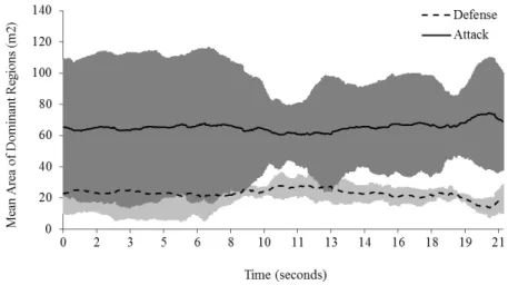
Figure 10: Mean area of the dominant region, across time, for the attacker and defender teams in a randomly selected play (error bars represent the standard deviation).

When comparing the amount of variability within each team for both variables, it is

clear that the attacker team shows less variability than the defender team in the DistNT and

more variability than the defender team in the AreaDR, as shown by the error bars in Figure 9

and Figure 10, respectively, This tendency was observed in all plays, suggesting that, in

comparison to what was found in the defender team, the area occupied by the attacker team is

much more variable within each frame, whereas the minimum interpersonal distance is less

variable. In Figures 9 and 10, the moment captured at time 10 s. corresponds to the exact

moment (observed by visual inspection) when the ball is received by an attacker inside the

defensive structure, which is, according to Futsal’s literature, a critical occurrence for the

defender team (Lucena, 2007). As a consequence, all defenders were trying to close the

space around the ball carrier and avoid the attacker team to score, and both DistNT and

AreaDR, presented particularly low variability.

To better understand and characterize the system under study, we measured the

regularity of DistNT and AreaDR, at both player and team levels and within each play, using a

normalized measure of the ApEn due to presence of signals with varying lengths (for more

(45)

45

calculated separately for each player in all plays. We found that the regularity of both

variables is significantly different between at least two players (DistNT: F(9,180)=9.5,

p<0.001; AreaDR: F(9,180)=12.5, p<0.001), being this difference only found between

opponent players. This means that players within a team have similar behavioral patterns

regarding proximity to their teammates and management of their dominant regions. At a team

level, the regularity of the same two variables was compared between the teams (Defender vs

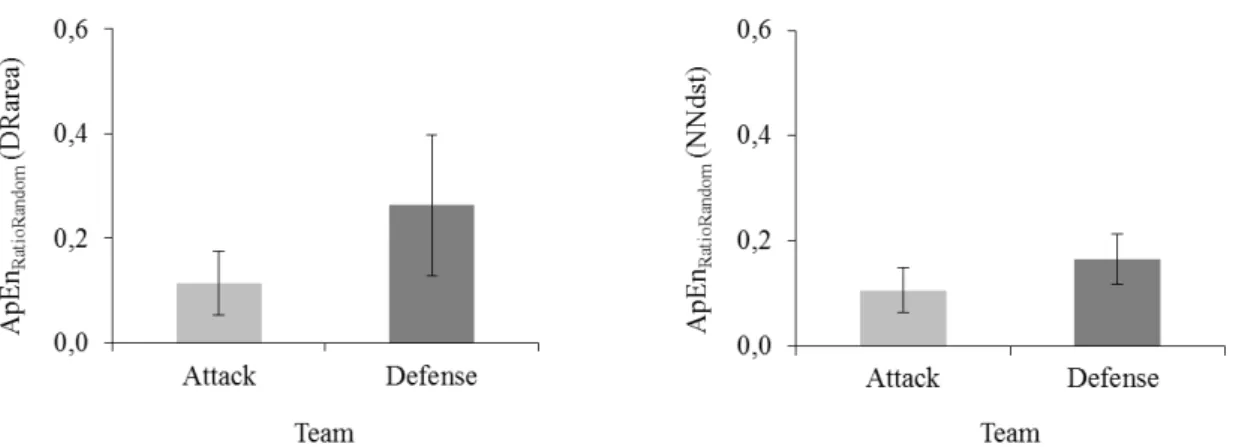
Attacker) and significant differences were found in both variables (DistNT: 0.165 ± 0.048 vs

0.106 ± 0.043, p<0.001; AreaDR: 0.264 ± 0.135 vs 0.114 ± 0.061, p<0.001). In addition, and

having shown a team effect, we tested the effect of the play in the spatial interacting behavior

between teams. Hence, for the same two variables, we considered, for each play and for each

team, the median entropy. Our results were consistent with what was shown above,

suggesting that, within a play, DistNT and AreaDR were significantly more regular for the

attacker team in comparison with the defender team ( t(18)=8.26, p<0.001; t(18)=8.86,

p<0.001, respectively) (Figure 11).

Figure 11: Comparison of the mean entropy of the distance to nearest teammate (DistNT) and area of the dominant region (AreaDR) between teams in the same play. Error bars represent the standard deviation

(*** p<0.001).

Discussion

The aim of this study was to characterize the spatial dynamics of players and teams in