1D and 2D Fourier-based approaches to numeric
curvature estimation and their comparative
performance assessment
Leandro Farias Estrozi,
aLuiz Gonzaga Rios-Filho,
aAndrea Gomes
Campos Bianchi,
aRoberto Marcondes Cesar Jr.,
band
Luciano da Fontoura Costa
a,∗aCybernetic Vision Research Group, IFSC-USP, Caixa Postal 369, São Carlos, São Paulo, 13560-970, Brazil bCreative Vision Research Group, Department of Computer Science, IME, University of São Paulo,
Rua do Matão, 1010, São Paulo, 05508-900, Brazil
Abstract
A careful comparison of three numeric techniques for estimation of the curvature along spatially quantized contours is reported. Two of the considered techniques are based on the Fourier transform (operating over 1D and 2D signals) and Gaussian regularization required to attenuate the spatial quantization noise. While the 1D approach has been reported before and used in a series of applications, the 2D Fourier transform-based method is reported in this article for the first time. The third approach, based on splines, represents a more traditional alternative. Three classes of parametric curves are investigated: analytical, B-splines, and synthesized in the Fourier domain. Four quantization schemes are considered: grid intersect quantization, square box quantization, a table scanner, and a video camera. The performances of the methods are evaluated in terms of their execution speed, curvature error, and sensitivity to the involved parameters. The third approach resulted the fastest, but implied larger errors; the Fourier methods allowed higher accuracy and were robust to parameter configurations. The 2D Fourier method provides the curvature values along the whole image, but exhibits interference in some situations. Such results are important not only for characterizing the relative performance of the considered methods, but also for providing practical guidelines for those interested in applying those techniques to real problems.
2002 Elsevier Science (USA). All rights reserved.
*Corresponding author.
E-mail addresses:[email protected] (L.F. Estrozi), [email protected] (L.G. Rios-Filho), [email protected] (A.G. Campos Bianchi), [email protected] (L.F. Costa).
Keywords:Digital signal processing; Curvature estimation; Differential geometry; Numerical methods; Fourier transform; Shape analysis; Performance assessment; Gaussian regularization
1. Introduction
The analysis of 2D shapes is one of the most classical, important, and widely studied problems in pattern recognition and computer vision, finding applications in a myriad of practical problems. Nevertheless, in spite of its seeming simplicity, there is no definitive approach to 2D shape analysis and classification, and much effort is still needed mainly in order to assess the existing techniques and to improve the accuracy and recognition rates of the most reliable approaches. Among the different methods for 2D shape analysis, those based on the shape boundarycurvatureconstitute some of the most comprehensive and promising, as discussed in more detail in the following. The main objectives of the present article are twofold: to introduce a new Fourier-based 2D curvature estimation technique and to comparatively evaluate the performance of three numerical methods for digital curvature estimation. Such results can provide valuable insight not only on the specific advantages and disadvantages of each method, but at the same time offer practical guidelines for those interested in applying the techniques in real problems. In addition, the adopted performance assessment framework can be generalized to other curvature estimation techniques.
First, as far as information preservation is concerned, curvature is a complete represen-tation, since the original curve can be reconstructed (up to rigid-body transformations). Furthermore, since it is a well-accepted fact that not all points on shape boundaries are equally relevant, finding the more salient (or critical) points is an extremely important task for feature extraction and contour segmentation. Curvature also plays a central role within this context: there are various methods that search for these critical points in terms of local maximum and minimum curvature points, as well as zero curvature (straight line) por-tions. The curvature is invariant to rigid-body transformations (i.e., translations, rotations, and reflections). In addition, psychophysical evidences have also shown that curvature is an extremely important cue for our visual perception processes [1], in such a way that cur-vature peaks tend to correspond to the salient shape points. Finally, interesting physical analogies based on the curvature concept have led to powerful shape analysis techniques. For instance, elasticity theory provides the useful concept ofbending energy, a global fea-ture calculated in terms of the curvafea-ture along the contour [2,3], which can be used for characterizing shape complexity [4].
can be easily smoothed in the Fourier domain and that the Fourier descriptors, which are valuable resources for the shape characterization and classification, are obtained as byproducts.
Basically, there are two different ways of estimating the curvature of a digital shape, i.e., either from the object parametrized outline or directly from the 2D image by using the concept of isopotential curves. Contour-based approaches are more popular and widely used in different vision problems such as in biomedicine, fingerprint recognition, and OCR [11–13], presenting several interesting advantages such as the fact that dealing inherently with 1D data representations is computationally less demanding and the existence of substantial technical literature on contour analysis [7].
Nevertheless, one of the main drawbacks of this approach is the fact that the object must have its contour extracted in parametric fashion before further analysis [7]. On the other hand, the latter class of techniques, which is applied directly to the 2D image, does not depend on contour tracking, allowing dedicated hardware to be used to implement the imaging procedures (such as convolution). Furthermore, the size of the input data becomes independent of the object perimeter, which does not hold to the contour-based approach, since the number of points of the extracted contour varies with the object perimeter. A good discussion on the robustness of computing derivatives over a level set can be found in [14]. The reader is referred to [15–18] for a detailed review of the many alternative curvature estimation methods for digital images. The main problem that must be solved for digital curvature estimation is that the curvature expression involves differentiation of discrete data, which is an ill-posed problem that must be circumvented by the introduction of a regularization procedure. The standard approach is based on smoothing the data, e.g., by convolving the contour with a gaussian kernel, which is the case, for instance, in the now classical work of Mokhtarian and Mackworth [19]. Alternative approaches include local interpolation of the data [6] and the use of different discrete curvature measures, such as the c-curvature of Davis [20]. On the other hand, the 2D-based techniques have also received attention from the image processing community. Some examples of works devoted to this approach can be found in [21,22].
Another important aspect addressed in the present work concerns the validation and comparison of the 1D and 2D Fourier-based approaches. Indeed, vision science researchers have been criticized not only for not spending enough attention on characterizing the performance of new approaches respectively to a representative set of data, but also for not comparing such new techniques with a more traditional alternative [23,24]. Only more recently have some works addressed the topic of performance assessment in a systematic way [25–28]. One of the main characteristics of the present work is to go a long way toward addressing these criticisms. First, special care is spent in trying to define a representative set of data (see Section 3.1), with special attention given to 2D closed, simple (in the sense of being Jordan curves) parametric curves. The reason for concentrating on closed curves is that this type of curve is inherently compatible with Fourier-based derivative estimation. In other words, the fact that both these curves and the discrete Fourier transform are periodical allows continuity of the curve and its derivatives, which is not generally verified for open curves.
large, even if not completely representative, set of shapes than to consider just a handful, as sometimes happens in the related literature. More specifically, three kinds of curves have been considered: (a) those defined by analytical expressions, such as sinusoidal circles and spirals; (b) curves defined by B-splines [5]; and (c) curves synthesized in terms of spectral content [29]. It is important to note that, in each of these cases, it is possible to obtain an analytical and absolutely precise quantification of the point curvature along the contours (see Section 3.2), to be used as a standard for comparison. Each of these is spatially sampled, before numeric estimation, according to four quantization schemes: (i) grid-intersect quantization, (ii) square box quantization, (iii) using a conventional camera, and (iv) using a conventional scanner. Observe that (iii) and (iv) also involve printing the shapes through a conventional laser printer. These two latter schemes provide a more global characterization of the considered methods given typical practical situations.
Great attention has also been focused in defining unbiased and comprehensive merit figures allowing proper characterization of the considered techniques (see Section 3.3). The important features to be considered included the accuracy in the curvature calculation, defined in terms of root mean square (RMS) error between the analytical and numerically estimated curvatures, the robustness to parameter tuning, expressed in terms of the distribution of the optimal parameters (the scale parameters defined by the standard deviation of the smoothing Gaussians), and the execution time. A more detailed discussion of such measures can be found in Section 4.
In addition to trying to characterize the performance of the considered techniques according to a formal, comprehensive, and comparative fashion, there are some particularly interesting questions, inherently defined by the specific features of the Fourier techniques, which should at least partially be answered by the considered framework. For instance, since both first and second order derivatives are needed in the 1D and 2D approaches, it would be interesting to verify the use of two distinct standard deviation values in the regularizing Gaussian smoothing. In other words, since the second order derivatives imply higher enhancement of high frequencies than those needed for first order derivatives, it is interesting to check whether the use of a larger smoothing for the second derivative would lead to improved accuracy. Another important point to be investigated concerns the robustness of the techniques given different parameter settings.
The current article starts by describing the three curvature estimation numerical approaches considered, covering the 2D Fourier-based approach (first outlined in [30]) in more detail. Then, the performance assessment framework is presented in detail, which is followed by the obtained results and the respective discussion. The paper concludes by presenting the overall conclusions as well as possibilities for future developments.
2. Fourier-based curvature estimation
quasi-unitary, lies in the fact that the complex exponential basis used in this transformation, because of its highly correlated nature, usually allows the signal to be represented in a much more compact form, i.e., with just a few spectral components. However, the Fourier transform also possesses a series of additional interesting properties, such as the differentiation property, given by Eqs. (1) and (2), respectively, to 1D and 2D signals, where H (f )= ℑ(h(t)) andH (u, ν)= ℑ(h(x, y)). Such properties allow an interesting means for numeric estimation of derivatives, since the Fourier transform can be fast and effectively performed numerically
dn
dtnh(t)= ℑ
−1
(i2πf )nH (f )
, (1)
∂n ∂xn
∂m
∂ymh(x, y)= ℑ
−1
(i2π u)n(i2π v)mH (u, v)
, (2)
wherei=√−1 . Given that curvature has a differential nature, as it is clear from Eq. (3), it is in principle possible to use the properties (1) and (2) as a means for numerical estimation of curvature. Observe that thexandyvariables in Eq. (3) refer to the parametric functions x(t) andy(t) defined by the contour. Initially proposed in [31], in terms of Fourier series and Kaiser regularizing windows, this possibility has been more extensively developed and applied in a more recent series of developments [7–9] and which rely on the Fourier transform and Gaussian smoothing, being essential for regularizing the high frequency noise introduced by the spatial quantization. Indeed, the standard deviation of the regularizing Gaussian defines a scale parameter allowing multiresolution representation of the estimated curvature [8,9]. While such works focused curvature estimation of 2D closed contours, done in terms of 1D Fourier transform, it is also interesting to investigate the possibility of using 2D Fourier transform. The main advantage of such an approach is that it can be applied to estimate the curvature, by using Eq. (4), alongallthe isopotential curves defined by a surfaceφ(x, y)containing the original shape contour as one of its level curves, which can be done. A secondary advantage of such an approach is that the size of the input data does not necessarily vary with the perimeter of the shapes, as happens in the 1D approach.
k= x˙y¨− ˙yx¨
(x˙2+ ˙y2)3/2, (3)
k= ∇ · ∇φ
∇φ =
φxxφy2−2φxφyφxy+φyyφx2
(φx2+φy2)3/2 . (4)
The next sections present the 1D and 2D Fourier-based curvature estimation techniques, respectively, with special attention given to the latter, since it is presented here for the first time.
2.1. Curvature estimation based on parametric curve approximation
witht∈ [0,1], which approximates a curve segment between two contour pointsA (t=0) andB (t=1). Therefore, for this curve segment, the approximation curve is defined as:
x(t)=a1t3+b1t2+c1t+d1, (5)
y(t)=a2t3+b2t2+c2t+d2. (6)
By calculating the respective derivatives and substituting them in the curvature expression, Eq. (3), it can be easily verified that the curvature at the pointA (t=0)of the contour is
k=2c1b2−c2b1
(c12+c22)3/2. (7)
Medioni and Yasumoto [6] have used cubic B-splines with equally spaced nodes for piecewisely adjusting the parametric curve segments. The coefficientsb1,b2,c1, andc2
of Eq. (7) above can be calculated, from the above expressions, as (refer to [6] for further detail):
b1=121
(xn−2+xi+2)+2(xn−1+xn+1)−6xn, (8)
b2=121(yn−2+yn+2)+2(yn−1+yn+1)−yn
, (9)
c1=121(xn+2−xn−2)+4(xn+1+xn−1), (10)
c2=121(yn+2−yn−2)+4(yn+1+yni−1). (11)
The curvature is calculated by substituting the above coefficients in the curvature equa-tion (7).
2.2. 1D curvature estimation based on the fourier derivative property
The curvature estimation method discussed in this section originates from the curveg-ramconcept discussed in [8,9] and has been considered in several applications [4,7,10]. Let c(n)=(x(n), y(n))be the parametric contour of interest, withn=0, . . . , N−1, and let N be the number of points along the boundary. The contour can be represented as a com-plex signalu(n)=x(n)+iy(n). A fundamental tool for this approach is the 1D Fourier transform pair ofu(n), given by
U (s)= ℑu(n)= N−1
n=0
u(n)e−i2π (sn/N ), s=0, . . . , N−1, (12)
u(n)= ℑ−1U (s)= 1 N
N−1
s=0
U (s)ei2π (sn/N ). (13)
The auxiliary function η(s)is a useful tool for the estimation of the discrete derivatives ofu(n),
η(s)=
s, ifs=0,1, . . . ,N−floor(N/2)−1 , N−s, ifs=
N−floor(N/2) ,
N−floor(N/2)+1
with floor(N/2)being the truncation function. Functionη(s) implements the necessary alignment because of the representation normally produced by the DFT (i.e., the frequency representation formed by the second part followed by the first part of the next period). The signals should be smoothed because of a high frequency enhancement effect produced by numerical differentiation, which is achieved by taking the smoothed version u(n, a) ofu(n),
u(n, a)= ℑ−1
U (s)Ga(s), (15)
where Ga(s)=exp(−(aη(s))2). Contour shrinking is avoided by taking for the spatial scale parameter a a value as small as possible in order to filter the spatial quantization noise and not distort the contour too much. The smoothed first and the second derivatives ofu(n)are defined as
˙
u(n, a)= ℑ−1
i2π η(s)U (s)Ga(s), (16)
¨
u(n, a)= ℑ−1
−(2π η(s))2U (s)Ga(s). (17)
The multiscale curvature description ofu(n)is given by
k(n, a)=−ℑ{ ˙u(n, a)u¨
∗(n, a)}
| ˙u(n, a)|3 , (18)
wherez∗denotes the complex conjugate and|z|denotes the complex modulus ofz. Although it is possible to apply the 1D Fourier method to contours with any amount of points, it is often much more efficient to consider the number of points which are integer powers of two, because this situation allows for fast Fourier transforms. This can be easily accomplished by linearly interpolating the parametric curves along evenly distributed portions of the original curve, in order to produce a new representation with the desired amount of points, i.e., the smallest integer power of two larger than the original number of points.
2.3. 2D Fourier-based method
can also smooth the more abrupt transition implied by scheme (i). In order to favor speed and minimize curve interferences, the present article has adopted the former scheme. Once such an extensionφ(x, y)is achieved, the curvature of the contour defined byφ(x, y)=a (a level-curve) can be estimated by using Eq. (4) implemented in the Fourier domain considering Eq. (2).
As with the 1D approach described in the previous section, it is necessary to regularize φ(x, y), since it is represented in a spatially sampled space. This will be done by convolvingφ(x, y) with a circularly symmetric 2D Gaussian given by Eq. (19), which is more effectively done in the Fourier domain,
Gσ(x, y)= 1 2π σ2e−
(x2+y2)/2σ2. (19)
It should be observed that, though initially all the original contour points lie at the same level-curve, this is no longer true after the regularization. Since for small smoothing degree the curves do not shift too much, the curvatures are henceforth taken at the original coordinates.
3. The evaluation framework
In order for different numerical methods to be properly compared, it is important to define an overall computational framework which is as fair and comprehensive as possible. This endeavor entails three main issues, namely defining a suitable set of test shapes, modeling the spatial quantization schemes, and identifying suitable merit figures which can express how the methods fulfill the principal properties expected of them. The following sections present and discuss each of these issues, respectively.
3.1. The considered shapes
Fig. 1. Sinusoidal circles with varying number of branches and internal radiuses.
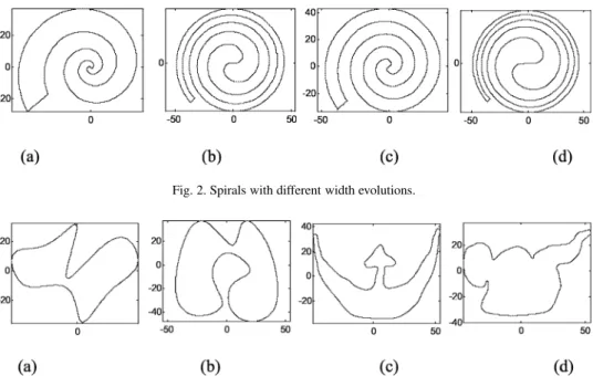
Fig. 2. Spirals with different width evolutions.
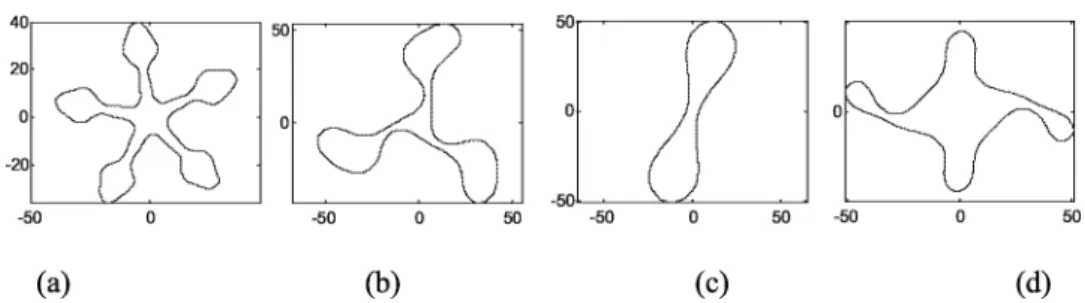
Fig. 3. Some of the considered B-spline-generated contours.
Fig. 4. Fourier synthesized shapes with different periods and harmonic compositions.
3.2. Spatial quantization schemes
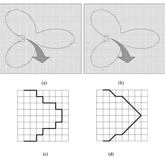
Considering that the selected shapes have to be continuous in order to allow exact curvature quantification to be used as a comparison standard, it is necessary to use some suitable spatial quantization method, which maps such continuous curves into the orthogonal grid inherent to any digital image. Four distinct traditional quantization schemes have been considered in the present work in order to provide a general view of the performance of the numerical techniques under varying quantization conditions. Out of these four methods, two are precisely defined in mathematical terms: the grid intersect quantization [32], GIQ, and the square box quantization [32], SBQ. The other two quantization schemes consist of using a standard table scanner (HP Scanjet 4L) and a video camera (Sony CCD IRIS) in order to acquire the images of high quality printouts of the shapes (HP LaserJet 4L, 300 dpi). Figure 5 illustrates the GIQ (a) and SBQ (b) representations of a same shape, and zoomed respective sections (c) and (d). Since the SBQ typically implies a more dense spatial quantization of the original analytical curve, it could be expected that smaller errors would be obtained by a numerical curvature estimation technique operating over such representations.
It should also be observed that the GIQ and SBQ schemes can produce representations including double points, such as that marked with an∗in Fig. 6a. Since such double points can make the curve not regular during curvature estimation, it is important to remove them, which is currently done by incorporating additional conditions in the curve quantization.
Special remarks regarding the detection of the shape edges include the fact that, while this operation is not required when considering the GIQ and SBQ schemes, a simple thresh-old operation followed by binary edge detection is considered for the shapes obtained from the scanner and camera. In practical general situations, traditional edge detection schemes (see, for instance, [7,33,34]) can be applied. The slightly different edges obtained by such different methods are uniformized by the Gaussian smoothing inherent to the application of different contour extraction algorithms that generally affect curvature estimation [35].
3.3. Merit figures
Fig. 5. Square box (a) and grid intersect (b) quantizations of a specific parametric curve, and respective zoomed sections (c) and (d).
to each numerical method and comparing the analytical and the numerically estimated cur-vatures along the curve. As already observed, three performance characteristics have been specially taken into account: (a) the implied execution times, (b) the estimation errors, and (c) the sensitivity of the techniques given specific parameter configurations, here quantified in terms of the dispersion of the optimal scale parameter values and the extension of the spatial scales for which the error does not exceed 10% of the minimal error.
One of the most direct and intuitive ways of quantifying the estimation error is in terms of some traditional metrics, such as the RMS error, an approach that is adopted in the present article. More specifically, for each shape and considered method, a global errorε is obtained by using Eq. (20), where ko is the calculated curvature using the proposed techniques,kais analytical quantized curvature, andN is the number of contour points.
εrms=
1 N N i=1
ko(i)−ka(i)2. (20)
However, while the Euclidean distance does provide a global measurement of similarity between all the original and estimated curvatures along the curves, it also presents some shortcomings. For instance, a large difference in just a single point may generally influence the overall error. Since such problems will be implied by virtually any alternative metric, we tried to control such effects by having the curvatures (both analytical and numerical) equalized through a sigmoid function (thus limiting curvature values within the[−3,+3] range) before the Euclidean distance is calculated. This process involves Eq. (21), wherex denotes a curvature value andais the maximum allowed curvature absolute value.
S(x)=a
ex/a−e−x/a
ex/a+e−x/a
=a
1− 2 e2x/a+1
. (21)
In order to provide a more complete characterization of the estimation error, the Euclidean distances have been organized in terms of histograms.
Fig. 7. Spatial scale extension considered as a sensitivity quantitative measure.
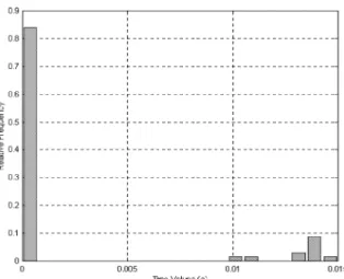
Fig. 8. Time histogram for interpolated version of the 1D Fourier method. Average value (standard devi-ation)=0.008(±0.003)s.
4. Results
Fig. 9. Time histogram for the 2D Fourier method. Average value (standard deviation)=3.5(±0.2)s.
Fig. 10. Time histogram for Medioni and Yasumoto’s method. Average value (standard deviation) = 0.002(±0.005)s.
were obtained by running Delphi (versions 3 and 4) implementations of the techniques in a Pentium II 333 MHz, 256 Mbytes of memory, IBM-PC compatible microcomputer under Windows 95.
4.1. Execution times
(a)
(b)
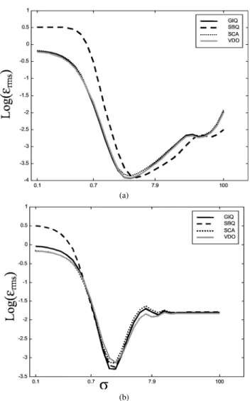
Fig. 11. Typical behavior of the estimation error for 1D (a) and 2D (b) Fourier-based methods. Both scales are logarithmic.
strategy allows the fastest execution speeds through the FFT. It should be observed that the presented histograms include all the considered curve classes and quantizations. The time required to linearly interpolate the curves in the 1D Fourier approach (explained in Section 2.2) has not been considered in the execution times. When interpolated, the great majority of the curves resulted in 1024 points.
4.2. Histograms of curvature estimation errors
(a)
(b)
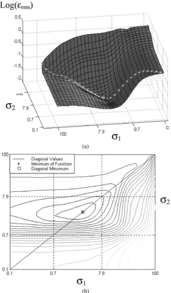
Fig. 12. Typical errors obtained for curvature estimation considering a series of combinations of the regularizing parametersσ1andσ2. Situation where the minimal error lies on the main diagonal.
to verify the possible improvements allowed by using two distinct values of standard deviations, σ1 and σ2, respectively, as regularizing parameters for the first and second
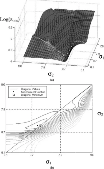
derivatives (see Section 1), the Fourier-based methods were run for several combinations of such scale parameters. Figures 12 and 13 present typical results, with respect to the B-spline in Figs. 3b and 1c. These two figures illustrate the situations where the minimum error lies on and off the main diagonal.
(a)
(b)
Fig. 13. Typical errors obtained for curvature estimation considering a series of combinations of the regularizing parametersσ1andσ2. Situation where the minimal error lies off the main diagonal.
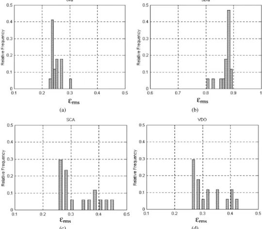
standard deviation; i.e., σ1=σ2. Figures 14–16 present the histograms of errors with
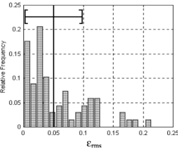
Fig. 14. Curvature estimation errors for the 1D Fourier-based curvature technique, without interpolation. Average value (standard deviation)=0.05(±0.04).
Fig. 15. Curvature estimation errors for the 2D Fourier-based curvature technique. Average value (standard deviation)=0.05(±0.05).
4.3. Parameter sensitivity
Fig. 16. Curvature estimation errors for Medioni and Yasumoto’s approach. Average value (standard deviation)=0.4(±0.2).
(a) (b)
(c) (d)
Fig. 18. Histogram of the dispersion of the spatial scale parameter (standard deviation) values for the 1D Fourier-based method (without interpolation).
Fig. 19. Histogram of the dispersion of the spatial scale parameter (standard deviation) values for the 2D Fourier-based method.
portions of the curve that, although close in the 2D space, are further away along the perimeter.
5. Discussion
Fig. 20. Histogram of the extension of the spatial scale ensuring error not larger than 10% of the minimal error, for the 1D Fourier technique.
Fig. 21. Histogram of the extension of the spatial scale ensuring error not larger than 10% of the minimal error, for the 2D Fourier technique.
between the different classes of curves, which is a desirable feature substantiating the method robustness. As indicated in Figs. 18 and 19, the optimal values ofσ of more than 70% of the curves are contained in the interval[1.5, 4]. Regarding the other considered sensitivity parameter, namely the spatial scale extension (see Fig. 7), about 80% of all cases processed by the 1D and 2D Fourier techniques (see Figs. 20 and 21) presented an extension larger than 10 pixels, indicating robustness with respect to the choice ofσ.
considered in the Fourier approaches. Other general observed tendencies included the fact that the 1D approach considering the linear interpolation outlined in Section 2.2 provided much faster execution time than the 2D method and the 1D approach without interpolation, which is a direct consequence of the use of the fast Fourier transform. On the other hand, similar estimation errors and sensitivity to parametric configurations were obtained for these two techniques (see Fig. 11). It should be also observed that while the speed of the 2D approach depends on the size of the rectangle involving the curve, the execution time of the 1D approach is defined by the perimeter of the curve. A particularly interesting phenomenon, henceforth called interference, has been observed for the 2D Fourier approach. As is clear in Fig. 22, curves containing bottlenecks, i.e., portions which are close in the 2D space but distant along the perimeter, tend to produce error peaks. This has been verified to be a consequence of the fact that the convolution mask comprehends, especially at larger scales, not only the neighborhood of the point where the differential operators are being estimated, but also points from the other portion of the curve. The position of such error peaks is consequently determined by the bottleneck spatial scale. It should be observed that this phenomenon does not imply a shortcoming for curvature estimation, since it occurs at spatial scales much higher than that respective to the optimal error, but can undermine scale space representations derived by the 2D approach.
Little performance variation has been observed with respect to the three classes of curves and quantization schemes—which indicates that the GIQ and SBQ are good models for the sampling implied by standard scanners and video cameras (see Fig. 11), at least as far as curvature estimation is concerned. An exception has been verified for Medioni and Yasumoto’s approach, where the SBQ has implied a much larger error than the other quantizations (Fig. 17), since the SBQ produces more jagged contours (Fig. 5). However, in the case of the Fourier methods, the SBQ often accounted for better accuracy, as a possible consequence of the richer representation of the curve allowed by this quantization scheme.
6. Concluding remarks
Generally speaking, Medioni and Yasumoto’s approach is particularly suited for situations demanding very fast execution time, but not critical in terms of accuracy. This is in great part a consequence of the fact that this method does not include any resource for filtering out the spatial quantization noise. On the other hand, the Fourier-based schemes account for particularly interesting alternatives for applications requiring very low estimation errors. Moreover, the 1D Fourier approach is faster than the 2D, but the latter has the advantage of allowing the curvature to be estimated not only along the original contour, but throughout its 2D extension, which can be particularly useful in situations involving curvature estimation for the numerical solution of partial differential equations [14]. The interesting phenomenon of interference has also been observed for the 2D Fourier approach. By characterizing in quantitative terms the advantages and disadvantages of the considered methods, as well as indicating suitable choice of the respective parameters, the obtained results also provide valuable guidelines for those interested in applying the considered techniques in real problems.
Acknowledgments
Luciano da Fontoura Costa is grateful to FAPESP (Procs 99/12765-2) and CNPq (Procs 301422/92-3 and 468413/00-6) for financial support. Roberto M. Cesar Jr. is grateful to FAPESP for the financial support (98/07722-0), as well as to CNPq (300722/98-2). Andrea Gomes Campos and Luiz Gonzaga Rios-Filho are grateful to FAPESP (Procs 98/12425-4 and 98/13427-0, respectively). Leandro Farias Estrozi is grateful to CAPES.
References
[1] F. Attneave, Some informational aspects of visual perception, Psych. Rev. 61 (1954) 183–193.
[2] I.T. Young, J.E. Walker, J.E. Bowie, An analysis technique for biological shapes I, Inform. Control 25 (1972) 357–370.
[3] J.E. Bowie, I.T. Young, An analysis technique for biological shapes II, Acta Cytol. 21 (1972) 455–464. [4] R.M. Cesar Jr., L. da F. Costa, The application and assessment of multiscale bending energy for
morphometric characterization of neural cells, Rev. Sci. Instr. 68 (1997) 2177–2186. [5] M.E. Morteson, Geometric Modelling, Wiley, New York, 1985.
[6] G. Medioni, Y. Yasumoto, Corner detection and curve representation using cubic B-splines, Comput. Vision Graphics Image Process. 39 (1987) 267–278.
[7] L. da F. Costa, R.M. Cesar Jr., Shape Analysis and Recognition: Theory and Practice, CRC Press, Boca Raton, FL, 2001.
[8] R.M. Cesar Jr., L. da F. Costa, Piecewise linear segmentation of digital contours in O(NLog(N ))
through a technique based on effective digital curvature estimation, Real-Time Imaging 1 (1995) 409–417, doi:10.1006/rtim.1995.1042..
[9] R.M. Cesar Jr., L. da F. Costa, Towards effective planar shape representation with multiscale digital curvature analysis based on signal processing techniques, Pattern Recog. 29 (1996) 1559–1569.
[10] L. da F. Costa, T.J. Velte, Automatic characterization and classification of ganglion cells from the salamander retina, J. Comp. Neurol. 404 (1999) 33–51.
[11] E. Persoon, K.S. Fu, Shape discrimination using Fourier descriptors, IEEE Trans. Systems Man Cybernet. 7 (1977) 170–179.
[13] S.A. Mahmoud, Arabic character recognition using Fourier descriptors and character contour encoding, Pattern Recog. 27 (1994) 815–824.
[14] J. Sethian, Level Set Methods: Evolving Interfaces in Geometry, Fluid Mechanics, Computer Vision, and Material Science, 2nd ed., Cambridge University Press, New York , 1999.
[15] D.P. Fairney, P.T. Fairney, On the accuracy of point curvature estimators in a discrete environment, Image Vision Comput. 12 (1994) 259–265.
[16] T. Pavlidis, Algorithms for shape analysis of contours and waveforms, IEEE Trans. Pattern Anal. Mach. Intell. 2 (1980) 301–312.
[17] S. Loncaric, A survey of shape analysis techniques, Pattern Recog. 31 (1998) 983–1001. [18] S. Marshall, Review of shape coding techniques, Image Vision Comput. 7 (1989) 281–294.
[19] F. Mokhtarian, A. Mackworth, A theory of multiscale, curvature based shape representation for planar curves, IEEE Pattern Anal. Mach. Intell. 14 (1992) 789–805.
[20] L.S. Davis, Understanding shapes: Angles and sides, IEEE Trans. Comput. 26 (1977) 236–242.
[21] C.H. Chen, J.S. Lee, Y.N. Sun, Wavelet transformation for gray-level corner detection, Pattern Recog. 28 (1995) 853–861.
[22] L. Kitchen, A. Rosenfeld, Gray-level corner detection, Pattern Recog. Lett. 1 (1982) 95–102.
[23] R.C. Jain, T.O. Binford, Dialogue: Ignorance, myopia, and naiveté in computer vision systems, Comput. Vision Graphics Image Process. Image Understanding 53 (1991) 112–117.
[24] M. Kunt, Dialogue: Comments on “Dialogue,” a series of articles generated by the paper entitled “Ignorance, myopia, and naïveté in computer vision,” Vision systems, Comput. Vision Graphics Image Process. Image Understanding 54 (1991) 428–429.
[25] J.L. Barron, D.J. Fleet, S.S. Beauchermin, Performance of optical flow techniques, Int. J. Comput. Vision 12 (1994) 43–77.
[26] K. Cho, P. Meer, J. Cabrera, Performance assessment through bootstrap, IEEE Trans. Pattern Anal. Mach. Intell. 19 (1997) 1185–1198.
[27] D. Demigny, T. Kamlé, A discrete expression of Canny’s criteria for step edge detector performances evaluation, IEEE Trans. Pattern Anal. Mach. Intell. 19 (1997) 1199–1211.
[28] M.D. Heath, S. Sarkar, T. Sanocki, K.W. Bowyer, A robust visual method for assessing the relative performance of edge-detection algorithms, IEEE Trans. Pattern Anal. Mach. Intell. 19 (1997) 1338–1359. [29] C.T. Zahn, R.Z. Roskies, Fourier descriptors for plane closed curves, IEEE Trans. Comput. 21 (1972) 269–
281.
[30] L.F. Estrozi, A.G. Campos, L.G. Rios, R.M. Cesar Jr., L. da F. Costa, Comparing curvature estimation techniques, in: Proc. 4th Simpósio Brasileiro de Automação Inteligente-SBAI, São Paulo, Brazil, 1999, pp. 58–63.
[31] M. Baroni, G. Barletta, Digital curvature estimation for left ventricular shape analysis, Image Vision Comput. 10 (1992) 485–494.
[32] H. Freeman, Computer processing of line-drawings images, Comput. Surv. 6 (1974) 57–95. [33] R.F. Gonzalez, R.E. Woods, Digital Image Processing, Addison–Wesley, Reading, MA, 1993. [34] R. Schalkoff, Digital Image Processing and Computer Vision, Wiley, Singapore, 1989.
[35] J.R. Bennett, J.S. Mac Donald, On the measurement of curvature in a quantized environment, IEEE Trans. Comput. 24 (1975) 803–820.
Leandro Farias Estrozi obtained his B.Sc. in physics from the Institute of Physics at the University of São Paulo, Brazil in 1998, and is currently a Ph.D. student in computational physics at the same institution. His research interests involve 2D and 3D shape analysis, the development of skeletonization algorithms and curvature estimation, psychophysical studies of saccadic vision, the development of tools for scientific visualization, and platforms for WWW-based psychophysical experiments. To find out more about his research and some selected publications take a look at http:// cyvision.if.sc.usp.br/~lfestroz.
and at aerospace industries. He participated twice in the Brazilian’s Antarctic Station Comandante Ferraz (King George Island) for the INPE. He is currently working on his Ph.D. thesis (Instituto de Física de São Carlos, University of São Paulo, Brazil), investigating the shape-function relationship in neural cells using mathematical models of the cells and of the extracellular medium. His research interests are computational neuroscience, neuromorphometry, computational and biological vision, image processing, and pattern recognition.
Andrea Gomes Campos obtained her M.Sc. in computational physics from the Insitute of Physics at the University of São Paulo, Brazil, on the subject of nonlinear edge detection techniques, where she is currently working toward her Ph.D. Her research interests are computer vision, image processing, pattern recognition, computational neuroscience, and neuromorphometry. Her main project is aimed at the characterization, modeling, and computational simulation of neurons considering internal and external factors that can influence their shapes.
Roberto M. Cesar Jr. received a B.Sc. in computer science (UNESP, Brazil), an M.Sc. in electrical engineering (UNICAMP, Brazil), and a Ph.D. in computational physics at the Institute of Physics, University of São Paulo, São Carlos, Brazil, including a period with the Departement de Physique of the Université Catholique de Louvain, Belgium. He held a post-doctoral position at the CVRG-Sao Carlos in 1997. He is currently a lecturer in the Department of Computer Science of IME-USP. His main research interests concentrate on several problems in the fields of computer vision, pattern recognition, and image processing.