Simulation of population size and genome saturation level for genetic
mapping of recombinant inbred lines (RILs)
Luciano da Costa e Silva
1, Cosme Damião Cruz
1, Maurilio Alves Moreira
2and Everaldo Gonçalves de Barros
11
Departamento de Biologia Geral, Universidade Federal de Viçosa, Viçosa, MG Brazil.
2
Departamento de Bioquímica e Biologia Molecular, Universidade Federal de Viçosa, Viçosa, MG, Brazil.
Abstract
Various population sizes and number of markers have been used to obtain genetic maps. However, the precise num-ber of individuals and markers needed for obtaining reliable maps is not known. We used data simulation to deter-mine the influence of population size, the effect of the degree of marker saturation of the genome, and the number of individuals required for mapping of recombinant inbred lines (RILs). Three genomes with 11 linkage groups were generated with saturation levels of 5, 10 and 20 cM. For each saturation level populations were generated with 50, 100, 154, 200, 300, 500 and 800 individuals with 100 replications for each population size. A total of 2100 populations was generated and mapped. Small marker numbers and small population sizes produced maps with more than 11 linkage groups. As population size and marker saturation increased, marker inversion and non-linked markers de-creased, moreover, between-marker distance estimates were improved. In this study, a minimum size of 200, 300 and 500 individuals were necessary for obtaining reliable maps when they were evaluated over the saturation levels of 5, 10 and 20 cM, respectively.
Key words:recombinant inbred lines, molecular markers, number of individuals, computer simulation.
Received: January 4, 2007; Accepted: April 27, 2007.
Introduction
In plant and animal breeding, genetic maps are impor-tant tools for analyzing genomes and dissecting complex traits into their simple Mendelian determinants. They also allow for identification of genome regions harboring genes controlling qualitative and quantitative traits (Lander and Botstein, 1989). However, availability of reliable maps de-pends on several factors such as the type and size of popula-tion and the type and number of markers. In addipopula-tion, other aspects must also be considered such as single loci segrega-tion ratio, recombinasegrega-tion frequency and logarithm of odds (LOD) thresholds used to infer linkage.
In plants, populations obtained from crossing two in-bred lines are commonly used for mapping, with the F2,
backcrosses (BC), Fn(n =3, 4,...,∞), double haploids (DH)
and recombinant inbred lines (RIL) being the most fre-quently used populations (Burret al., 1988). Alternatively, outbred populations such as half and full sibs can be used. The choice of the population depends on the species stud-ied, program goals and availability of time and funds.
A recombinant inbred line can be obtained from an F2
generation by successive self-pollinations using the single seed descent method (SSD) (Burret al., 1988). The resulting inbred lines are highly homozygous and the segregation ratio for each locus tends to 1:1 (AA:aa). Disadvantages of recom-binant inbred lines are that at least six generations are required to obtain the line and the inability to estimate dominance ef-fects of mapped quantitative trait loci (QTL) due to the ab-sence of heterozygous genotypes. However, the advantage of recombinant inbred lines is that because they are made up of homozygotes only they are stable and can thus be used in ex-periments with replications in several environments allowing for more accurate estimates of genetic components and identi-fication of QTLvsenvironment interactions. Moreover, be-cause several cycles of meiosis occur during the development of such lines there are opportunities for recombination be-tween tightly linked loci. In recombinant inbred lines, the re-combination frequency among loci is given byR = 2r(1+2r)-1, whererexpresses the recombination frequency in the corre-sponding F2(Burr and Burr, 1991).
Several articles have been published on the mapping of recombinant inbred lines using molecular markers. In soybean (Glycine maxL. Merr.), Burnham et al. (2003) used 64 lines and 75 markers and Ferreiraet al.(2000) used
Genetics and Molecular Biology, 30, 4, 1101-1108 (2007) Copyright by the Brazilian Society of Genetics. Printed in Brazil www.sbg.org.br
Send correspondence to Everaldo G. Barros. Departamento de Biologia Geral, Universidade Federal de Viçosa, 36570-000 Viço-sa, MG Brazil. E-mail: ebarros@ufv.br
ers and Xinget al.(2002) used 240 lines and 213 markers and in the common bean (Phaseolus vulgarisL.), Miklaset al.(2001) used 67 lines and 245 markers and Faleiroet al.
(2003) used 154 lines and 43 molecular markers. These ex-amples, selected for their extremes of high and low popula-tion sizes, show that there is no consensus on the number of markers and the population size to be used for mapping, even considering the same crop.
In a recent simulation study (Ferreiraet al., 2006) the effects of size and type of population on the accuracy of ge-netic maps were estimated using a model that considered one chromosome and nine makers equidistantly separated by 10.13 cM from each other. The results showed that more accurate maps are obtained with F2-codominant and
recom-binant inbred lines than with backcrosses, double haploids and F2-dominant populations and that a sample size of 200
individuals is sufficient for the construction of reasonably accurate maps.
The study described in the present paper was a more in depth simulation study of recombinant inbred lines de-rived from a hypothetical diploid species (2n = 2x = 22) to determine the effect of population size and genome satura-tion with molecular markers on the reliability of the maps obtained.
Materials and Methods
Data of a hypothetical recombinant inbred line of a diploid species were generated using the GQMOL soft-ware, which can generate information about the genome, parental genotypes, individuals from different types of pop-ulations and quantitative trait data.
Simulated genomes and simulation of parental inbred lines
A hypothetical diploid species with a chromosome complement of 2n = 2x = 22 and a genome length of 1100 cM was used as a standard to generate three genomes with saturation levels of 5 cM for 231 markers, 10 cM for 121 markers and 20 cM for 66 markers. Each genome con-tained 11 linkage groups of 100 cM each and markers were equally spaced within the groups, thus each genome was 1100 cM long.
For each level of genome saturation (5 cM, 10 cM and 20 cM) we simulated two parental inbred lines, both of which were homozygous but had different marker alleles at each of the simulated marker loci, leading to an F1
genera-tion with all loci in the coupling phase (cis).
Population sizes and simulation of individuals
For each of the three genome saturation levels (5 cM, 10 cM and 20 cM) we generated seven populations with
100 replications). For the simulation of individuals we used the approach described by Ferreiraet al.(2006), which can be summarized as follows: for each level of genome satura-tion (5 cM, 10 cM and 20 cM) a set of 10 000 possible re-combinant inbred line genotypes that fitted the expected segregation ratio were generated from an F1population and
100 replications per population size were obtained by ran-domly identifying 100 different sets of recombinant inbred lines among the 10 000 initial genotypes. To account for the extra recombination which occurs in recombinant inbred lines as compared to an F2population we corrected the
re-combination probabilities,e.g.a distance of 10 cM was rep-resented by a recombination probability of 16.667% to account for the increased recombination as a result of mul-tiple meiotic events that occur during the development of recombinant inbred line.
Mapped genomes
Between-marker recombination frequencies were ob-tained using the maximum likelihood method described by Schuster and Cruz (2004). Two markers were assumed to be linked when both recombination frequency was less than 30% and theLODscore was greater than three. The initial marker order was estimated based on the recombination frequency andLOD score and the final order was deter-mined using the sum of adjacent recombination fractions (SARF) method (Falk, 1989) using the rapid chain delinea-tion (RCD) algorithm (Deorge, 1993).
Comparison between simulated and mapped genomes
A total of 2100 mapped genomes obtained from sim-ulated populations were compared to the simsim-ulated geno-mes using the following criteria: the number of linkage groups, the number of markers per group, the mean dis-tance between adjacent markers, marker inversion (i.e.the change in the order of markers as given by the Spearman correlation) and the agreement of distances between mark-ers in mapped vmark-ersus simulated genome as given by the stress coefficient (Kruskal, 1964). In the analyses of the number of linkage groups and number of markers per group all replications (100) were used, while in all other analyses only replications (i.e.simulated populations) that formed 11 linkage groups were used. All statistics were as de-scribed by Ferreiraet al.(2006).
the mapped genome are the same as in the simulated ge-nome the stress would be zero and thus indicate no changes in distances between markers from the simulated genome to the mapped genome, implying a perfect recovery of the simulated genome. In the expression of stress given by Ferreira et al. (2006) a meaningful interpretation can be given to the stress coefficient if we consider the term (dok-dk) to be constant, in which case the stress (S) would
be expressed asS= 100 (d/dok) wheredis the mean
devia-tion anddokthe distance between adjacent markers in the
simulated genome. Thus, ifSis 20% for a 5 cM genome the mean deviation would be 1 cM, indicating that the markers are, on average, 4 cM or 6 cM apart in the mapped genome. The expression also implies that stress values have differ-ent meanings depending on the degree of genome satura-tion,e.g.for a 10 cM genome anS-value of 20% would indicate a mean deviation of 2 cM.
Results
Number of linkage groups and markers per group
The number of replications that led to the formation of 11 linkage groups in the mapping of the simulated popu-lations and the minimum and maximum number of un-linked markers obtained are shown in Table 1. However, population sizes of n = 50 for the 20 cM and 10 cM genomes orn= 100 for the 20 cM genome showed no repli-cations with 11 linkage groups (q.v. ‘Simulated genomes’, above), because of which we considered these combina-tions of population sizes and genome saturation levels inap-propriate for mapping or making further comparisons and these are not shown in Table 1. Furthermore, then= 154 populations for the 20 cM genome produced only 48 repli-cations with 11 linkage groups, this population size for the 20 cM genome also being omitted from the analysis. The decision to omit these populations from the analysis was also supported by the minimum (min) and maximum (max) numbers of unlinked markers, which were 0 min and 9 max for then= 50 populations in the 10 cM genome, 24 min and 47 max for then= 50 populations in the 20 cM genome, 2 min and 19 max for then =100 populations in the 20 cM genome and 0 min and 3 max for then =154 populations in the 20 cM genome (data not shown in Table 1). These val-ues, especially the maximum valval-ues, are higher than those for the other population sizes (Table 1). The number of linkage groups obtained as a function of population size for the 5 cM genome saturation level is shown in Figure 1.
Spearman correlation
Then =50,n =100 andn =154 populations for the 5 cM genome showed replications with marker inversion and the number of inversions was greater for the smaller populations, as shown by the fact that in then =50 popula-tions all linkage groups showed replicapopula-tions with inverted markers whereas in then =100 populations only five
link-age groups showed marker inversion and in then =154 populations only one linkage group showed one replication with inverted markers. For the 10 cM genome then =100 andn =154 populations were the only ones showing repli-cations with marker inversions, while for 20 cM genome only then =200 populations showed marker inversion (Ta-ble 2). As discussed above, then =50 populations for the 10 cM genome and then =50,n =100 andn =154 popula-tions for the 20 cM genome were not used either for Spear-man correlation analysis or any subsequent analyses.
Mean distance between adjacent markers and stress
The between-marker distances showed deviations from the expected values for the 5 cM, 10 cM and 20 cM genomes as a consequence of population size and genome saturation level.
For the 5 cM genome as the population size increased the observed and expected mean distance between adjacent markers became closer and there was a reduction in the de-viation from the expected value for most linkage groups (Figure 2). This indicates the effect of population size, il-lustrated by the fact that for the 5 cM genomen =50 popu-lation the mean distance in linkage group 1 was 5.26 cM with a deviation of ±0.65 cM from the expected value, while for the 5 cM genomen =800 population the respec-tive values were 5.15 cM±0.19 cM. However, there were exceptions to this trend, with linkage group 6 presenting mean distances of 5.10 cM for the 5 cM genomen =50 population and 5.14 cM for the 5 cM genomen =800 popu-lation. Linkage groups 1, 4, 5, 6, 7, 9 and 10 showed no sta-tistical differences between means for the different-sized 5 cM genome populations but differences were observed for the other linkage groups, with the larger populations showing mean distances approaching the expected value for the specific 5 cM genome population concerned. For the general mean (the average over all 11 linkage groups) there were significant differences between different-sized popu-lations, with the mean distance converging to 5 cM genome as the population size increased.
The populations generated from the 10 cM genome also showed mean distances between markers approaching the expected value of 10 cM and a reduction in the devia-tion from the expected value as the size of the populadevia-tion increased. For the general mean, smaller mean distances were significantly associated with larger population sizes. Populations generated from the 20 cM genome showed the same behavior as the populations generated from the 5 and 10 cM genomes. However, at the 20 cM marker saturation level significant differences between means were only ob-tained for linkage group 2. For the general mean there were no significant differences between means for the different population sizes but the deviation from the expected value decreased as population size increased,i.e.for the 20 cM genome n = 200 population the mean was 20.19 cM ±
Silva
et
al.
lation (n) age groups Stress (%) mean (%)
5 cM populations
n =50 0/1 70 48.0a2 51.0a 49.3a 50.6a 48.9a 49.8a 49.7a 49.6a 49.9a 49.3a 51.6a 49.8a
n =100 0/0 100 35.8b 36.1b 35.6b 35.5b 35.6b 35.2b 34.6b 35.4b 35.7b 36.1b 34.9b 35.5b
n =154 0/0 100 28.7c 28.7c 28.7c 28.0c 28.7c 28.8c 29.1c 28.8c 28.7c 28.2c 27.4c 28.5c
n =200 0/0 100 24.6d 25.1d 25.1d 24.6d 24.3d 25.2d 25.0d 26.3c 25.6d 24.8d 25.0c 25.1d
n =300 0/0 100 19.5e 20.1e 20.8e 20.4e 20.4e 20.4e 20.2e 20.5d 20.5e 20.5e 20.5d 20.3e
n =500 0/0 100 15.6f 15.6f 15.6f 16.1f 15.7f 15.9f 15.8f 15.5e 16.0f 15.9f 15.6e 15.8f
n =800 0/0 100 12.9g 12.3g 12.5g 12.6g 12.7g 12.6g 12.8g 12.9f 12.4g 13.0g 12.5f 12.7g
10 cM populations
n =100 0/1 98 27.4a 27.6a 28.3a 28.1a 27.4a 28.1a 27.3a 27.7a 27.0a 27.4a 26.5a 27.5a
n =154 0/0 100 22.1b 21.2b 21.4b 21.5b 22.3b 21.5b 22.2b 22.8b 22.7b 21.5b 22.1b 21.9b
n =200 0/0 100 19.2c 20.3b 19.6b 18.7c 19.1c 19.2c 18.5c 18.9c 19.3c 19.3c 19.0c 19.2c
n =300 0/0 100 16.1d 15.6c 16.1c 15.5d 15.3d 16.6d 16.5c 15.6d 15.5d 15.3d 15.7d 15.8d
n =500 0/0 100 12.1e 12.7d 12.2d 12.0e 12.1e 11.9e 12.4d 11.9e 12.1e 12.3e 12.1e 12.1e
n =800 0/0 100 9.53f 9.61e 10.18d 9.88f 9.63f 9.87e 9.82e 9.74f 10.06e 9.41f 9.37f 9.74f
20 cM populations
n =200 0/1 86 15.2a 15.4a 15.5a 15.6a 14.8a 14.6a 14.7a 14.9a 14.7a 14.9a 14.5a 15.0a
n =300 0/1 98 11.6b 12.8b 12.0b 12.1b 12.5b 12.1b 12.1b 12.3b 13.4a 12.6b 12.7b 12.4b
n =500 0/0 100 9.0c 9.2c 9.2c 9.7c 9.2c 9.7c 9.0c 9.5c 9.3b 9.2c 9.2c 9.3c
1.43 cM while for the 20 cM genomen =800 population it was 20.15 cM±0.73 cM. For all population sizes and all three saturation levels the distance between markers results
allowed us to conclude that the accuracy of the distance estimates improves with increasing population size.
The stress (S) means for each linkage group as a func-tion of populafunc-tion size and marker saturafunc-tion level are shown in Table 1 and Figure 3.
Discussion
Recombination frequency andLODscore are the two parameters used to infer linkage between markers.
Regarding recombination frequency, it is well-known that segregating populations consisting of only a small number of individuals do not provide a good sample of the total gametic diversity of the parents and since the distance between markers is calculated by genotyping individuals from a segregating population and counting the recombi-nants for each pair of loci an inadequate sample of gametes leads to a poor estimate of genetic distance. In our study the
n =50 populations for the 5 cM, 10 cM and 20 cM genomes
Mapping of RIL populations 1105
Figure 1- Distribution of the number of linkage groups (indicated at the top of each bar) obtained in the mapping of the simulated populations as a function of population size. The evaluation used 100 replications for each population size, simulated using a genome with marker saturation level of 5 cM.
Figure 2- Dispersion of the distance between adjacent markers in linkage group 1 (LG 1) as a function of population size, simulated using a genome with marker saturation level of 5 cM. Evaluation was done using only the replications that led to the formation of 11 linkage groups.
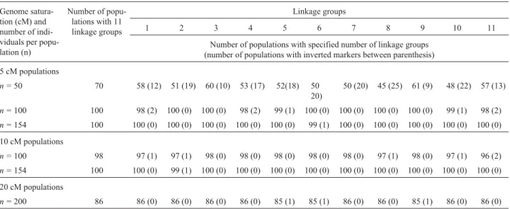
Table 2- Linkage groups with inverted markers. The table shows the genome marker saturation level (in cM) and the number of individuals (n) in each population size in respect to the number of populations with 11 linkage groups out of a total of 100 populations for each genome marker saturation level population size (n =50,n =100, etc). The number of populations (n =50,n =100, etc) with inverted markers (between parenthesis) was only evaluated in the populations that led the formation of 11 linkage groups.
Genome satura-tion (cM) and number of indi-viduals per popu-lation (n)
Number of popu-lations with 11 linkage groups
Linkage groups
1 2 3 4 5 6 7 8 9 10 11
Number of populations with specified number of linkage groups (number of populations with inverted markers between parenthesis)
5 cM populations
n =50 70 58 (12) 51 (19) 60 (10) 53 (17) 52(18) 50
20)
50 (20) 45 (25) 61 (9) 48 (22) 57 (13)
n =100 100 98 (2) 100 (0) 100 (0) 98 (2) 99 (1) 100 (0) 100 (0) 100 (0) 100 (0) 99 (1) 98 (2)
n =154 100 100 (0) 100 (0) 100 (0) 100 (0) 100 (0) 99 (1) 100 (0) 100 (0) 100 (0) 100 (0) 100 (0)
10 cM populations
n =100 98 97 (1) 97 (1) 98 (0) 98 (0) 98 (0) 98 (0) 98 (0) 97 (1) 98 (0) 97 (1) 96 (2)
n =154 100 100 (0) 99 (1) 100 (0) 100 (0) 100 (0) 100 (0) 100 (0) 100 (0) 100 (0) 100 (0) 100 (0)
20 cM populations
n =200 86 86 (0) 86 (0) 86 (0) 86 (0) 85 (1) 85 (1) 86 (0) 86 (0) 85 (1) 86 (0) 86 (0)
estimation of recombination frequency, as illustrated by the recombination frequency varianceVar r($) [= $r(1 2+ r$) /2 2n] (Schuster and Cruz, 2004) in whichnis the population size andr$is the maximum likelihood estimate of the recombina-tion frequency in the F2generation as function of the
ob-served recombination in the recombinant inbred lines,i.e.
$ / [ ( )]
r=R 2 1−R , where R is the recombination in the recombinant inbred lines (Burr and Burr, 1991). It is clear from this equation that a more accurate estimate of recom-bination frequency can be obtained either by increasing the population size or the level of marker saturation.
In the case of theLODscore as a factor influencing mapping, it is known that theLODscore is a function of sample size (n) and recombination frequency (R). TheLOD
score for recombinant inbred lines is given by
[
]
{
}
LOD= −R n+n R n+n −n
log10 0 5 1. ( ) 1 2( .0 5 )3 4( .0 25)
(Schuster and Cruz, 2004) in whichn1andn2are the
num-ber of individuals derived from non-recombinant gametes for a given pair of loci,n3andn4are the number of
individu-als derived from recombinant gametes for a given pair of loci andRis the recombination frequency in recombinant inbred lines. By replacing the values for population size and recombination frequencies in the expression above and consideringn1= n2= 0.5n(1-R)andn3= n4= 0.5nRit
fol-lows that whenRis fixed theLODscore values increase withn, e.g.if the recombination frequency in the corre-sponding F2(r) equals 0.05 for a 5 cM genome then for a
population size ofn =50 theLODscore is 8.43 while for
n =800 it is 134.98. Furthermore, whennis fixed a smallr
value results in a largeLODscore,i.e.for then =50 popu-lation theLODscore was 8.43 forr= 0.05, 5.26 forr= 0.1 and 2.06 forr= 0.20. Thus, the larger the number of indi-viduals genotyped for mapping, the larger theLODscore minimum value used to infer about linkage between mark-ers, providing more reliable linkage maps.
TheLODscore is limited to 2.06 for a population of
n =50 withr= 0.20, so if a minimumLODscore is selected which is greater than the value imposed by the size of the population then markers that should be linked will be in-ferred to be unlinked and the number of linkage groups will be increased. For all population sizes our evaluation used a minimumLODscore of 3 to infer linkage between markers, and since this value was greater than the 2.06 limitingLOD
score for a population size ofn =50 for a 20 cM genome this explains why some markers that should be linked were declared as unlinked for this population and genome satura-tion. TheLODscore is limited to 8.43 for a 5 cM genome with a population size ofn =50 but in our study the mini-mumLODscore of 3 was smaller than theLODscore
im-ulation sizes ofn= 50 andn= 100, theLODscores were greater than the threshold of 3, LOD = 5.26 and
LOD= 10.53, respectively.
By increasing population size or using populations with high linkage information it is possible to increase the probability for coupling genome segments as well as to in-crease genome coverage (Liu, 1998). In our study, consid-ering that the original genome saturation levels of 5 and 10 cM were satisfactory, a low number of recombinants in small populations might be an explanation for the establish-ment of a higher number of linkage groups than expected. We observed changes in the order of markers within link-age groups not only in the 5 cM genomen =50,n =100 and
n =154 populations but also in the 10 cM genomen =100 andn =154 populations and in the 20 cM genomen =200 population. Since these changes were more frequent in small populations the use of such populations can result in serious problems related to marker positioning in linkage groups and consequently generate false results in QTL mapping. The inversion of markers observed in this study has also been described by Liu (1998) as a function of pop-ulation size and map saturation level.
It is known that a better sampling of gametes is achieved as population size increases, leading to a better es-timate of recombination frequency. In our study, the size of linkage groups as well as the between-marker distances be-came closer to the true value of the simulated genome as population size was increased. Reduction in the variation (i.e.the standard deviation) of linkage group sizes between replications as population size increased indicated that better estimates of recombination frequency were achieved using large populations. It is possible to compare different genome saturation levels for a given population size using the mean deviation (d). For example, the percentage stress andd values for then =200 population were 25.1% and
d= 1.25 cM for the 5 cM genome population, 19.24% and
d= 1.92 cM for the 10 cM genome population and 15.02% andd= 3 cM for the 20 cM genome population, the stress values being shown in the last column of Table 1. Thus, al-though the percentage stress value was larger for the more marker-saturated genome the mean deviation value was smaller. Within the same genome saturation level the stress values decreased as population size increased, e.g. the stress anddvalues were 49.82% and 2.49 cM for then =50 population but 12.71% and 0.63 cM for then =800 popula-tion. Depending on the objectives of a particular study the determination of the population size and number of mark-ers to be used for mapping could be achieved by analyzing the magnitude of the mean deviation.
in genome mapping. However, high levels of accuracy are needed for QTL location when it is to serve as a basis for positional gene cloning (Van Ooijen, 1992; Liu, 1998). In this case, highly accurate QTL location estimates with a resolution of between 1 and 2 cM are needed for the appli-cation of physical mapping and QTL cloning procedures (Darvasiet al., 1993) and thus fine mapping techniques are necessary for obtaining better resolution. For plant breed-ing, however, high accuracy of distance estimates might not be so restrictive, since processes based on marker-assisted selection can be successful if the information about markers flanking a given QLT is available and the effect of the QLT can be easily detected (Van Ooijen, 1992).
A recombinant inbred line is an suitable population for estimating recombination frequency, especially when distances between markers are relatively short. On the other hand, gene linkage above 20 cM is not frequently de-tected in recombinant inbred lines because of the high re-combination frequency in this type of population, as already described by Burret al.(1988) and confirmed in our study.
Questions concerning the size of a recombinant in-bred line population and the number of markers needed to represent chromosomes in linkage groups have been ad-dressed previously (Ferreiraet al., 2006) but not with such an extensive genome as used by us. It is widely accepted that population size and the number of markers used in a study are frequently defined based on the availability of funds and genetic material. The application of our results will allow breeders to define the population size and the number of markers needed for the mapping of recombinant inbred lines. By analyzing 2100 maps obtained from simu-lated populations we concluded that: population size and number of markers are essential factors to be considered for obtaining reliable maps; maps with severe distortions were obtained with the use of small populations even using large number of markers; maps with severe distortions were ob-tained with the use of a small number of markers even using large populations; the minimum population sizes necessary for obtaining maps with the same number of markers per linkage group of simulated genomes weren =100 for the 5 cM population, n = 154 for the 10 cM population and
n =500 for the 20 cM population. Thus by increasing the saturation levels it is possible to substantially reduce the number of individuals to be genotyped. Alternatively, by genotyping a large number of individuals it is possible to reduce number of markers and still achieve a reliable map. Reasonable sizes of recombinant inbred lines necessary for obtaining reliable maps aren =200 for a genome saturation level of 5 cM,n = 300 for a genome saturation level of 10 cM andn =500 for a genome saturation level of 20 cM.
Acknowledgments
The authors wish to thank the Brazilian agencies CAPES, CNPq and FAPEMIG for financial support and the
anonymous reviewers for their invaluable suggestions for improving this manuscript.
References
Burnham KD, Dorrance AE, Vantoai TT and Martin SKSt (2003) Quantitative trait loci for partial resistance toPhytophtora sojaein soybean. Crop Sci 43:1610-1617.
Burr B and Burr F (1991) Recombinant inbreds for molecular mapping in maize: Theoretical and practical considerations. Trends Genet 7:55-60.
Burr B, Burr FA, Thompson KH, Albertson M and Stuber CW (1988) Gene mapping with recombinant inbreds in maize. Genetics 118:519-526.
Cardinal AJ, Lee M, Sharopora N, Woodman-Clikeman WL and Long MJ (2001) Genetic mapping and analysis of quantita-tive trait loci for resistance to stalk tunneling by the Euro-pean corn bores in maize. Crop Sci 41:835-845.
Darvasi A, Weinreb A, Minke V, Weller JI and Soller M (1993) Detecting marker-QTL linkage and estimating QTL gene ef-fect and map location using a saturated genetic map. Genet-ics 134:943-951.
Deorge R (1993) Constructing genetics maps by rapid chain delin-eation. J Quant Trait Loci 2:121-132.
Faleiro FG, Ragagnin VA, Schuster I, Corrêa RX, Good-God PI, Brommonshenkel SH, Moreira MA and Barros EG (2003) Mapeamento de genes de resistência do feijoeiro à ferrugem, antracnose e mancha-angular usando marcadores RAPD. Fitopatol Bras 28:59-66.
Falk CT (1989) A simple scheme for preliminary ordering of mul-tiple loci: Application to 45 CF families. In: Elston, Spence, Hodge and Cluer (eds) Multipoint Mapping and Linkage Based Upon Affected Pedigree Members (Genetic Work-shop 6). Liss, New York, pp 17-22.
Ferreira A, da Silva MF, Silva LC and Cruz CD (2006) Estimating the effects of population size and type on the accuracy of ge-netic maps. Genet Mol Biol 29:187-192.
Ferreira AR, Foutz KR and Keim P (2000) Soybean genetic map of RAPD markers assigned to an existing scaffold RFLP map. Am Genet Assoc 91:392-396.
Kruskal JB (1964) Multidimensional scaling by optimizing good-ness of fit to a non-metric hypothesis. Psychometrika 29:1-27.
Lander ES and Botstein D (1989) Mapping Mendelian factors un-derlying quantitative traits using RFLP linkage maps. Ge-netics 121:185-199.
Liu BH (1998) Statistical genomics, linkage, mapping and QTL analysis. CRC Press, Boca Raton, 854 pp.
Miklas PN, Johnson WC, Delorme R and Gepts P (2001) QTL conditioning physiological resistance and avoidance to white mold in dry bean. Crop Sci 41:309-315.
Schuster I and Cruz CD (2004) Estatística Genômica Aplicada a Populações Derivadas de Cruzamentos. Editora da Universidade Federal de Viçosa, Viçosa, 568 pp.
Van Ooijen JW (1992) Accuracy of mapping quantitative trait loci in autogamous species. Theor Appl Genet 84:803-811. Xing YZ, Tan YF, Hua JP, Sun XL and Xu CG (2002)
Character-ization of the main effects, epistatic effects and their envi-ronmental interactions of QTLs on the genetic basis of yield traits in rice. Theor Appl Genet 105:248-257.