Ricardo Biloti,
1Lúcio T. Santos,
2Martin Tygel
3 Submetido em 15, agosto, 2003/Aceito em 31, março, 2004Submited August 1, 2003/Accepted March 31, 2004
ABSTRACT
We propose a method that is capable to filter out noise as well as suppress outliers of sampled real functions under fairly general conditions. From an a priori selection of the number of knots that define the adjusting spline, but not their location in that curve, the method automatically determines the adjusting cubic spline in a least-squares optimal sense. The method is fast and easily allows for selection of various possible number of knots, adding a desirable flexibility to the procedure. As an illustration, we apply the method to some typical situations found in geophysical problems.
Keywords: Smoothing, cubic splines RESUMO
Propomos um método capaz de filtrar ruído bem como suprimir outliers de uma função real amostrada, impondo praticamente nenhuma condição. A partir de uma seleção a priori da quantidade de nós que definirão a spline, porém não suas localizações, o método automaticamente determina a spline cúbica que melhor ajusta os dados, no sentido de quadrados mínimos. Dado que o método é rápido, torna-se viável a realização de vários ajustes com quantidades distintas de nós, conferindo assim a flexibilidade desejada ao processo. Como exemplo, aplicamos o método a alguns problemas em Geofísica.
Palavras-chave: suavização, spline cúbica
1 Universidade Federal do Paraná - Departamento de Matemática Centro Politécnico, Jd. das Américas - Cx.P. 19081 - CEP 81531-980, Curitiba, PR - Fone/fax: (41) 361 3400 - e-mail: [email protected]
interpolation approach, where the noisy data is replaced by corresponding points that belong to an interpolating function.
The natural question is how should we choose the “interpolating points” from the data so as to construct the desired smoothing function. Normally, these points are extracted from the data, in a regular fashion or manually selected.
We propose a method that optimally selects points to define a cubic spline that best represents the data in the least-squares sense. An interesting feature of the method is that the knot points are no longer required to belong to the original data set. As we will see below, the method is suitable, not only for smoothing, but also for discarding outliers. The method is designed to handle datasets composed by samples of rather complicated real functions. It is to be stressed that, by construction, the obtained function is naturally smooth up to second-order derivative. The proposed method is applied to two important problems in geophysics. The first problem is to recover horizons as part of a macro-velocity model inversion from multi-coverage seismic data and to smooth seismic traveltime attributes (BILOTI; SANTOS, 2002). The second application refers to smoothing well-log data for anomaly detection and inversion purposes.
FORMULATION
Consider a noisy data Ω =
{
(
x yj, j)
∈IR |j= ,...,M}
2
1
be the number of interpolating points and Γ =
{
(
X Yi, i)
∈IR | 2< =
}
−
Xi X ii N
| 1 , 1,..., be the set of these points that defines the
sought-for cubic spline. To obtain the best set Γ, in the least-squares sense, we must solve the 2N-variable problem
minΓ |yj s x , j M j =
∑
−( )
1 2 s.t.s is the cubic spline defined by ΓΓ
X1 ≥ ≤ min max j x j XN j xj . (1)
given set Ω, that is, (Xi, Yi)=(xj,yj), with j= + −1
( )
i 1 . .(M–1)/(N −1) , for i=1,...,N, where
x
denotes the greater integer less than or equal to x.Note that we have not made any consideration on how to choose the number, N of interpolating points. The method is designed to automatically find, in the least-squares sense, the best cubic spline for the specified number of knots N. Of course, for a small number of points N, the obtained spline will not be able to represent more than the general trend of the curve. On the other extreme, for large values of N, the spline will tend to fit even the outliers. Since the method is fast, it is reasonable to estimate the cubic spline for several choices of N. This flexibility can be very useful to the user or interpreter, in the sense that a number of inexpensive trials can be implemented before a final decision on which level of smoothness is the best choice for the problem.
APPLICATIONS
We now illustrate the application of the proposed method to some common practical situations. We start by testing the ability of the method to smooth a sequence of the four datasets of increasing difficulty, shown in Figure 1. We next apply the procedure to two problems related to seismic imaging and inversion, shown if Figures 2 and 3, respectively.
General Situations
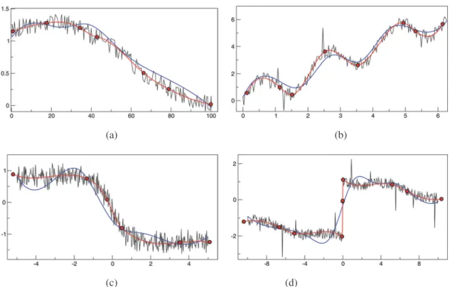
Figure 1(a) shows that the method efficiently handles and removes white noise. In the next example (Figure 1(b)), besides the noise, some outliers were added. Again, the optimized cubic spline represents the data very well. In Figure 1(c), we see that the obtained curve is able to well describe abrupt variations of the data. Finally, in Figure 1(d), we see that the method is robust enough to provide good results even in the presence of discontinuities. Note that, in particular, there are no Runge effects near the discontinuities.
(a) (b)
(c) (d)
Figure 1 – Examples of cubic spline optimal adjust. In all graphs the black line represents the noisy data (linearly interpolated), the blue line states for the initial approximation for the optimization solver, the red line is the optimized cubic spline obtained, and the red dots are the knots that define that spline.
Figura 1 – Exemplos do ajuste ótimo de splines cúbicas. Em todos os gráficos, a curva em preto representa o dado com ruído
(interpolado linearmente), a curva azul representa a aproximação inicial para o otimizador, a curva vermelha é a spline cúbica ótima obtida e os círculos vermelhos são os nós que definem a spline.
HORIZON RECONSTRUCTION
We present the results of an algorithm for reconstruction of interfaces and inversion of attributes from 2D-multi-coverage seismic data. As reported in Biloti et al. (2001), the procedure has been successfully applied to invert a layered macro-velocity model from the data. Figure 2(a) depicts the inverted model, where the estimated interfaces (solid lines) were approximated by conventional cubic splines (constructed by selection of knots among the sampled set). In Figure 2(b), we can see the improvement of the inverted model, when the interfaces where constructed upon the application of the proposed technique.
WELL-LOG ANALYSIS
Well logs play the important role of linking rock parameters to
anomalies. Well data (e.g., P-and S-velocities and density) are, in general, very noisy, so it may be desirable to consider the parameters as smooth functions of depth (or time). Figure 3 shows the application of the method to smooth a couple real data well logs. On the top of the figure, the new method was used with N = 20 knots. On the bottom of the figure, the number of knots was N = 30.
CONCLUSIONS
We presented an automatic method for smoothing and outlier suppression of data sets that consist of sampled real function points. After an a priori selection of the number of knots, the procedure automatically finds the location of the interpolating points, in such a way that the resulting smoothing function (a cubic spline) is optimal in the least-squares sense. As the method is fast, it allows the user to apply the procedure to different numbers of knots, so as to choose the degree
Figure 2 – Multiparametric traveltime attributes inversion. The dashed lines represent the real interfaces and the solid lines represent the obtained ones. In (a) the interfaces were approximated by interpolating splines, and in (b) they were approximated by optimal splines.
The real and the estimated velocities are vi and e i
v , respectively.
Figura 2 – Inversão de atributos de tempo de trânsito multiparamétrico. As linhas tracejadas representam as interfaces reais e as linhas sólidas representam as interfaces obtidas. Em (a) as interfaces foram aproximadas por splines interpolantes, e em (b) elas foram aproximadas por splines ótimas. As velocidades reais e estimadas são vi e e
i
v , respectivamente.
optimization method with spectral projected gradients. Computational Optimization and Applications, [S.l.], v. 23, p. 101-125, 2002.
(b)