Pedro Filipe Guerreiro Canelas

Março, 2016

Pedro Filipe Guerreiro Canelas

Licenciado em Ciências da Engenharia Biomédica

Simulation of biologically inspired object movement

for the study of object tracking algorithms

Dissertação para obtenção do Grau de Mestre em Engenharia Biomédica

Orientador: José Manuel Fonseca, Professor Auxiliar, Faculdade de Ciências e Tecnologias da Universidade Nova de Lisboa

iii

Simulation of biologically inspired object movement for the study of object tracking algorithms

Copyright © Pedro Filipe Guerreiro Canelas, Faculdade de Ciências e Tecnologia, Universidade Nova de Lisboa.

v

“All we ever see of stars are their old photographs.”

vii

Acknowledgments

I want to thank my supervisor Prof. Dr. José Manuel Fonseca for all the help, guidance and motivation that helped me finish this work, for his useful critiques and for his persistence.

Thank you to all CA3 team, especially to Leonardo Martins, that was a very important help in the development of this dissertation, writing of the paper, and was a great help in keeping my schedules.

Thank you to all my friends from this course, specially in this last year, the most challenging and interesting one, and for all ideas changed with them.

ix

Abstract

Major advances in Cell and Molecular Biology have been associated with the advances in live-cell microscopy imaging, and these studies started to rely on temporal single cell imaging. To support these efforts, available automated image analysis methods such as cell segmentation and cell tracking during a time-series analysis should be improved. One important step is the validation of such image processing methods. Ideally, the “ground truth” should be known, which is possible only by manually labelling images or by artificially produced images. To simulate such artificial images we developed a platform that can simulate biologically inspired objects, by generating bodies with different morphologies, physical movement and that can aggregate in clusters. Using this platform, we tested and compared four tracking algorithms: Simple Nearest-Neighbour (NN), NN with Morphology and two DBSCAN based ones. In this work we showed that Simple NN work for small object velocities, while the other algorithms perform better on higher velocities and when clustered. This platform can generate new benchmark images and is openly available to test other tracking algorithms. (http://griduni.uninova.pt/Clustergen/ClusterGen_v1.0.zip)

xi

Resumo

Os maiores progressos na Biologia Celular e Molecular têm estado associados aos progressos nas imagens microscópicas de células, e os estudos desse género já começaram a ter em conta imagens temporais. De forma a melhorar resultados, os métodos automáticos de análise de imagem, como a segmentação e seguimento de células deverão ser aperfeiçoados. Um dos pontos mais importantes é a validação desses métodos de processamento de imagem, o que é unicamente possível através da identificação manual das imagens ou por imagens produzidas artificialmente. De forma a simular esse tipo de imagens artificiais, foi criada uma plataforma com a capacidade de simular objetos de inspiração biológica, gerando corpos com diferentes morfologias, movimento físico e que se podem agrupar em clusters. Esta plataforma foi utilizada para testar e comparar quatro algoritmos de seguimento: Nearest Neighbour simples (NN), NN com Morfologia e dois algoritmos baseados no algoritmo DBSCAN. Com este trabalho mostrou-se que o NN simples pode ser utilizado para objetos a baixa velocidade, enquanto os restantes algoritmos trazem melhores resultados para maiores velocidades e para objetos agrupados em clusters. A plataforma criada pode gerar novas imagens de referência e está disponível (http://griduni.uninova.pt/Clustergen/ClusterGen_v1.0.zip) para testes a outros algoritmos de teste.

xiii

Content

Introduction ... 1

State of The Art ... 3

2.1 Image Generator ... 3

2.2 Tracking Methods ... 7

Methodologies ... 15

3.1 Image Generator ... 15

3.1.1 Interface ... 16

3.1.2 Object Motility ... 18

3.1.3 Clustering ... 19

3.1.4 Divisions ... 21

3.2 Tracking Methods ... 22

3.2.1 Simple Nearest Neighbour Algorithm ... 22

3.2.1 Nearest Neighbour with Morphology Algorithm ... 22

3.2.2 Cluster Tracking ... 25

3.2.2.1 Cluster Identification ... 25

3.2.2.2 Tracking ... 26

Results and Discussion ... 31

4.1 Simple Nearest Neighbour Algorithm ... 31

4.2 Nearest Neighbour with Morphology Algorithm ... 32

xiv

4.3.1 Simple Nearest Neighbour and Nearest Neighbour with Morphology 39 4.3.2 DBSCAN Related Tracking ... 42

Conclusions and Future Work ... 45

xv

List of Figures

Figure 2.1: Example of an image created by ‘SIMCEP’ ... 4

Figure 2.2: Example of images created by ‘CytoPacq’. ... 5

Figure 2.3: Example of an image created by ‘SimuCell’.. ... 6

Figure 2.4: Example on an image created by ‘CellOrganizer’. ... 6

Figure 2.5: Different object representations. ... 8

Figure 2.6: Organization of tracking methods. ... 9

Figure 3.1: Main Interface of Time-Series Generator ... 16

Figure 3.2: Main Interface left bar ... 17

Figure 3.3: Pop-up with properties for cluster creation ... 18

Figure 3.4: Collision between objects with "Physical Move". ... 19

Figure 3.5: Example of "Follow the Leader" Movement ... 20

Figure 3.6: Example of “Alternative Movement” ... 21

Figure 3.7: Example of object division ... 22

Figure 3.8: Flow Chart of Nearest Neighbour Algorithms ... 24

Figure 3.9: Example of a possible misidentification using Nearest NeighbourNN Algorithms ... 25

Figure 3.10: Representation of object identification in clusters ... 26

Figure 3.11: Flow chart of first process of DBSCAN based tracking algorithm ... 27

Figure 3.12: Flow chart of second process of DBSCAN related tracking algorithm ... 29

Figure 4.1: Simple Nearest Neighbour results with different maximum velocities. ... 32

Figure 4.2: Nearest Neighbour with Morphology results for Test 1 with mmd=0.05. ... 33

Figure 4.3: Nearest Neighbour with Morphology results for Test 2 with mmd=0.05. ... 35

Figure 4.4: Nearest Neighbour with Morphology results for Test 1 with mmd=0.10. ... 36

xvii

List of Tables

xix

Acronyms and Symbols

NN NNm DBSCAN CCD RNA PDAF MHT JPDAF KLT SIFT ROI CSV Eps MinPts mmd Nearest Neighbour

Nearest Neighbour with Morphology

Density-based spatial clustering of applications with noise

Charge-Couple Device

Ribonucleic Acid

Probabilistic Data Association Filter

Multiple Hypothesis Tracking

Joint Probabilistic Data Association Filter

Kenade-Lucas-Tomasi

Scale Invariant Feature Transform

Region of Interest

Comma Separated Values

Neighbourhood Radius

Minimum Points

1

Introduction

Some of the major discoveries in Cell and Molecular Biology have been associated with the advances in live-cell microscopy imaging, contributing to the acquisition of images with better quality and resolution and in techniques capable of detecting and observing newly discovered cellular dynamics and structures [1], [2].

The fundamental challenges in live-cell imaging can be divided into two major areas. The first area is related to the processes that occur previous and during the image acquisition in the laboratory, associated with the refinement of the automatic acquisition processes (illumination, focus, drift correction, stage positioning, etc) and the improvement of the microscope components (e.g. shutter, lens, camera, stage) [3]. The second area is related to the post processing limitations, associated with storage and archiving of a large amount of data and the image analysis processes (background correction, registration of multimodal and multidimensional images, segmentation, tracking, statistical quantification and modelling of the object’s behaviour) [3], [4].

Automatic correction algorithms are normally included in microscope software packages [5], while the process of image registration (overlaying two or more images of the same location taken at different time frames and/or from different viewpoints and/or by different sensorial devices) has been extensively studied can be classified based on the modality, intensity, the type of data, dimensionality, the domain and type of transformation and the registration methodologies [6], [7].

The post-process analysis of the image time-series is usually made in three steps: segmentation, tracking, and recognition of the object’s behaviour. In the first

2

step, the objects being tracked are detected, located, and separated from the background.

Segmentation is out of the scope of this work, which means that the objects from the time-series are supposed to be already segmented and with the information required to perform the tracking.

Object tracking in general is becoming an important subject, with applications in vehicle and people tracking, medical diagnosis, surveillance, body motion analysis, among others [1].

The goal of this work is to test several tracking algorithms in different situations, like objects moving freely or grouped in clusters. In order to have standard images to test these algorithms, a Time-Series Generator platform was developed. This Generator allows the creation of different types of object movement and characteristics arbitrarily created, with control over several parameters.

3

2.

State of The Art

2.1

Image Generator

In order to prevent the abusive comparison of image processing techniques, there have been contests and open challenges organized, requiring that every methodology is tested on the same benchmark data-sets (acquired by an independent laboratory or created by artificial image generators) [8]. Such artificial image generators require realistic biological models to be relevant in such biological studies. These tools, normally use data coming from theoretical and experimental information obtained from statistical distributions of the object’s behaviour [9] but also spatial and temporal data from the objects [10], [11]. If the studied object is a cell, these models should include morphology parameters such as cell shape and size, location of subcellular structures, kinetic and spatial statistics of cell growth, cell division, cell migration and models of internal cell functions. Focusing on the available tools that simulate microscopy images based on biological models, these can be divided in three main phases: the digital phantom object generation, the simulation of the signal passing through the optical system and the simulation of the image formed on a specific sensor [12].

Simulators such as ‘SIMCEP’ [13] have provided a gold-standard platform to validate and test various image processing tools, such as ‘CellC’ [14], the open-source and Java-based image processor: ImageJ and the commercially available software: MCID Analysis (Imaging Research Inc., Catharines, ON, Canada; Evaluation ver. 7.0), along with other image processing tools [15]. The phantom objects generated with different cell parameters, such as probability of clustering, cell radius, and cell shape and with parameters related to the sensors and the optical system such as background

4

noise and illumination disturbance [15], [16]. ‘SIMCEP’ has the ability to create either a population with similar characteristics, or sub-populations with their own characteristics [13], and an example can be seen in Figure 2.1. Generation of objects is done sequentially, starting with a simple ellipsoid in black and white and then transforming it, adding internal structures and the nucleus [17].

Another toolbox called ‘CytoPacq’ was developed specifically to simulate all three phases, by being equipped with three different modules. In Figure 2.2 there is an example of a result of this toolbox. The first module (‘3D-cytogen’) generates the digital object phantom, which imitates the cell structure and behaviour and has been shown to generate microspheres, granulocytes, HL-60 Nucleus and images of Colon Tissue. The second module (‘3D-optigen’) simulates the transmission of the signal through the lenses, objective, excitation filter and emission filter (various sets of equipment can be simulated). The last module, ‘3D-acquigen’ is the digital CCD camera simulator of the phenomenon’s that occur during image capture (noise, sampling, digitization) by changing the camera selection, the acquisition time, the dynamic range usage and the

5

stage z-step [12], [17]. The same group also introduced a novel versatile tool (‘TRAgen’) capable of generating 2D time-lapses by simulating living cell populations as a ground-truth for the evaluation of cell tracking algorithms. They also include models of cell motility, cell division and cell clustering up to tissue-level density [18]. Both these simulators have been an important step in the simulation of cellular dynamics, such as measuring protein or RNA levels or even observing cell migration, cell division and cell growth [2], [3].

A recently developed toolbox called ‘SimuCell’ [19] is capable of generating artificial microscopy images with heterogeneous cellular populations and diverse cell phenotypes. Each cell and their organelles are modelled with different shapes, having distinct distributions of biomarkers over each shape, which can be affected by the cell’s microenvironment, showing the importance of good cell placement (e.g. in clusters, overlapping existing cells) [19]. ‘SimuCell’ can also simulate image acquisition or cell artefacts, and an example of it is in Figure 2.3.

Figure 2.2: Example of images created by ‘CytoPacq’. Adapted from

6

The ‘CellOrganizer’ toolbox was developed using a different approach, collecting laboratory data and using machine-learning techniques to generate the entire cell,

Figure 2.43: Example of an image created by ‘SimuCell’. Adapted from [19].

Figure 2.34: Example on an image created by ‘CellOrganizer’. Adapted

7

including structures such as the nucleus, proteins, cell membrane and cytoplasm components [20]. Although the learn-based model was capable of extracting a very precise shape model, they couldn’t be described it in precise mathematical terms [21].

Most of these image generators have focused on the simulation of morphological features and spatial information of the cell. Morphological information can be enough to create multidimensional images, but cannot simulate time-lapsed multimodal and functional images, where important time-dependent processes are present. To simulate such images of bacterial cells, the ‘miSimBa’ (Microscopy Image Simulator of Bacterial Cells) tool has been under development [22]. The simulated images can reproduce spatial and temporal bacterial time-dependent processes by modelling, cell growth, division, motility and cell morphology (shape, size and spatial arrangement) [22].

These simulation tools can also be used to generate “null-models” [23] to study statistical patterns in absence of a particular mechanism (e.g. removing the nucleoid to study how it influences the production of RNA molecules).

2.2

Tracking Methods

8

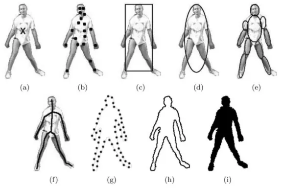
A lot of tracking methods have been proposed through the years, differing mainly in the approach they make to the available object features and the type/number of objects to work with. In order to decide which approach to follow, the object’s representation should be taken into account, and this is defined during segmentation. Objects can be represented through points, geometric shapes, silhouette and contour, articulated shape models, and skeletal model, as seen in Figure 2.5. These types of object’s representation lead to different tracking approaches.

Yilmaz et al. [24] made an extensive revising of the “generic” tracking methods and divides them in three main categories as seen in Figure 2.6.

Figure 2.5: Different object representations: (a) Centroid, (b) Multiple Points, (c) Rectangular Path, (d) Elliptical Path, (e) Part-based Multiple Patches, (f) Object Skeleton, (g) Control Points on Object Contour, (h) Complete Object Contour, (i) Object

9

In Point Tracking, objects are represented by points, which are associated, frame by frame, based on the object’s position and motion. Problems in tracking objects by point correspondence are the presence of occlusions, misdetections, entries and exits of objects. It can be split in Deterministic and Statistical methods. Deterministic methods associate each object with the application of motion constraints. Statistical methods use random perturbations and noise into account while making the correspondence [24].

Nearest Neighbour (NN) is the simplest method and the source of all deterministic approaches. This method uses only the distances between objects in k and k-1 and matches the ones with minimum distances [26]. The distance between objects can be based on the position, shape, colour, size, etc.

Gu et al. [27] proposed a method combining NN classification with SIFT descriptors, efficient subwindow search and an updating and pruning method to achieve balance between stability and plasticity, in order to handle appearance changes. This method led to efficient results, being able to handle occlusions, clutter, and changes in scale and appearance.

10

The probabilistic data association filter (PDAF) and the joint probabilistic data association filter (JPDAF) are the most basic statistical methods. PDAF uses a weighted average of the validated measurements as input, modelling only one target and considering linear dynamic and measurement models. JPDAF is an extension of PDAF, allowing multiple target tracking. The assumptions are the same, calculating the target’s association probabilities jointly. In both methods, the Kalman Filter is very important, if the model is linear. In JPDAF, linearization is only possible if the nonlinearities are weak in the ROI. One of the problems of these methods is the incapacity to recover from errors, because only the last measurement is used [26].

Gorji et al. [28] developed a combined method of JDPAF and a particle filtering [29], calling it Monte Carlo JPDAF. This method used three different models. One with near constant velocity, other with near constant acceleration and a third combining the other two. The combined method was the one with better performance on the tests made.

Other statistical method is the multiple hypothesis tracking (MHT). This method is one of the most used with point features, but is computationally exponential, both in time and memory [30]. This method postpones data association until enough information is available. The MHT starts by formulating all possible hypotheses, which develop to a set of new hypotheses each time new data arrives, generating a tree of hypothesis [26]. For each hypothesis, the position of the object in the next frame is predicted, and then compared with the measurements, calculating their distance. The associations are made for each hypothesis, generating new hypotheses for the next iteration [24]. The tree of hypothesis should be cut, because it grows exponentially with the measured data. This can be done by clustering, which means that measurements are subdivided into independent clusters. If a measurement can not be associated with an existent cluster, a new one is created. Other way of cutting the tree is pruning, which means that as new iterations come, a part of the tree is deleted [26]. Unlike PDAF and JPDAF, MHT can deal with objects entry, exit and occlusion.

Kernel Tracking can be done using templates and density-based appearance models, or multiview appearance models. Templates use basic geometric shapes, while multiview models encode different views of the object [24].

11

Bhattacharyya coefficient [31] and the Kullback-Leibler divergence [32]. The process has several iterations, in a way to increase similarity between histograms, repeated until they converge [33]. KLT is an optical-flow method, which uses vectors to show the changes in the image (i.e. translation). Shi and Tomasi proposed a version of this method, in which the translation of a region centered on an interest point is iteratively computed. Then, the tracker evaluates the quality of the tracked patch, computing a transformation between the corresponding patches in consecutive frames [34]. These methods are effective while tracking single objects, but have problems with multiple objects.

Silhouette Tracking consists in using precise information about the shape of the objects. Tracking can be done by Shape Matching, which searches an object silhouette and its model in each frame, and each translation from frame to frame is handled separately, or by finding corresponding silhouettes detected in two consecutive frames. Contour tracking is also an approach, and it’s based in the evolution of the contour of an object, connecting the correspondent objects by state space models or by minimizing the contour energy [24].

When tracking objects, we usually obtain multiple measurements, and the incorrect ones are referred to as false measurements or clutter. Data association is, then, selecting the measurement that has the highest probability of being originated from the object to be tracked. If the algorithm selects the wrong measurement or the correct measurement isn’t even detected, can result in poor state estimates. To solve this problem, we select a validation region, called measurement gate. The measurement gate is a region in which the next measurement has a high probability to appear, also reducing computational cost [26].

The Kalman filter is an optimal estimator, which means that it assumes parameters from indirect, inaccurate and uncertain observations, and if all noise is Gaussian, the linear Kalman filter minimizes the mean square error of the estimated parameters [26]. This filter is widely used to obtain the optimal state estimate in several approaches.

12

𝑥𝑘+1 = 𝐹𝑘𝑥𝑘+ 𝐺𝑘𝑢𝑘+ 𝑣𝑘 _(2.1)

𝑧𝑘 = 𝐻𝑘𝑥𝑘+ 𝑤𝑘 _(2.2)

Where Fk and Hk are the transition and the observation model, and uk is the dimensional known input vector. To estimate the state we must know 𝑥̂_𝑘|𝑘, uk, zk+1, and

Pk|k (the covariance of xk). The time update phase lies in the state prediction:

𝑥̂𝑘+1|𝑘 = 𝐹𝑘𝑥̂𝑘|𝑘 + Gkuk _(2.3)

And in the measurement prediction:

𝑧̂𝑘+1|𝑘 = 𝐻𝑘𝑥̂𝑘+1|𝑘 _(2.4)

The measurement update phase lies in the measurement residual:

𝑣𝑘+1 = 𝑧𝑘+1− 𝑧̂𝑘+1|𝑘 _(2.5)

And in the update state estimate:

𝑥̂𝑘+1|𝑘+1= 𝑥̂𝑘+1|𝑘+ 𝐾𝑘+1𝑣𝑘+1 _(2.6)

In which Kk+1 is the Kalman Gain. The state covariance should be estimated too. So, the state prediction covariance is:

𝑃𝑘+1|𝑘 = 𝐹𝑘𝑃𝑘|𝑘𝐹𝑘′ + 𝑄𝑘 _(2.7)

The measurement prediction covariance is:

𝑆𝑘+1= 𝐻𝑘+1𝑃𝑘+1|𝑘𝐻𝑘+1′ + 𝑅𝑘+1 _(2.8)

Then, the Kalman Filter Gain is:

13 And the updated state covariance:

𝑃𝑘+1|𝑘+1= 𝑃𝑘+1|𝑘− 𝐾𝑘+1𝑆𝑘+1𝐾𝑘+1′ _(2.10)

15

3.

Methodologies

3.1 Image Generator

The image generator interface and the tracking methods were implemented using the C# language from the Visual Studio 2015. An intuitive and easy to understand interface was designed in order to facilitate the analysis of the tested tracking algorithms. The time-series generator allows the user to change a set of settings such as the number of objects, frames and clusters, and their features.

The generator creates two csv files for each of the object’s properties (position in x and y coordinates and a shape-related factor called “morphology”, which is a rational number between 0 and 1), where in the first one values are not organized by objects, and the second file is called “tracked”, which each column of the csv file corresponds to one object.

In this generator, objects are represented by circles and the morphology factor is assumed as the radius. There is a conversion factor that determines the maximum radius of the objects (corresponding to morphology value 1), and this factor is initialized at 30. More factors and parameters can be added to the algorithm, increasing its complexity.

16

3.1.1 Interface

The user’s interface is intuitive and easy to understand, and is shown in Figure 3.1. At the top row of the window are the frame handlers, allowing to go forward and backward in the time-series, or to go directly a specific frame. The “Time-Lapse” button reproduces the full time-series in one time, one frame per each 40 milliseconds.

Figure 3.1: Main Interface of Time-Series Generator

17

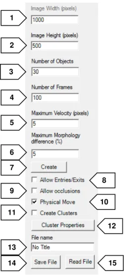
If “Allow Entries/Exits” (8) is selected, objects can enter and exit the image limits. If not, they collide with the edges when close to them, with their move depending on whether or not they have physical move. This process is explained in Section 3.1.2.

If “Allow Occlusions” (9) is selected, objects can move with no restrictions due to superposition between them, allowing overlapping. If not, objects collide between them in a similar way as when they collide with the edges.

“Physical Move” (10) button controls the option of giving objects physical limitations to their move. If it is selected, objects will have velocity and orientation assigned to each of them, meaning that their position variance will depend on these two variables. If it is not, objects will move arbitrarily through the image.

The “Create Clusters” (11) checkbox is used to organize objects into clusters, giving objects of the same cluster the same physical features. If it is selected, “Physical

Figure 3.2: Main Interface left bar

18

Move” is automatically selected and “Allow Occlusions” deselected, blocking their checkboxes.

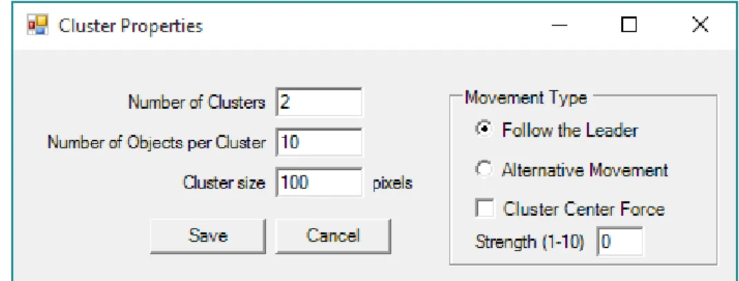
The button “Cluster Properties” (12) leads to a new window with the options for clusters’ creation represented in Figure 3.3. It is possible to choose the desired number of clusters, the number of objects per cluster, and the size of the clusters, in pixels. It is also possible to choose between two movement types of objects’ movement through the frames, “Follow the Leader” and “Alternative Movement”, as the application of a “Cluster Centre Force”, and its strength. The application of these parameters is explained in Section 3.1.3.

“File name” (13) allows the user to choose the name to give to the files when saving them, “Save File” (14) saves the csv files in the designated folder, and “Read File” (15) opens a previous generated and saved Time-Series.

3.1.2 Object Motility

According to user’s selection, objects can have movement respecting some physical rules. If this option is deactivated, objects will move arbitrarily through the image. Objects in each frame are only represented by their position in coordinates x and y, as their morphology factor, meaning that their position variance is random. In each frame, each object has a new x and y coordinates distanced an arbitrary distance from the coordinates in previous frame, not more than the value at “Maximum Velocity”, in pixels. With occlusions and exits and entries also deactivated, objects will just avoid the positions where they collide with other objects or go out the image boundaries, searching for a position considering these limitations and the maximum distance they can go.

19

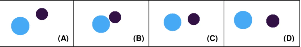
If the user chooses to give objects “Physical Move”, in addition to previous features, each object will have also velocity and orientation (physical parameters) assigned to each of them, meaning that their position variance will depend on this two variables. In each frame, each object will have new x and y coordinates distanced “d” from the coordinates in previous frame, in direction “o”, being “d” the velocity assigned to it, no bigger than “Maximum Velocity”, and “o” the orientation, between 0 and 2pi radians, both of them with an independent and small arbitrary component. If entries and exits are deactivated, if an object is heading to the image boundary it is reflected respecting Snell’s Law, causing a change in its orientation. If occlusions are deactivated, if two objects are going to collide, they change their orientation to opposite directions to each other, in an approximation to the reflection laws, but ignoring their differences in morphology.

In Figure 3.4 there is an example of a collision between two objects with Physical move in 4 frames of a Time-Series.

3.1.3 Clustering

When selecting option “Create Clusters”, the Generator will create a time-series with the number of clusters, objects and size of cluster chosen by the user. These options should be consistent and take into consideration the image size.

In “Follow the Leader” movement type, each cluster has a leading object, which means that characteristics of the other objects of the same cluster are dependent on the leader behaviour. The leader “receives” the physical parameters at first frame (velocity and orientation) and at each frame the other objects of its cluster will move in the leader’s direction, minimizing the distance from it, respecting the “non-collision” rule. If two objects from different clusters collide, one of them will start belonging to the other cluster. This may cause the “merging” of clusters. This type of movement is represented in Figure 3.5.

(A) (B) (C) (D)

20

In “Alternative Movement”, all objects of each cluster have the same physical parameters, which means that they move in the same direction with the same velocity (with a little independent arbitrary component). “Cluster Centre Force” is a feature exclusively for “Alternative Movement” and creates an attraction force at the cluster’s centre, with a selectable strength selected by the user. This force keeps cluster’s objects hold together, even when colliding with image limits or other objects. As higher the strength, quicker the objects move to the cluster’s centre. In this movement type, when objects from different clusters collide, they will be “left behind” by their cluster until they can join it again. This type of movement is illustrated in Figure 3.6.

21

3.1.4 Divisions

The last feature added to this generator was object division. This feature is intended to be an approximation to living cell proliferation, where a parent cell “splits” in half, originating two daughter cells. In this specific case, since objects are represented only by circles, and not by complex shapes, division consists in splitting an object with morphology factor m in two objects with factor m/2.

There was a factor named “Division Probability”, measured in percentile that defines the probability of occurring a division for each object, in each frame of the time-series, being an arbitrary happening. Daughter objects inherit from parent the physical parameters and belonging cluster. In Figure 3.7 it is shown an example of a division.

22

3.2

Tracking Methods

3.2.1 Simple Nearest Neighbour Algorithm

The first algorithm to be tested is the Simple Nearest Neighbour (NN). This method only takes in consideration the physical positions of each objects in each frame of the time-series, and uses the Euclidian Distance between points to find matching

objects between frame n and n+1. Being

𝑑

𝑑𝑝= √(𝑥𝑛− 𝑥𝑛+1)2+ (𝑦𝑛− 𝑦𝑛+1)2 (3.1)

Where 𝑥_𝑛 and 𝑦_𝑛are the positions of each object in frame n and 𝑥_𝑛+1and

𝑦𝑛+1 are the positions in frame n+1. Having the distance between each object in frame

n and all objects in frame n+1, correspondences are made based on the minimum distance. The object in frame n+1 closer to each object in frame n are assigned to it. If two objects in n+1 are assigned to the same object in n, the closer object is assigned, until all correspondences between frames are unique.

3.2.1 Nearest Neighbour with Morphology Algorithm

The next algorithm is the Nearest Neighbour with Morphology (NNm). This method takes into account not only the differences between physical positions of each object in each frame, but also a shape-related factor, called morphology.

This algorithm calculates the distance between each object in frame n and n+1 using equation 3.3. Being 𝑚_𝑛 the morphology of each object in frame n, and 𝑚_𝑛+1 the

23

shape factor in n+1, the difference,

𝑑

simple subtraction:

𝑑𝑚 = |𝑚𝑛− 𝑚𝑛+1| (3.2)

Then, the total difference,

𝑑

𝑑𝑡 = 𝛼 ∙ 𝑑𝑝+ 𝛽 ∙ 𝑑𝑚 (3.3)

Being

𝛼

𝛽

weightings are used, in order to study the best way to combine each of them, having the best possible results.

24

25

3.2.2 Cluster Tracking

Identifying clusters is one of the most complex issues of image characterization [35]. In this work, the problem lays in tracking objects knowing that they are grouped in clusters. Bacteria often group this way, so the goal is to find a method that improves tracking of clustered objects. One of the main problems of clustered objects is illustrated in Figure 3.9. Using Nearest Neighbour (or Nearest Neighbour with Morphology) to track these frames, the algorithm will immediately misidentify at least two of the objects of frame n+1. This will occur in objects 1’ and 3’, and it happens because their position in n+1 is exactly the same that objects 2 and 4 have in n.

There are many ways to solve this problem, and the chosen option was to develop a novel tracking algorithm that takes in consideration the cluster’s features and singularities.

3.2.2.1 Cluster Identification

The developed method to track clustered objects has several steps, and the first of them is to correctly identify the clusters and the objects belonging to them. The method used is called Density-Based Spatial Clustering of Applications with Noise (DBSCAN) [36] in its revised version [37]. This method tries to formalize the notion that a person has of “cluster” and “noise”, using the definition of density to characterize clusters, which means that to define a cluster, the density of the neighbourhood of each point has to be more than a given threshold. MinPts are the minimal number of objects in the neighbourhood, and Eps is the neighbourhood radius.

26

Objects can be divided in three categories: core, border and noise. An object is a core object if its local density is higher than MinPts, and a border object if its local density is less than MinPts and it belongs to the neighbourhood of a core object. Is a noise object if in its neighbourhood of radius Eps are less than MinPts objects, and none of them is a core object. There is also another definition used in DBSCAN, the density-reachable objects. Two objects are density-reachable if there are a chain of core objects between them, with distances between them less than MinPts [13].

Tran et al. [37] proposed a new approach to this method, that improves clustering when data has dense adjacent clusters. This revision introduces a new definition, the core-density-reachable objects, which is the same as the chain of density-reachable objects, but cutting border objects from chain’s ends. In this approach, all border objects stay unclassified until all core objects are identified.

The algorithm has two main steps, usually called dbscan and ExpandCluster. The first step lies only in covering each object and running ExpandCluster if the object is unclassified. Then, it returns all objects that are core-density-reachable from that one. If it is a core object, a cluster is produced. If it is a border object, it has no core-density-reachable objects, and it goes to the next one. After all chains related to the core object are known, it is assigned to its best density-reachable chain, assigning also all border objects. Different classifications of objects during DBSCAN are represented in Figure 3.10.

3.2.2.2 Tracking

After identifying the clusters in all frames with DBSCAN, a novel algorithm for object tracking was developed, DBSCAN related, with two variations (DBSCANr-1 and DBSCANr-2). This algorithm starts from the assumption that the objects in the

27

series group and move in clusters, treating each cluster as a separate individual while tracking.

The first step (with all clusters identified) is to isolate the clusters and calculate their centroid, in coordinates x and y:

𝑥

= ∑

𝑥

𝑁 𝑖=1

𝑁

⁄

𝑦

= ∑

𝑦

𝑁 𝑖=1

𝑁

⁄

(3.4)

(3.5)

After all centroids are calculated, they are processed like objects, since they have their own coordinates. The Nearest Neighbour algorithm is then applied to these coordinates, tracking the clusters and resulting in a sequence of results similar to object tracking but treating a cluster individually.

If the number of clusters (cn) is the same between n and n+1, they are matched using NN, treating them as isolated objects. If the number of clusters changes between n and n+1, the cluster identification is delayed until this difference is null again, applying Nearest Neighbour with Morphology to all frame. This first process is explained in Figure 3.11.

28

Then, for each sequence of frames with equal number of clusters, clusters are isolated from each other, and the coordinates for each objects are now related to their cluster centroid, being c the cluster currently being tracked, by DBSCANr-1 or DBSCANr-2. This method is described in Figure 3.12. While the number of objects in cluster c in frame n is the same as in frame n+1, objects in c are tracked using Nearest Neighbour with Morphology, using the relative coordinated. When the number of objects in cluster c changes, there are two possible situations:

- Objects in n < Objects in n+1. In this situation, and with DBSCANr-1, the algorithm will do the tracking between the frames, and the object(s) from n+1 that were least likely to have a match in previous frame are classified as “Possible New”. Then, all “Possible New” are compared with “Noise” objects and with “Possible Out” from frame n and assigned to them if they are at a reachable distance. If they are not, they are classified as “New Object”;

- Objects in n > Objects in n+1. When this happens, the algorithm will do the same as in previous situation, but instead it will retrieve the “Possible Out” object(s) from frame n. Then, all “Possible Out” are compared with “Noise” objects and “Possible New” from frame n+1 and assigned to them if they are at a reachable distance. If they are not, they are classified as “Leaving Object”.

The “Possible New” and “Possible Out” classifications are only temporary, since they are always evaluated to check if they join (or left) another cluster, become (or came from) noise or left the image (or appeared this frame).

𝑑

=

√(

)

(

)

𝑚

⁄

(3.6)

𝑑

= |

|

𝑑

= 0.5 × 𝑑

+ 0.5 × 𝑑

29

The different classifications objects can have in tracking are:

Noise - objects that are not cluster;

Possible New - object that has no previous connection yet, but is new in the cluster;

Possible Out - object that has no further connection yet, but is leaving the cluster;

30

New Object - object found in a cluster with no presence in the previous frame;

Leaving Object - object present in a cluster with no presence in next frame.

31

4.

Results and Discussion

We generated several time-series that can be used as a benchmark to test tracking algorithms. For this, we simulated examples with a different starting number of objects (10 to 160), a different value of ‘Maximum Velocity’ (V=5, 10, 15, 20 and 30), and two different ‘Maximum Morphology Difference’ (m=0.05 and 0.1). As stated before, maximum radius of objects is 30 pixels. Generated images for Nearest Neighbour algorithms have a 1000x500 pixel size.

4.1

Simple Nearest Neighbour Algorithm

For this case we tested 10 time-series of 100 frames for each example with different objects and different maximum velocity. In Figure 4.1 we present the tracking performance of the Simple Nearest-Neighbour Algorithm, based on the ground-truth produced by the image generator. A tracking error is calculated on every frame and accumulated to the end of the time-series. In this case, the maximum morphology shape-related factor difference was set at 0.05 (this value was chosen to emulate biologically inspired objects that slowly change their shape over time).

32

The results from Figure 4.1 show that this simple algorithm can handle the increase in the number of objects with small velocities, having an average error of 0.17% and 1.61% for maximum velocities of objects of 5 and 10 pixels per frame, respectively. When looking to superior velocities, error increases much more when number of objects growths, going from 9.14%, with 10 objects, to 63.89%, with 160 objects, considering a maximum velocity of 30 pixels per frame.

4.2

Nearest Neighbour with Morphology

Algorithm

In the second developed algorithm, it was taken into account the morphology of the object, and its importance to the improvement of tracking. Considering equation 3.3, tracking was tested with two different α and β. Test 1 was performed with α=0.60 and β=0.40, and Test 2 with α=0.40 and β=0.60, where α is related to the physical distance between objects, and β is related to the morphological difference. In this case were also produced 10 time-series of 100 frames with different maximum velocities and morphology factors, in a total of 1300 time-series.

33

For Test 1, Figure 4.2 shows the results for a maximum morphology difference (mmd) of 0.05. Data used for this test were the same used in Simple Nearest Neighbour, so they can be compared. For small velocities we can see that the error is still low, as expected, having now an average error of 0.07% and 1.13% to maximum velocities of 5 and 10 pixels per frame.

Table 4.1 compares the results obtained in Simple Nearest Neighbour (NN) and Nearest Neighbour with Morphology in Tests 1 and 2 (NNm1 and NNm2 respectively), applied to the same data, for small velocities, and Table 4.2 shows results for bigger velocities.

NN is efficient when objects don’t move more than 5 pixels per frame, having its worst result, 0.55%, with 140 objects. NNm1 and NNm2 behave better or with similar results. The same happens for maximum velocities of 10 pixels per frame, where errors increase and improvement from Simple Nearest Neighbour to Nearest Neighbour with Morphology is more visible

34

Table 4.1: NNm1 and NNm2 tracking errors comparison with different number of objects (10 to 160) and different maximum velocities (5, and 10), mmd = 0.05.

Table 4.2: NN, NNm1 and NNm2 tracking errors comparison with different number of objects (10 to 160) and different maximum velocities (15, 20 and 30), mmd = 0.05.

Vmax=5 Vmax=10

Objects NN (%) NNm1 (%)

NNm2

(%) NN (%)

NNm1 (%)

NNm2 (%)

10 0.00 0.00 0.00 0.00 0.00 0.00

20 0.00 0.00 0.00 0.92 0.92 0.66

30 0.00 0.00 0.00 0.44 0.44 0.44

40 0.26 0.00 0.00 1.27 0.46 0.46

50 0.00 0.00 0.00 0.44 0.36 0.00

60 0.06 0.06 0.06 1.58 1.08 0.84

70 0.00 0.00 0.00 0.67 0.61 0.46

80 0.24 0.24 0.24 1.84 1.43 1.37

90 0.18 0.00 0.00 2.24 1.32 0.75

100 0.27 0.27 0.19 2.00 1.47 0.84

120 0.22 0.00 0.00 1.70 1.10 0.84

140 0.55 0.22 0.18 3.71 2.19 0.89

160 0.42 0.13 0.13 4.12 3.32 1.88

Vmax=15 Vmax=20 Vmax=30 Objects NN

(%) NNm1 (%) NNm2 (%) NN (%) NNm1 (%) NNm2 (%) NN (%) NNm1 (%) NNm2 (%)

10 0.77 0.00 0.00 4.34 2.20 0.85 9.14 4.28 3.83

20 1.06 0.00 0.00 4.19 2.27 2.63 19.20 11.28 6.99

30 3.07 2.60 2.44 7.65 3.44 2.63 20.53 16.00 12.17

40 3.23 2.45 1.50 5.93 3.36 3.16 24.01 18.10 14.92

50 5.32 3.86 3.52 7.48 3.86 2.51 27.49 20.90 16.04

60 5.63 3.20 1.62 12.38 8.82 6.66 39.66 30.61 24.02

70 6.53 3.89 2.45 18.15 11.76 8.25 41.41 30.55 23.53

80 6.62 4.66 3.10 15.74 11.00 7.30 45.06 34.27 26.65

90 7.22 4.10 2.03 18.77 13.70 10.09 45.47 37.41 29.40

100 7.85 6.03 4.26 19.94 14.71 10.57 49.76 41.60 33.37

120 10.57 6.27 4.53 21.16 14.92 10.80 51.84 42.05 33.95

140 14.16 9.29 6.36 26.57 18.34 14.58 58.07 48.96 39.30

35

Figure 4.3: Nearest Neighbour with Morphology results for Test 2 with different maximum velocities and a maximum morphology difference of 0.05.

Figure 4.3 shows the results for Test 2 with maximum morphology difference of 0.05. Decreasing of average error is more evident now that is given more importance to morphology factor than to physical distance. In Table 4.2 it is clear the reduction on error to Test 2, having in many cases an average error less than half of the obtained with Simple Nearest Neighbour.

36

Figure 4.5: Nearest Neighbour with Morphology results for Test 1 with different maximum velocities and a maximum morphology difference of 0.10.

37

It can be seen in tables 4.3 and 4.4 the average errors in both tests, and error is decreased when giving improved importance to morphology factor of objects. In great majority of the cases the error is less in NNm2 than in NNm1, and differences are bigger when in higher velocities.

Comparing this results with those from maximum morphology factor of 0.10, it can be said that velocity variations are more important to tracking misidentification than morphology variations, given that morphology differences are in a supportable range. Results should be improved for bigger velocities, like 30 pixels per frame, where the best result obtained was 6.59% for 10 objects.

Table 4.3: NNm1 and NNm2 tracking errors comparison with different number of objects (10 to 160) and different maximum velocities (5 and 10), mmd = 0.10.

Vmax=5 Vmax=10 Objects NNm1

(%) NNm2 (%) NNm1 (%) NNm2 (%)

10 0.00 0.00 0.00 0.00

20 0.00 0.00 0.00 0.00

30 0.00 0.00 0.00 0.00

40 0.00 0.00 0.33 0.48

50 0.00 0.00 1.43 1.43

60 0.34 0.34 0.31 0.02

70 0.19 0.00 1.26 1.31

80 0.00 0.00 0.88 0.65

90 0.31 0.00 0.83 0.75

100 0.20 0.20 1.96 1.07

120 0.13 0.13 1.74 0.79

140 0.27 0.25 2.66 1.61

38

Table 4.4: NNm1 and NNm2 tracking errors comparison with different number of objects (10 to 160) and different maximum velocities (15 to 30), mmd = 0.10.

4.3

Cluster Tracking

In order to test the following algorithms, the testing time-series were again created by the Time-Series Generator, using its ability to create clusters with different properties. The parameters used in simulation were: number of clusters (using 1, 3, 5, 7 or 10), number of objects per cluster (5, 7, 10 or 15), maximum velocity (2, 5 or 10 pixels per frame), maximum morphology difference (0 or 0.05), a Center Force of 4 and Alternative Movement of clusters. There were generated 1200 time-series, each frame with 1500x1000 pixel size.

Vmax=15 Vmax=20 Vmax=30 Objects NNm1

(%) NNm2 (%) NNm1 (%) NNm2 (%) NNm1 (%) NNm2 (%)

10 0.00 0.00 0.34 1.60 8.31 6.59

20 1.43 1.43 0.37 0.02 14.17 8.90

30 2.34 1.74 4.49 2.54 15.36 12.75

40 2.00 0.45 8.71 5.52 21.06 15.66

50 2.41 1.70 7.22 4.05 23.49 17.32

60 4.10 2.41 8.27 7.13 27.12 22.69

70 3.60 1.88 10.56 7.14 33.67 27.83

80 5.40 4.00 13.76 9.90 34.87 27.80

90 7.12 4.72 13.47 9.67 35.22 28.61

100 6.03 3.96 17.79 12.07 40.55 32.44

120 9.24 6.39 19.68 14.07 44.45 37.10

140 8.34 5.34 21.59 15.18 48.89 41.36

39

In a first time, there were generated time-series that originated errors in tracking that weren’t acceptable, in every algorithm tested. After analyzing the tracking and generator algorithms, it was determined that the problem was in generator, that wasn’t complying with the specifications of moving objects, making them change positions in non-natural ways, creating major errors in tracking.

After correcting the errors in generator and get more realistic time-series, Simple Nearest Neighbour, Nearest Neighbour with Morphology (Test 2), DBSCANr-1 and DBSCANr-2 were applied to the new data and results were obtained and compared.

4.3.1 Simple Nearest Neighbour and Nearest Neighbour with Morphology

Time-series with clustered objects were first tested with Simple Nearest Neighbour and Nearest Neighbour with Morphology algorithms. In NNm, Test 2 was chosen because it obtained better results before. In Table 4.5 are results on average error obtained for both algorithms for Maximum Morphology Difference of 0, which means that from frame to frame, objects don’t change their morphology factor.

40

Table 4.5: NN and NNm2 tracking errors comparison with different number of clusters (1 to 10), different number of objects per cluster (5 to 15), and different maximum

velocities (2 to 10), with mmd = 0.

In table 4.6 are presented the results for Maximum Morphology difference of 0.05. Like before, with low number of clusters and Maximum Velocity, average error is similar between NN and NNm algorithms, yet with better results for the latter.

When dealing with Maximum Velocities of 5 or 10 pixels per frame, NNm have much better performance, reducing the error from 57.34% to 34.12% in a limit situation (Vmax = 10, Clusters = 10 and Objects/Cluster = 15).

mmd = 0

Vmax=2 Vmax=5 Vmax= 10 Clusters Objects/

Cluster NN (%) NNm2 (%) NN (%) NNm2 (%) NN (%) NNm2 (%) 1

5 2.95 0.00 0.58 0.00 2.62 0.00

7 0.00 0.00 9.78 0.34 19.37 10.45

10 3.32 0.01 7.79 1.27 30.42 4.88

15 4.63 0.18 11.74 3.76 50.91 21.14

3

5 0.05 0.38 2.40 1.08 7.69 1.66

7 0.81 0.16 5.66 2.79 14.19 5.76

10 1.07 1.18 7.11 1.26 27.83 10.33

15 3.05 1.81 14.74 5.29 43.77 20.24

5

5 0.23 0.00 2.22 1.78 6.25 2.58

7 1.35 0.11 4.60 2.05 25.68 12.18

10 0.70 0.71 7.48 1.80 34.71 12.98

15 3.06 1.54 17.43 7.16 45.22 20.77

7

5 0.58 0.20 2.55 0.41 12.78 2.82

7 0.56 0.44 4.95 2.02 23.86 10.19

10 1.58 0.78 11.21 3.92 33.76 15.08

15 3.14 1.22 19.81 8.14 48.55 25.78

10

5 0.99 0.04 3.39 0.97 17.81 6.93

7 1.04 0.49 5.95 1.92 28.38 11.52

10 1.95 0.48 12.20 3.78 38.26 16.15

41

Table 4.6: NN and NNm2 tracking errors comparison with different number of clusters (1 to 10), different number of objects per cluster (5 to 15), and different maximum

velocities (2 to 10), with mmd = 0.0

mmd = 0.05

Vmax=2 Vmax=5 Vmax= 10 Clusters Objects/

Cluster NN (%) NNm2 (%) NN (%) NNm2 (%) NN (%) NNm2 (%) 1

5 1.93 1.93 2.32 0.00 14.23 7.92

7 0.26 0.00 0.66 0.00 25.15 12.28

10 0.93 3.04 9.88 5.52 23.33 13.83

15 2.94 1.75 10.74 4.63 38.06 20.76

3

5 0.00 0.00 4.57 1.23 9.01 4.08

7 0.00 0.00 7.23 2.23 21.69 10.03

10 2.20 0.03 9.07 2.13 30.08 12.52

15 2.76 1.92 16.77 8.12 45.44 22.44

5

5 0.72 0.10 3.28 0.68 9.74 5.77

7 0.82 1.22 5.59 1.59 14.54 7.02

10 1.57 0.15 10.95 4.69 31.89 15.93

15 3.53 0.93 16.06 5.95 44.51 22.07

7

5 1.04 0.41 1.95 0.35 14.52 5.13

7 0.34 0.21 4.71 1.88 22.00 8.85

10 1.81 0.48 11.78 3.60 40.35 17.84

15 4.01 1.99 17.75 6.86 48.96 27.11

10

5 0.25 0.15 5.40 2.31 17.13 7.20

7 0.80 0.66 7.96 2.61 26.39 11.07

10 1.52 0.54 11.64 4.55 42.47 19.71

42

4.3.2 DBSCAN Related Tracking

Time-series were then tested with the developed tracking algorithms for clustered objects, DBSCANr-1 and DBSCANr-2. In Table 4.7 are the results in average error for both algorithms with Maximum Morphology Difference of 0, and in Table 4.8 it is presented results for mmd of 0.05.

Table 4.7: DBSCANr-1 and DBSCANr-2 tracking errors comparison with different number of clusters (1 to 10), different number of objects per cluster (5 to 15), and

different maximum velocities (2 to 10), with mmd = 0.

mmd = 0

Vmax=2 Vmax=5 Vmax= 10 Clusters Object s/Clust er DBSCAN r-1 (%) DBSCAN r-2 (%) DBSCAN r-1 (%) DBSCAN r-2 (%) DBSCAN r-1 (%) DBSCAN r-2 (%) 1

5 0.00 0.00 0.00 0.00 0.16 0.16

7 0.00 0.00 2.63 2.63 2.67 2.67

10 0.00 0.00 5.55 4.67 2.97 2.97

15 0.24 0.24 1.92 2.59 12.94 12.96

3

5 3.10 2.47 5.76 6.01 8.81 8.72

7 0.00 0.00 2.23 2.23 4.34 4.34

10 0.70 1.02 4.86 4.89 11.28 10.70

15 0.83 0.83 3.86 3.86 16.44 16.34

5

5 5.01 5.20 2.46 2.58 15.87 16.80

7 0.01 0.01 1.33 1.33 12.88 12.42

10 1.44 1.04 5.43 5.54 13.71 14.56

15 0.27 0.27 5.84 5.74 19.29 19.35

7

5 2.05 1.89 4.82 5.29 6.37 6.49

7 0.44 0.44 4.83 4.93 14.46 13.48

10 2.47 2.23 4.52 4.81 16.18 16.51

15 0.83 0.83 8.44 8.60 25.45 25.36

10

5 3.15 2.82 9.50 9.03 11.90 12.11

7 0.38 0.38 4.13 4.37 15.72 15.75

10 2.45 3.33 5.81 6.00 17.55 17.57

43

Table 4.8: DBSCANr-1 and DBSCANr-2 tracking errors comparison with different number of clusters (1 to 10), different number of objects per cluster (5 to 15), and

different maximum velocities (2 to 10), with mmd = 0.05.

Results with cluster tracking algorithms DBSCANr-1 and DBSCANr-2 didn’t improve results obtained with Nearest Neighbour with Morphology. In Table 4.9 there is a comparison between the three algorithms by each parameter used in time-series creation. NNm behaves better in almost all cases, with cluster tracking algorithms having better results with only 1 cluster per frame and with 15 objects per cluster.

The big difference in results in images with 5 objects per cluster might come from problems in identifying clusters with low number of objects, given that DBSCAN is a density-based algorithm, probably resulting in many objects being classified as “Noise”.

mmd = 0.05

Vmax=2 Vmax=5 Vmax= 10 Clusters Object s/Clust er DBSCAN r-1 (%) DBSCAN r-2 (%) DBSCAN r-1 (%) DBSCAN r-2 (%) DBSCAN r-1 (%) DBSCAN r-2 (%) 1

5 0.96 0.96 1.67 1.67 9.75 9.75

7 0.00 0.00 0.66 0.66 7.52 7.52

10 0.00 0.00 9.64 9.64 9.14 7.82

15 0.85 0.85 3.87 3.87 10.49 10.49

3

5 0.00 0.00 5.06 5.02 13.97 14.89

7 0.00 0.00 2.55 2.40 8.93 8.93

10 5.45 5.43 3.06 2.81 9.91 9.83

15 1.99 1.99 3.78 3.77 19.55 19.63

5

5 2.18 2.69 10.72 11.23 20.79 22.28

7 2.57 2.42 2.00 2.00 7.22 7.28

10 1.94 2.33 6.42 7.55 16.61 17.37

15 0.79 0.79 6.49 6.19 20.84 20.82

7

5 4.07 4.20 7.54 7.43 13.78 12.98

7 1.81 1.56 1.75 1.75 10.32 10.44

10 3.37 4.06 4.63 5.46 18.29 18.54

15 2.00 2.00 7.06 7.22 27.59 27.70

10

5 2.02 1.90 8.33 8.41 13.55 14.38

7 0.83 0.83 3.36 3.48 12.34 12.43

10 1.81 2.30 6.42 6.43 21.07 21.42

44

This results mean that there is still work to do in these cluster tracking algorithms, but they are a good start for introduction of tracking dividing objects and correctly identifying their parents and daughters.

Table 4.9: Comparison between NNm, DBSCANr-1 and DBSCANr-2, according to each variating parameter.

Means NNm DBSCANr-1 DBSCANr-2 Vmax=2 0.71 1.50 1.53

Vmax=5 3.19 4.94 5.02

Vmax=10 13.14 14.09 14.16

mmd=0 5.15 6.24 6.26

mmd=5 6.21 7.44 7.55

Clusters=1 4.74 3.49 3.42

Clusters=3 4.86 5.68 5.67

Clusters=5 5.41 7.59 7.83

Clusters=7 6.07 8.04 8.09

Clusters=10 7.32 9.40 9.51

Objects/Cluster=5 1.87 6.45 6.58

Objects/Cluster=7 4.00 4.26 4.22

Objects/Cluster=10 5.97 7.09 7.23

Objects/Cluster=15 10.87 9.57 9.59

45

5.

Conclusions and Future Work

To support the high-throughput experiments of single cell imaging, reliable automated image processing methods are required. Although most studies focus on automatic segmentation of cells or cellular structures, in a time-series it is necessary to have a proper object tracking along all the frames, as errors of this type are propagated since they occur to the end of the time-series. It means that even small tracking errors (specially on the initial frames) can lead to a large percentage of misidentified tracks.

To validate such Tracking Algorithms, it is necessary to use a labelled ‘ground truth’. Sometimes this ground-truth is manually processed, which can be unfeasible in a Big Data scenario. A viable alternative is to generate artificially produced images by simulating biological cell models. To produce such artificial images an open source platform was developed, that can simulate biologically inspired bacterial systems, by creating cells with different morphologies, physical movement and cluster creation. Using this Platform, three tracking algorithms were evaluated (Simple Nearest-Neighbour, Nearest Neighbour with Morphology and two variations of the DBSCAN Algorithm).

The obtained results showed that for examples with lower maximum velocity the Simple Nearest-Neighbour Algorithm was able to track the objects even with a significant increase in the number of objects. When using other features then just position coordinates (in this case a feature name morphology factor was used), tracking results improved significantly. Comparing NN with NNm, the second one gets better results in every situations.

In the example where the creation of clusters is forced, both the Nearest-Neighbour with Morphology and the DBSCAN algorithms showed similar results, with

46

much better performance than Simple NN. The next step for DBSCAN based algorithm is to be able to track dividing objects, simulating living cells. In the near future, the study and comparison of other tracking methodologies in different cluster configurations is expected.

47

Bibliography

[1] G. Danuser, “Computer vision in cell biology.,” Cell, vol. 147, no. 5, pp. 973–8, 2011.

[2] M.-H. Sung and J. G. McNally, “Live cell imaging and systems biology.,” Wiley Interdiscip. Rev. Syst. Biol. Med., vol. 3, no. 2, pp. 167–82, 2011.

[3] D. L. Coutu and T. Schroeder, “Probing cellular processes by long-term live imaging--historic problems and current solutions.,” J. Cell Sci., vol. 126, no. Pt 17, pp. 3805–15, 2013.

[4] N. Bonnet, “Some trends in microscope image processing,” Micron, vol. 35, no. 8. pp. 635–653, Jan-2004.

[5] M. Frigault, J. Lacoste, J. Swift, and C. Brown, “Live-cell microscopy - tips and tools,” J. Cell Sci., vol. 122, no. 6, pp. 753–767, 2009.

[6] M. Deshmukh and U. Bhosle, “A survey of image registration,” Int. J. Image Process., vol. 5, no. 3, pp. 245–269, 2011.

[7] M. Wyawahare, P. Patil, and H. Abhyankar, “Image Registration Techniques : An overview,” Int. J. Signal Process. Image Process. Pattern Recognit., vol. 2, no. 3, pp. 11–28, 2009.

[8] E. Meijering, “Cell Segmentation: 50 Years Down the Road,” IEEE Signal Process. Mag., vol. 29, no. 5, pp. 140–145, 2012.

48 1900.

[10] K. Kruse, “Bacterial Organization in Space and Time,” in Comprehensive Biophysics, vol. 7, 2012, pp. 208–221.

[11] T. Misteli, “Beyond the sequence: cellular organization of genome function.,” Cell, vol. 128, no. 4, pp. 787–800, 2007.

[12] D. Svoboda, M. Kozubek, and S. Stejskal, “Generation of digital phantoms of cell nuclei and simulation of image formation in 3D image cytometry.,” Cytometry. A, vol. 75, no. 6, pp. 494–509, Jun. 2009.

[13] A. Lehmussola, P. Ruusuvuori, J. Selinummi, H. Huttunen, and O. Yli-Harja, “Computational framework for simulating fluorescence microscope images with cell populations.,” IEEE Trans. Med. Imaging, vol. 26, no. 7, pp. 1010–6, 2007.

[14] J. Selinummi, J. Seppälä, O. Yli-Harja, and J. Puhakka, “Software for quantification of labeled bacteria from digital microscope images by automated image analysis,” Biotechniques, vol. 39, no. 6, pp. 859–863, Dec. 2005.

[15] P. Ruusuvuori, A. Lehmussola, J. Selinummi, T. Rajala, H. Huttunen, and O. Yli-Harja, “Benchmark Set Of Synthetic Images For Validating Cell Image Analysis Algorithms,” in Proceedings of the 16th European Signal Processing

Conference, EUSIPCO, 2008.

[16] A. Lehmussola, P. Ruusuvuori, J. Selinummi, T. Rajala, and O. Yli-harja, “Synthetic Images of High-Throughput Microscopy for Validation of Image Analysis Methods,” Proc. IEEE, vol. 96, no. 8, pp. 1348 – 1360, 2011.

[17] D. Svoboda, M. Kasik, M. Maska, and J. Hubeny, “On simulating 3D Fluorescent Microscope Images,” in Computer Analysis of Images and Patterns -12th International Conference, CAIP 2007, Vienna, Austria, August 27-29, 2007.

Proceedings, 2007, pp. 309–316.

[18] V. Ulman, Z. Oremus, and D. Svoboda, “TRAgen: A Tool for Generation of Synthetic Time-Lapse Image Sequences of Living Cells,” in Proceedings of 18th International Conference on Image Analysis and Processing (ICIAP 2015), vol. Volume 927, Springer International Publishing, 2015, pp. 623–634.