Drawing and use of auxiliary projection nets

Drawing and use of auxiliary projection nets

(the program

STEGRAPH)

A. F. MENDES

J.C. KULLBERG

Centro de Estratigrafia e Paleobiologia da UNL, Faculdade de Ciencias e Tecnologia, Quinta da Torre, P-2825 Monte de Caparica, Portugal

Ciencias da Terra (UNL) Lisboa NQ11 pp.275-291 1992

1

1 1

1

1 1

1 1

1

1 1

1 1

1

1 1

1

1 1

1 1

1

1 1

1

RESUMO

Palavras-chave: Projec<;6es-Redes-Cristalografta-Geologia Estrutural -BASIC -MS-DOS.

Apresenta-se 0 desenvolvimento de urn algoritmo

para a construcao das redes auxiliares de projeccao (conforme, equivalente e ortografica) nas suas versoes equatorial e polar. Apresenta-se tambem0 algoritmo para

o tracado da rcde de contagem de pontos IGAREA 220 (ALYES& MENDES, 1972). Estes algoritmos sao a base do programaSTEGRAPH (ver. 2.0), para computadores MS-DOS que, alem do desenho de redes, permite outras aplicacocs,

RESUME

Mots-cles: Projections- Canevas-« Crystallographie-Geologie Structurale- BASIC- MS-DOS.

On presente lc dcvelopement d'un algorithme pourla construction de canevas auxiliaires de projection{conforme, cq uivalen te et ortographique), dans les versions equatoriale et polaire. On presente aussi I' algorithme pourle des sin du canevas de contage de points IGAREA 220 (ALYES & MENDES, 1972). Ces algorithmes sont la base du pro-grammeSTEGRAPH(ver. 2.0) qui permetdes applications autres que le dessin des canevas.

ABSTRACT

Key-words: Projections- Nets- Crystallography -Structural Geology- BASIC- MS-DOS.

1 1

1 1

1 1 1

1 1

1 1

1 1

1 1

1 1

1 1

1 1

1 1

1 1

1 1

1 1

1 1 1

1 1

INTRODUCTION

Since the time when man faced the reality of Earth being, in a first approach, a spherical body, he had the problem of, for a correct representation of its surface characteristics, develop methods allowing to planify a spherical surface sacrificing the least possi-ble rigor in the representation.

Several methods for the projection of the char-acteristics of a spherical surface on a plane were then developed, within which we can mention the cylin-drical projections, including the Mercator projection, widely used in navigation charts, the conical projec-tion, as the Gauss projecprojec-tion, the polar projections, and so on.

Within such projections some were, by its ease and characteristics, of a widespread use in the Earth Sciences, mostly three ofthem: the gnomonic projec-tion, not further mentioned in this wprk, and the stereographic and Lambert azimuthal projections, to which we can add the orthographic 'projection with applications, within others, to studies of deformation at all scales.

The graphic bidimentional representation of tridimentional units with geological interest and sig-nificance, reducible to lines and planes as, for exam-ple, crystal faces, crystallographic axis, stratification and schistosity planes, fractures, fold axis, fault grooves, etc., is universally made through the so calledStereographic Projection, which so became an indispensable "tool" in the daily work.

The recent development of powerful, wide-spread and user-friendly computersystems have been arising a growing interest in the development of programs in this area, turning the classical manual methods, time consuming and not precise enough, obsolete, namely in scientific research involving a great number of data.

The use of stereographic projection nets is also, in the teaching of the geological sciences, a perma-nent concern, namely in subjects including

'Crystallography, Mineralogy, Structural Geology, Geological Mapping, Engineering Geology and oth-ers. We deem more correct, from a strictly pedagogic point of view, and taking in account an easier under-standing of the principles used, that the students start those matters using the refered manual methods.

To help calculations and drawings in each of those projections, nets of several diameters (nor-mally 10, 15 or 20cm) can be purchased, the most known being the Wulff net (equatorial stereographic projection) and the Schmidt net (equatorial Lambert projection). The users must have good quality auxil-iary projection nets (conform or equal area, depend-ing on the work), meandepend-ing graphically correct and non deformed. However, those nets are not easy to obtain and, when available, are not drawn with enough rigor for a acceptable representation allowing calcu-lations with the desired precision. Thus, with the objective of surpassing that difficulty, we decided to construe a computer program for the precise drawing of auxiliary projection nets (presented in annex).

Nevertheless, while the program was growing, we decided to widen its scope from a strictly peda-gogic characterto areas of a general use, namely as an auxiliary instrument in scientific work, either funda-mental or applied. It is also in this area that great gaps in the commercially available programs, at least in those most accessible, show themselves.

The main objective of this work istopresent a computer base for the drawing ofequiarea equivalent and orthographic auxiliary projection nets, in its equatorial and polar versions, as well as theIGAREA

220 _{counting net (ALVES & MENDES, 1972),} presenting the base algorithm for the program

STEGRAPH (now in the Verso 1.4), written in Microsoft" QuickBasic® 4.5 (for computers using MS-DOS or DR DOS systems).

I. THEORETHICAL PRINCIPLES

1.1. Projection fundamentals

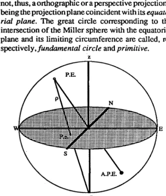
1.1.1. Stereographic Projection

Thestereographic projectioncanbedefined as

the projection of a spherical surface (Miller sphere) on a plane (Fig. 1), where the projectant rays are centered inapoint ofviewplaced in the upper(zenith)

orlower(nadir)poles ofthe sphere of reference (it is not, thus, a orthographic or a perspective projection), being the projection plane coincident with its

equato-rial plane. The great circle corresponding to the

intersection of the Miller sphere with the equatorial plane and its limiting circumference are called,

re-spectively,fundamental circleandprimitive.

z

n

Fig. 1 - Stereographic Projection (perspective of the Miller sphere). z - zenith; n - nadir; P.E. - spheric pole; A.P.E spheric antipole; P.e. stereographic pole; p

-projectant ray.

We can thus represent any point of the spherical surface but the point of view itself in the equatorial plane, connecting the spheric pole to the point of view with a projecting ray, and defining the so obtainedstereographic poleas the intersection ofthe projection ray with the equatorial plane. So, and reporting to the same figure:

-let's consider the sphere of reference split in two hemispheres (upper and lower hemispheres)

separated by an horizontal equatorial plane;

-let's consider, passing by the center of the sphere and at right angles to the equatorial plane, a line, thezenith-nadir line.That line will intersect the sphere in two points, theupperand lower points of view.

Ifwe cross the sphere by any other line, passing by the Center, two antipodal intersections will result,

itsspheric poleand antipole;

- if, on the other hand, we cut the sphere by a plane that also includes its center, an intersection corresponding to a great circle will result, or its

cyclographicrepresentation.

Let's adopt the lower point of view, as normally is the case with this projection (Fig. 2); that way only the part of the geometric elements located on the upper hemisphere willbeof interest to us, otherwise the projections would fall outside the primitive.

Ifwe connect any spheric pole (the cyclographic representation of a plane is also made of points) with the point of view, a new line will result, crossing the equatorialplane somewhere in a point corresponding to the stereog raphic pole,or its stereographic projec-tion.

z

n

Fig. 2 - Stereographic Projection (profile of the Miller sphere); 0 - center of the sphere and projection; R - radius; n - point of view; B(p.E.) - spheric pole; X(p.e.)-stereographic pole;(3-dip of a plane; 11l-angle inscribed in

the complementary of(3.

1.1.2. Lambert projection

In the Lambert(orequal area) projection(Fig. 3), as the lower hemisphere is normally used, the projection plane is tangent to the nadir of the sphere, and the representation of the spheric poles is not obtained by projectant rays but by drawing an arc from the spheric pole to the projection plane, centered in the point of tangence and with radius equal to the distance from that point to the spheric pole. We can thus define theLambertpoleas the intersection ofthe arc so defined with the plane of projection.

1.1.3. Orthographic projection

In the orthographic projection (Fig. 4), using also, hypothetically, the lower hemisphere, the plane ofprojection is also tangent to the nadir ofthe sphere. The orthographic representation of the spheric poles

(theorthographic poles- P.O.) is obtained by the

By those processes one dimension of space can 1.2. Construction of auxiliary projection nets thus be eliminated from any of the geometrical

ele-ments of interest to us (the planes are now repre- 1.2.1. True-angle stereographic net (Wulff net) sented by lines - great circles - and the lines by

points). Nevertheless, they are difficult and slow to

calculate, for which auxiliary projection nets are 1.2.1.1. Equatorial net normally used, as refered.

B Fig. 3 - Lambert projection (profile). 0 - center of the sphere;A - tangency point (center of the projection);R -radius of the sphere (different from the -radius of the projection); B(p.E.) - spheric pole; X(p.L.) -Lambert pole;

f3 -

dip of plane.

X(P.L.) A(n)

This net is composed by two families of curved z lines (great and small circles), drawn from the

projec-___--r-__

_{tion on the equatorial plane of the Miller sphere of}

two such families of planes (Fig. SC).

Projection plane

z

FigA-Orthographicprojection (profile); 0 - center of the sphere; A - Point of tangency (center of the projection); R - radius of the sphere (equal to the radius of the projection); B(p.E.) - spheric pole; X(p.O.) - orthographic pole;

f3 -

dip

of plane.

Projection plane _{A(n) X(P.O.)}

c

Fig. 5 - (A) - Family of great circles, intersecting in a common diameter of the primitive; its stereographic pro-jection defines the meridians of the Wulff net. (B) - Family of apex centered coaxial cones, whose stereographic pro-jection defines the family of small circles in the Wulff net. (C) - Conjugation of the two families defined in (A) e (B).

<\>= (rc/2 -~)/2 => <\>= (rc/4 -~/2) [1]

from which:

This net is also composed of two families of lines, the first straight and radial and the second circular and concentric.

The principle of construction for this net is identical to the previous one, differing only on the following aspects:

1- The family of planes originating the great circles have its common line not on but at right angles to the equatorial plane, passing by its center;

2- The succession of parallel planes originating the small circles is oriented not perpendicularl y to the primitive but parallel to it.

So, the difference between the polar and equato-rial nets consists in a 90° rotation of the planes necessary to their construction, on thefirst case on the common line on the equatorial plane. This line is the N-S line of the projection (Fig. SA).

The arcs for the small circles correspond to the projection of a series of planes cutting the sphere of reference at right angles both to the plane of projec-tion and the aforemenprojec-tioned N-S line. Those planes are so separated as to the centered angles, in the equatorial plane, between the successive radii so defined, differ by the stipulated amount defined for the construction of the net. The plane passing by the center of the sphere of reference will be the onl y great circle of the family, and its projection will be the E-W line of the net.

The surfaces defined by the connection of the center of the sphere with the intersections of the successive planes with the sphere are cones of revo-lution, coaxial and with juxtaposed vertices (Fig. 5B).

In this projection, the shapes are maintained, and all the projected planes are represented by arcs of circumference and the angles are projected in true value. This fact allows us to establish a series of relationships between the great circle of any plane and its stereographic projection on the net.

Let's consider the vertical section of the sphere ofreference (Fig.2), pcrpendicularto any given plane as to represent its true dip(B);the segment OB (the trace of the plane on the section plane) is the radius of the sphere, and the segment OX corresponds to the distance between the great circle of the given plane and the center of the sphere, measured on the funda-mental circle, ofradiusR.The linenBis the projectant line from B (thus connected to the point of view n) passing, necessarily, by X.

So, as the angle OT"TB (<\» is the inscribed angle corresponding to the complementary of the b centered angle, its value is:

1.2.2.2. Polar Net

[3]

[5]

AX =

R.J2,

AX

=

..J'2Rsen(rc/4-p/2) [4] As, for ~ =0°,

AX

=

Rcos (~)

AX= 2R sin (rc/4 -~/2)

so:

N-S line of the projection and on the last on the zenith-nadir line of the sphere of reference; the same is valid for the nets in the other projections.

A vertical section of the reference sphere shows a plane of dip ~ intersecting it in B and passing by its center O. The point X is found projecting B orthogonally to the projection plane, being the dis-tance AX found from the radiusRas:

This expression causes the radius of the primi-tive to be greater than the radius of the sphere, as can be proved making b equal to 0° (the very plane of the primitive). So, to make AX max

=

R, all AX values have to be scaled.

This net is built similar!y to the equatorial Wulff net, although its projection is obtained not by geo-metrical means, but by calculation, as shown in figure3.

A vertical section on the reference sphere shows its intersection (B) with a plane ofdip~ passing by the center O. The projection ofB is made by rotating it to X, on the projection tangent plane, maintaining AX

=

AB. This distance, AX, can be calculated from the radius of the sphere,R as follows:

for any plane of dip~.

This net is constructed the same way ofthe polar equiangular net, differing only in the way its concen-tric circles are scaled (eq. [4]).

The polar nets are presented because, while of more restricted usage, they ease the projection of points. On those nets the rotation of the transparent paper is unnecessary, substantially speeding the pro-jection of a great quantity ofpoint data. As this is their main usc, it is natural that only the polar equal area net is used, as it is the only one adequate to a later statistical treatment on counting nets.

1.2.3.1. Equatorial Net

1.2.3. Orthographic Projection 1.2.2. Equal Area (Schmidt) net

[2]

OX

=

R . tg(rc/4 -~/2)

1.2.3.2. Polar Net

The construction ofthis net obeys the principles of construction of the other two polar nets, the only difference being that the radius of its concentric circles are found through the equation [5].

1.3.

Statistical treatment of point populations

1.3.1. Counting nets

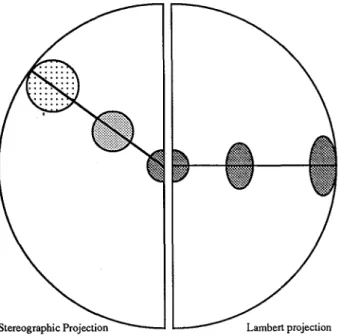
For the statistical analysis of a three dimen-sional population of orientations, such as planes or lines, its projection is necessary on one of the nets described above. Nevertheless, as only the Lambert projection respects the equality of areas and, conse-quently, the density of the distribution on the whole surface, it is natural that this is the projection of choice for this type of analysis.

Lambert projection

Fig. 6 - Comparison between the deformations induced by the stereographic and the Lambert projections.

As we can see in the figure 6, the stereographic projection, while keeping the shapes of equal aper-ture circles undistorted, deforms their area, nearly doubling it from the center to the primitive. On the opposite, the Lambert projection (to which the Schmidt net is associated) respects the equality of areas, even if it has to sacrifice the shape to do so; the spheric circles of equal aperture then change, when projected, to more and more deformed ellipses from the center to the primitive.

Several types of counting nets exist, described by a number of authors, every one of them based on the same principle, the creation of a regular net of counting centers, each one of them taking the value ("weight") of the number ofpoints found in a certain

"area of influence". From the several nets we can refer those of hexagonal symmetry and polygonal area of influence, used by several authors (for in-stance, the Kalsbeek net), those of quadratic symme-try and elliptical area, not very much used now, and sundry nets ofseveral symmetries with circular areas of influence. We chose thistypeas those nets repre-sent, in our understanding, the ones allowing a more correct statistical analysis, attributing to each count-ing center areas of influence represented by small circles of constant radius.

ALVES & MENDES (1972) developed two counting nets (IGAREA 220 and IGAREA 523, numbered from the counting cones used), the first for distributions between one hundred and two hundred points and the second for distributions of a high number of points or smaller distributions of weak concentration. The second net is, from personal expe-rience, seldom used, not only because the number of points lies normally between one hundred and two hundred but also the drawing is so dense that its use becomes very awkward. For that reason the authors separated it in four components, to be used separately and then superposed.

Those nets were calculated admitting a constant angular distance between counting centers, 10° in the case oflGAREA 220 (in annex), the only to be drawn with the program STEGRAPH. We have, then, the counting centers distributed by concentric circles with radii growing by 10° steps from the center, and also separated within each circle by approximately 10°. In practice, to maintain an hexagonal symmetry, chosen by those authors, the number of centers in each "shell" was rounded to the nearest multiple of 6. The radius ofeach "area ofinfluence" is 8°, allowing a sufficient superposition.

II. DRAWING OF NETS

11.1. Equatorial nets

The calculation and drawing of equatorial nets are somewhat difficult due to the fact that both the drawing of great and small circles are made for every point.

Let's consider, then, a great circle correspond-ing to a plane of dip[3(Fig. 7). Whatever its value, it is equal to the plunge of the line of maximum plunge in the plane, represented by a point in the intersection of the cyclographic representation of the plane and the diameter of the primitive perpendicular to the horizontal line of the plane. We have, then, three of its points, corresponding respectivelytothe line of true dip and the two points of intersection of the cyclographic representation with the primitive.

Fig. 7 - Calculations for arcs in equatorial nets.

As we can see from the figure,

b b

tan(~) = and tan(W) =

a c

so then:

b

=

a . tan(/3) e b

=

c . tan(/3')

but as:

a

=

sin(r) c

we have:

tan(/3')

=

sin(y) . tan(/3)

or finally:

f3'

=

tan- l [sin(y) . tan(f3)]. [6]

Then weonlymustperforrn thenecessarycalcu-lations, according to equations[2], [4]and[5](Wulff, Schmidt and orthographic nets, respectively); the calculations must be made for a large enough number of points along the line so that it can be drawn with a minimum of precision. In theSTEGRAPHprogram, for reasons of clarity,the circles ofdip multiple from 10°, besides being drawn with a different colour from the others, are also drawn between the small circles of radius equal to the equidistance of the circles; those not multiple of 10° are drawn, in the Wulff net, between the small circles of radius 10° and, in the Schmidt and orthographic nets, between the small circles of radius 20°.

The problems arising from the drawing of small circles are different from those seen in the drawing of great circles, slightly more difficult but nonethe-less solvable with the help of the spherical trigonom-etry.

Let us consider, then, a small circle of radius a (Fig.7). This circle defines, in the family of great circles whose axis intersects the small circle in its middle arcs of value x

=

90°-o, Admitting that the dips of such great circles are successively known, for instance fixed, by the program, as equal to /3, we can then define a spherical triangle, rectangular in Z, whose sides are x and y and the hypotenuse is z, As in any rectangular spherical triangle the cosinus of the hypotenuse is equal to the product of the cosinus of the sides, we have:

z

=

cos! (cos x . cos y)

Fig. 8 - /3 -True dip ofplane P; /3' -dip of plane P in plane PI;'Y - Angle between the strikes of the plane P and the

sectioning plane Pl.

Il~j~!~~~!I-

Plano P

which follows as:

a . tan(/3)

=

c . tan(/3').

From that we take:

lul-

Planol}

But, in the polar coordinate system used up to this point (where the posi tion of each point is defined by two coordinates, an angle {} and a distance L) z, besides being the hypotenuse of the triangle consid-ered is also the value of the arc corresponding to the distance L, which can be calculated from the equa-tions [2], [4]and [5].

As we can also see, the angle {} is equal to the angle X of the spherical triangle used and, to find its value, we must use another property of the spherical triangles, which states that in any spherical triangle the sinuses of the sides are proportional to the sinuses of the angles they oppose. We have, then:

tan(W) = - .a tan(~) c

sin x sin X

11.2. Polar Nets

11.3. The IGAREA 220 counting net

semi-meridian of reference

b

=

cos-1[cos(a) . cos(c)+sin(a) . sin(c) . cos (B)],

we can see that we can calculate the angle C that, added to the angle D, gives us the coordinate 9 of the point P. For ease of the calculations, we chose to split the drawing in two parts, one where the angle C is considered positive, varying B between 0° and 180°, and repeating the calculations for C as negative. The points where C is equal to 0° (B

=

0° or 180°), corresponding to discontinuities of the curve, are calculated by itself (we cannot, with these points, define a spherical triangle). The circles centered on the primitive are drawn taking in consideration that they cannot extend beyond the circle ofthe primitive. As a comment, we can add that this method can be used for the representation of any circular counting net, with any distribution of the counting centers, needing only their coordinates and the radius of the Fig. 9 - Drawing of small circles by calculating lite

coordinates of all its points.

sin(A) sin(B) sin(C) = = -sin(a) sin(b) sin(c)

we can thus calculate the sideb,which is actually the coordinate L, in degrees, of the pointP:

- by the ratio

between the vector radius of its center and the merid-ian of reference), the polar coordinates(Land9)of any point P, at a set distance from the center, can be_{. ~~.~}

calculated as follows: .

- Admitting a sphericaltriangle with its,,~rti­ ces placed respectivelly on the center of the stereogram, the center of the small circle and the point P, we can define the sidea and the angle D (coordinates of the center ofthe small circle), and the side c(arc between the point P and the center of the small circle);

- Varying then the angle B between 0° and 360°, and knowing that:

[7]

Z

_=arcsm

.

(Sin

z.

sin

X)

sin x

For the counting nets, in the present case the IGAREA 220 net, already described, the process is based on the drawing of small circles of fixed radius (8° in this case) centered on the knots of the net. As the projection employed is the Lambert equal area projection, the small circles are projected as closed 4l1tdegree curves (Fig. 9).

So, the drawing of a small circle depends from a number of factors, among them the coordinates of its center. After they are calculated, thus knowing the position of the circle within the stereogram, the next step involves the calculus ofthe coordinates of all the points at a given angular distance from the center.

Given, thus, a small circle of coordinates a (distance to the center, in degrees) and D (angle Allowing that, obviously, the calculations for the drawing of both the equatorial circle and the great circles (the "meridians" of the Miller sphere) poses no problems (today any drafting plotter has an inter-nal set of instructions allowing the drawing of both straight lines beginning and ending at any point within the drawing area and circles of any radius centered at any point), the drawing ofa small circle is dependent on the ratio between its radius on the sphere (in degrees) and its radius on theprojection (or the ratio between its radius and that ofthe primitive). We thus opted for drawing the net in two steps, the first common to every type of polar net consisting on the drawing of the circle of the primitive, the angular values and the two main great circles (the horizontal and the vertical ones). From this point, by the equations [2],[4]and[5],we calculate the radius ofthe successive small circles, drawing them centered within the circle ofthe primitive. Note that, ifdesired, the primitive and the small circles of radius multiple of 10° can have a different colour, for clarity.

After the small circles, the drawing of the great circles is simple, in this type of net they are repre-sented by straight lines radiating from the center. For clarity, we do not draw them from the center. The multiples of 10° are drawn from the first small circle, and the other are drawn from the 10° small circle.

Varying, with a convenient step, the dip

13

of the great circle, and taking as constant the angle ex, we can calculate the polar coordinates of all the points belonging to the small circle and, with a simple transformation, the orthogonal coordinates used by the drafting plotter.

circles of influence.Inthe present case, we chose not to calculate those coordinates but to have them preset within the program.

11.4. The Ortographic DTP Abacus

By personal suggestion of A. Ribeiro, an ortographic abacus for use in Structural Geology was developed, based on the methods devised by DE PAOR (1983, 1986), and included in the program

STEGRAPH.

This abacus consists of a series of circles pro-jected ortographically on the small circles of an equatorial ortographic net, in order to calculate the deformation occurring along the small circles.

ID. APPLICATIONS (Prog. STEGRAPH, verso

2.0)

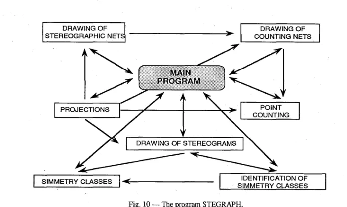
The program STEGRAPH (3) allows us, be-sides the drawing ofthe projection nets, and based on the fact that all the principles subjacent to the several projections are already in it, its use in other applica-tions (Fig. 10).

111.1. Counting of points in the IGAREA

220

net

For the automatic counting of points we need to introduce the orientations of the planes or lines to project in an external text file (ASCII format) then used by the program. The orientations must be placed in consecutive lines, with a space between the two

IDENTIFICATION OF . SIMMETRY CLASSES

DRAWING OF COUNTING NETS

SIMMETRY CLASSES

I...

-<~---DRAWING OF STEREOGRAPHIC NET

Fig. 10 - The program STEGRAPH.

- Planes (The examples refer to the same values, arid several formats can be used simultane-ously:

plane)

Normal notation: 25SW

Azimuthal notation: Dip orientation:

N45W 25SW or S45E

315 25SW or 135 25SW 22525

value associated to each one of them when the angle is equal or less than 8°, by the equation:

a=cos-l [cos (J3) cos (y)+sineJ3)sin(y) cos (A)] [8]

As the operation is processed reading succes-sivelyevery orientation in the text file in the hard disk, the number ofpoints to use is only limited by the size of the hard disk.

- Lines (The examples refer to the same line)

Normal notation: 50 S40W Azimuthal notation: 50 220

Internally all those formats are converted to azimuthal coordinates, easier to use by the program. The counting is made (Fig. 11) calculating the angle (a) between the points included in the file (P) and the centers of the counting net(Q),adding to the

111.2. Deduction of simmetry classes

The existence of this subroutine is linked to a future projection of the stereograms of the various classes, associated with the stereo graphic projection of crystallographic models, to be included futurelly in the program.

AZ2 \ \

\ \

\

_ _---,\P

Fig. 11 - Calculus ofthe angle between two points (P and Q): A - difference between the azimuths of P and Q (= LlAz);

13

and 'Y - Distance, in degrees, to the center

(complementar to the respective dip values).

CONCLUSIONS

The present paper intended not only to demon-strate that the use and drawing of auxiliary projection nets ought nottobe treated as a "hermetic science" but also to allow resolution of problems in the areas of crystallography and structural geology, namely:

I - Applications in Crystallography:

a) Stereographic projection ofcrystallographic models;

b) Stereographic calculations (Miller indexes, for example);

c) Drawing of stereograms of all symmetry classes;

2 - Applications in Structural Geology:

a) Statistical analysis of populations of pro-jected points;

b) Determination ofstress fields from the analy-sis and interpretation of structures.

In its present version, the program STEGRAPH has an essentially pedagogic utilization; with the above mentioned additions, it shall be a tool extend-ing to all the fields where the stereo graphical projec-tion is used.

BIBLIOGRAPHY

ALVES, C.M. & MENDES, F.P. (1972) - Contagem manual de orientacoes.Rev. Cienc. Geol6gicas, Lourenco Marques, Vo1.5, Serie A, pp. 9-17,4 fig.

BEVIS, M. (1987) - Computing relative plate velocities: a primer.Mathematical Geology,New York, Vo1.19, N1l6, pp.561-569, 2 fig., tabl.1.

BORGES, F.S. (1982) - Elementos de Cristalografia. 644 pp.,Fund. C.Gulbenkian.Lisboa.

BRAVO,M.S. _{& MENESES, L.L.(1990) - Cristais a duas dimensoes. 115 pp.,}C.E.P.UNL.(INIC) -(FCTIUNL). Monte de Caparica.

DE PAOR, D. G. (1983) - Ortographic analysis of geological structures -I.Deformation theory.Journal ofStructural Geology,Oxford, vol. 5, nil 3/4, pp. 255-277, 27 fig.

DEPAOR, D. G. (1986) - Ortographic analysis ofgeological structures - II. Practical applications.Journal ofStructural Geology,Oxford, vol. 8, nll1,_{pp. 87-100, 19 fig.}

HINKS,A.R. (1912) - Map projections.Cambridge University Press.Cambridge, 138 pp.

HOBBS, RE., MEANS, W.D.& WILLIAMS, P.F. (1976) - An outline of Structural Geology.John Wiley and Sons, New York, 592 pp..

JAMSA, K. (1989) - Using DOS 4. Osborne McGraw-Hill.Barkeley, 1022 pp.

KULLBERG, M.C. & SILVA, J.B. (1981) - Apontamentos sobre0 uso da projeccao estereografica em Geologia

Estrutural.A.E.F.C.L.Lisboa, 34 pp., 52 fig., 2 tabl.

LIBAULT, A. (1975) - Geocartografia. Companhia Editora Nacional. Sao Paulo, 398 pp.

MORRISON, G.J. (1911) - Maps, their uses and construction. (2' ed.).Edward Stanford.,London, 164 pp. NAMEROFF, S. (1989) - QuickBASIC®, the complete reference.Osborne McGraw-Hill.,Barkeley, 593 pp. PHILLIPS, F.C. (1960) - The use ofstereographic projection in structural geology. (2' ed.).EdwardArnold(Publishers)

Ltd.,London, 94 pp.

PHILLIPS, F.C. (1978) - An introduction to Crystallography. (4" ed.).Oliver Boyd,Edinburgh, 404 pp.

RICHARDUS, P. & ADLER, R.K. (1972) - Map Projections for geodesists, cartographers and geographers. North-Holland Pub. Comp.,Amsterdam, 184 pp.

PROJEC<;AO ESTEREOGRAFICA

REDE DE IGUAL ANGULO DE WULFF

...

,0>

...

t.

Rede equatorial

PROJECCAO DE LAMBERT

REDE DE IGUAL AREA DE SCHMIDT

""

I.

'00

""

,.

Rede equatorial

PROJECC;AO ORTOGRAFICA

'0

Rede equatorial

REDE IGAREA 220

...

170

ABACO ORTOGRAFICO DTP