Recommending media content based on machine learning methods

(1)

Pedro Ricardo Gomes Dias

Licenciado em Engenharia Informática

Recommending media content based on

machine learning methods

Dissertação para obtenção do Grau de Mestre em Engenharia Informática

Orientador : Prof. Doutor João Magalhães, Prof. Auxiliar Convidado, FCT/UNL

Júri:

Presidente: Prof. Doutor Nuno Preguiça

Arguente: Prof. Doutor Francisco Revilla

(2)

(3)

iii

Recommending media content based on machine learning methods

Copyright cPedro Ricardo Gomes Dias, Faculdade de Ciências e Tecnologia, Universi-dade Nova de Lisboa

(4)

(5)

(6)

(7)

Acknowledgements

Elaborating this thesis has been a long and fascinating journey through a path of dis-cipline, hard work, discovery and rewarding sense of accomplishment. I did not walk this path alone, which is why I owe those who supported me throughout this process a sincere and grateful acknowledgement.

To my thesis advisor Prof. Dr. João Magalhães, for his confidence in my work, for his guidance and knowledge sharing, for his flexibility and availability, and for his remark-able ability to keep me highly motivated that made the elaboration of this thesis such a pleasant and rewarding experience.

To my faculty Faculdade de Ciências e Tecnologia da Universidade Nova de Lisboa, in particular to the Informatics Department, for providing an exceptional environment for making science and for leading a high-quality academic life.

To the Immersive TV project in which this thesis is inserted, for granting me a scholarship that helped me carry on with my studies.

To my teachers and friends Prof. Dr. Christopher D. Auretta and Prof. Dr. Ruy Costa, for being such a rich and inspiring example.

To all my university colleagues and friends, in particular Diogo Bernardino, Gustavo Azevedo, João Santos, Márcia Silva, Pedro Ramos Afonso, Sofia Gomes and Tewodros A. Beyene for their friendship and company along the way.

To all my long time friends, in particular André Macedo, Carla Ferreira, Filipe Macedo, Hugo Aguiar and Sofia Canelas for always being there for me and for their unconditional friendship, example and frequent laughters.

(8)

viii

To my father José Dias for supporting and loving me.

To everyone else in my wonderful and generous family for giving me a home.

To my beautiful and graceful girlfriend Agnieszka Kapral, for brightening up my days.

(9)

Abstract

Information is nowadays made available and consumed faster than ever before. This in-formation technology generation has access to a tremendous deal of data and is left with the heavy burden of choosing what is relevant. With the increasing growth of media sources, the amount of content made available to users has become overwhelming and in need to be managed. Recommender systems emerged with the purpose of providing personalized and meaningful content recommendations based on users’ preferences and usage history. Due to their utility and commercial potential, recommender systems inte-grate many audiovisual content providers and represent one of their most important and valuable services. The goal of this thesis is to develop a recommender system based on matrix factorization methods, capable of providing meaningful and personalized prod-uct recommendations to individual users and groups of users, by taking into account users’ rating patterns and biased tendencies, as well as their fluctuations throughout time.

(10)

(11)

Resumo

A informação é hoje em dia disponibilizada e consumida mais depressa do que nunca. Esta geração das tecnologias da informação tem acesso a uma enorme quantidade de diferentes conteúdos, competindo-lhe a árdua tarefa de seleccionar aqueles que são re-levantes. Com o crescente aumento das fontes de informação, a quantidade de conteú-dos disponibilizaconteú-dos aos utilizadores tornou-se avassaladora, surgindo a necessidade da existência de meios que façam a sua gestão. Os sistemas de recomendação surgiram com o propósito de oferecer sugestões de conteúdos personalizadas e pertinentes, baseadas nas preferências dos utilizadores e no seu histórico. Devido à sua utilidade e potencial comercial, os sistemas de recomendação integram diversos fornecedores de conteúdos audiovisuais, representando um dos seus mais valiosos e importantes serviços. O objec-tivo desta dissertação é desenvolver um sistema de recomendação baseado em métodos de factorização de matrizes, capaz de fazer recomendações pertinentes e personalizadas de produtos a utilizadores individuais e a grupos de utilizadores, tendo em conta os seus padrões deratinge respectivos desvios individuais, bem como as suas flutuações ao longo do tempo.

(12)

(13)

List of Figures

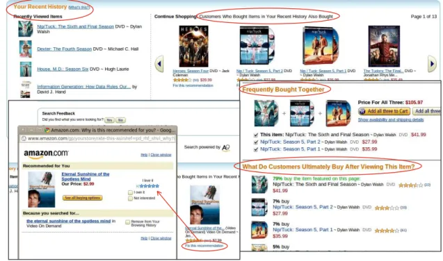
1.1 Amazon recommendations based on a user recent history and consump-tion patterns of similar users.Fix this recommendationfeature. . . 3

1.2 Amazon’s"Today’s recommendations", search and rate feature andlikebutton. 3

1.3 Hulu’s rating scale, demographic data solicitation andImprove Your Rec-ommendationsfeature. . . 4

1.4 Netflix’s search box from which preferences are inferred andOur best guess feature. . . 5

2.1 User-user similarity matrix . . . 12

2.2 Hierarchical clustering algorithm iterations. Illustration taken from [35]. . 16

2.3 Dendrogram visualization of hierarchical clustering. Illustration taken from [35]. . . 17

2.4 Iterations of K-means algorithm. Illustration taken from [35]. . . 17

3.1 Latent factor approach with 2 factors where both users and products are represented under the same feature space. Illustration take from the work of Koren et al. [22]. . . 20

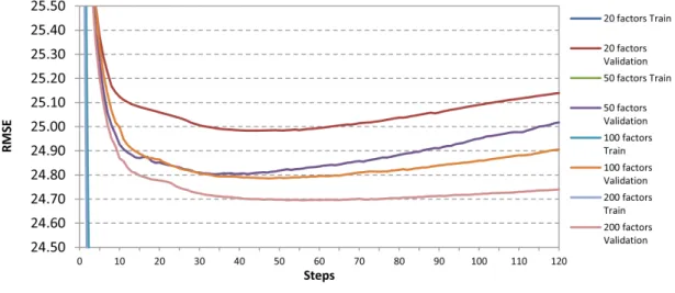
3.2 Plain-SVD model learning behaviour over 120 steps with different num-bers of latent factors . . . 38

3.3 Plain-SVD model learning behaviour over 120 steps with different num-bers of latent factors (zoomed). . . 38

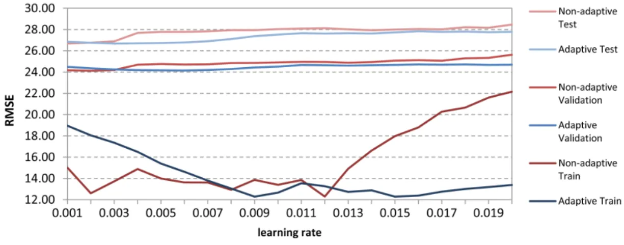
3.4 Plain-SVD model performance with different learning rates. . . 39

3.5 Performance comparison between adaptive and non-adaptive learning rates for the plain-SVD model using 200 factors . . . 40

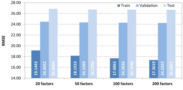
3.6 Performance of plain-SVD model with different numbers of latent factors 41

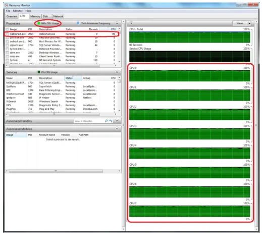
3.7 CPU usage at 8-core parallel processing of the plain-SVD model . . . 42

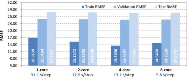
3.8 Performance of plain SVD model with different levels of parallelization . 43

(18)

xviii LIST OF FIGURES

4.2 Bias-SVD model with different learning rates . . . 57

4.3 Temp-SVD model with different learning rates . . . 57

4.4 Performance comparison between adaptive and non-adaptive learning rates for the temp-SVD model using 200 factors . . . 58

4.5 Comparison between plain-SVD, bias-SVD and temp-SVD models . . . . 59

4.6 CPU usage at 8-core parallel processing of the temp-SVD model . . . 60

4.7 Performance of plain-SVD, bias-SVD and temp-SVD models with different levels of parallelization . . . 61

4.8 RMSEs on the test and validation sets throughout the temp-SVD model learning process . . . 62

5.1 Graph of the song playlist production process . . . 64

5.2 Illustration of target users detection and preference combination with group leaders . . . 66

5.3 K-means clustering with different numbers of latent factors. . . 68

5.4 Results of single-group recommendation . . . 73

5.5 Results of 2-group recommendation . . . 74

5.6 Results of 3-group recommendation . . . 74

5.7 Averaged results of all 3 groups of experiments . . . 75

7.1 Results of group rec. with 2 factors, grouped by experiment . . . 87

7.2 Results of group rec. with 2 factors, grouped by nr. of groups involved . . 87

7.5 Results of group rec. with 2 factors grouped by experiment . . . 89

(19)

List of Tables

5.1 Statistics on group recommendation experiments. . . 73

(20)

(21)

1

Introduction

1.1 Recommender systems

This is an information era. Information is nowadays made available and consumed faster than ever before. This information technology generation has access to a tremendous deal of data and is left with the heavy burden of choosing what is relevant. With the increasing growth of media sources, the amount of content made available to users has become overwhelming and in need to be managed. The quality of user experience is thus defined by how this phenomenon is dealt with. Because browsing the wide range of available content is impractical on a user perspective, it becomes crucial to find ways of identifying the small portion of relevant content by searching through all possibilities. The ability to perform such filtering determines the quality and productivity of user experience when interacting with information sources.

(22)

1. INTRODUCTION 1.2. Media marketplaces and consumption

1.2 Media marketplaces and consumption

Recommender systems are offered by the widest audiovisual content providers, such as Amazon video-on-demand (VoD), Hulu or NetFlix, and represent one of their most important and valuable services [11]. The amount of available data involved is enormous due to the millions of users and the millions of products registered on their databases. Most of these systems operate similarly: users are encouraged to give ratings to products and based on those ratings and on any additional information about the users, such as demographic data and search history, products are recommended.

1.2.1 Amazon video-on-demand (VoD)

Amazon is a worldwide online marketplace with millions of registered users and prod-ucts. At Amazon’s VoD section one can easily notice the presence of a recommender system after performing a few searches for content or just navigating through and visu-alizing some of the available products. Recommendations based on this kind of search and navigation history, referred to asimplicit user feedback, are made to the user from the first interactions with the system. Figure1.1shows an example of product recommenda-tions based on the lists of products recently viewed by the user.

(23)

Figure 1.1: Amazon recommendations based on a user recent history and consumption patterns of similar users.Fix this recommendationfeature.

Figure 1.2: Amazon’s"Today’s recommendations", search and rate feature andlikebutton.

1.2.2 Hulu

(24)

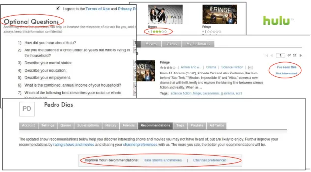
viewed monthly during 2010. The recommender system integrated in Hulu website ap-plies user feedback and profile characteristics to make recommend products. Upon regis-tering, the user is asked to introduce some optional personal information such as marital status, annual income or ethic background, as shown on Figure 1.3, that will be used to set up a user profile, thus adding some content-based methodologies to the recom-mendation algorithm used to make product suggestions. Like many other collaborative filtering recommender systems, Hulu is based mostly on user feedback to compute pre-dictions about what products the users will like. Users can give their explicit feedback by giving ratings to products in a scale that ranges from 1 to 5. Additionally, users can ex-plicitly inform the system about which videos they have already watched or which ones they simply have no interest in, as Figure1.3illustrates, allowing for the system to know more about users’ preferences. Moreover, on the user personal area there is a recommen-dations tab on which the user gets the solicitation Improve Your Recommendations, being then led to rate more products or manifest channel preferences, as shown on Figure1.3.

Figure 1.3: Hulu’s rating scale, demographic data solicitation and Improve Your Recom-mendationsfeature.

1.2.3 Netflix

(25)

1. INTRODUCTION 1.3. Problem definition and thesis objective

as illustrated on Figure1.4.

Figure 1.4: Netflix’s search box from which preferences are inferred andOur best guess feature.

1.2.3.1 Netflix prize

In 2006 Netflix held a contest offering 1 million dollars to anyone who could create a col-laborative filtering recommendation algorithm that would surpass their own - by then namedCinematch - in terms of prediction accuracy by at least 10%. Only 3 years later the team BellKor’s Pragmatic Chaos, which was a fusion between several teams initially competing for the prize individually, accomplished such deed. Every team had available to train and test their algorithms around 100 million ratings given by more than 480,000 users to almost 18,000 movies. The fact that Netflix was willing to pay such amount of money for a recommender algorithm stresses how valuable and important good recom-mendations are for the success of this kind of business.

1.3 Problem definition and thesis objective

(26)

1. INTRODUCTION 1.3. Problem definition and thesis objective

Millions of users×Millions of products=Trillions of data to work on

Consumption patterns can be inferred from this information and users may share similar consumption habits among each other. Simplified, if somehow users can be matched according to consumption patterns and preference similarities they can be reliable advice-givers to each other.

Once both users and products are conveniently characterized recommendations can be made using different methods:

• Content-based methods, in which the characteristics inherent to products and users are explored to assess similarities, and recommendations are made according to those similarities;

• Collaborative methods, in which the users’ previous purchases and consumption habits are explored, and recommendations are made based on that;

Within an interactive TV project, there is the need to assess each user’s individual prefer-ences to provide a service as personalized as possible that fits their needs and, by doing so, stimulate consumption. Providing such service involves making personalized prod-uct recommendations with a good degree of accuracy.

The accuracy of the recommendation system depends on the available data to work on and the methods used to combine this data so that recommendations can be then pro-duced. To do so, several different methods involving content-based and/or collaborative filtering must be experimented and analysed, and the extent to which these may be fit for this specific problem and environment must be determined. This can only be done af-ter achieving an understanding about the surrounding environment and its actors: users and products.

Users are the main actors in the system, since they are the consumers and the data providers. Users can be defined by two main classes of attributes:

• Demographic data, which includes every personal information such as age, gender, nationality, area of residence, marital status, ethnic background, average income, etc. This kind of data should be mapped onto numerical values so it can be pro-cessed. As an example, MovieLens stores the ages of users in age groups identified by a number(ex.: 1: 18-24; 2: 25-34). Not all this data is always provided by users but, whenever available, it can be used to complement collaborative algorithms with content-based features.

• Preferences, which can be explicitly expressed to the system through product ratings, or inferred from history of visualized and/or searched products and from user’s consumption habits.

(27)

1. INTRODUCTION 1.4. Contributions

dimensions of the referential on which products are characterized may change. Products will then be represented by the extent to which they fit in each of the referential dimen-sions (ex.: how funny, how reflexive, how scary), mapped onto numerical values, like coordinates on a map.

The relation between a user and a product is defined by the extent to which that user likes that product. This relation can be easily determined when the user rated the product, and its representation is simple: a value, usually between 1 and 5. However, most of the times there are no ratings relating users to products. In this cases, the system shall try to predict the rating a user would give to a product. By doing so, the system is then able to recommend products that the user will probably like. The best techniques and methods to achieve that may differ, but the latest studies show that the most successful approaches to this kind of problem involve matrix factorization methods. Moreover, preferences evolution over time and the ability to infer preferences through implicit feedback also contribute to improve the quality of predictions.

Thus, the objective of this thesis is:

to develop a recommendation algorithm based on (i) the collaborative ratings of products, (ii) the rating biases associated to users and products, (iii) the

temporal fluctuations of ratings and (iv) group preferences.

To accomplish this objective, a baseline matrix factorization model shall be implemented based on the ratings given to products by users. This model must then be improved by adding information accounting for user-related and product-related rating biases. The baseline model shall be further improved by contemplating temporal fluctuations of rat-ings, through inference of rating pattern changes over time. Finally, matrix factorization methods will be combined with clustering methods to provide group-based recommen-dations.

1.4 Contributions

The contributions of this thesis are:

• A software package implementing matrix factorization based collaborative filtering techniques for recommender systems, using a Stochastic Gradient Descent (SGD) learning algorithm with optional parallel computation. This implementation also contemplates the use of rating biases and temporal fluctuations, inpired by Y. Ko-ren’s work [20].

• A software package implementing a group-based recommendation framework. The design and architecture of this framework was also proposed by me.

(28)

1. INTRODUCTION 1.5. Organization

The matrix factorization implementation described in this thesis produced results that ranked me among the top7%teams of the Yahoo! SIG-KDD CUP 2011.

1.5 Organization

The rest of this thesis is organized as follows:

• Chapter 2: Related work overview addressing the topics of data representation, similarity metrics, group discovery and recommendation algorithms and techniques.

• Chapter 3:Matrix factorization methods and associated computational constraints, implementation challenges and evaluation.

• Chapter 4:Embedding rating biases and temporal dynamics to the matrix factoriza-tion methods and associated computafactoriza-tional constraints, implementafactoriza-tion challenges and evaluation.

• Chapter 5: Group-based recommendations combining matrix factorization with clustering techniques and respective evaluation.

(29)

2

Background and related work

2.1 Introduction

Recommender systems emerged with the intent of tackling the problem of multimedia content overload and provide meaningful recommendations. Recommender systems have gained noticeable popularity for the past few years, partially due to the Netflix Prize contest held by Netflix - an online DVD rental company - in 2007, awarding with $1M the first team to outperformCinematch(Netflix’s recommender system) with a 10% accuracy improvement. It was not before 2 years later that the team Bellkor’s Pragmatic Chaos finally achieved this goal. More recently, Yahoo held the recommender system contest KDD Cup 2011 on which hundreds of contestants competed to reach the top scores, i.e. to produce user rating predictions with the lowest possible error, stressing the value of this research field.

2.2 Recommendation techniques

Recommender systems rely on two main categories of methods: Content-based filtering andCollaborative filtering. The two mentioned categories of methods will be further ad-dressed in 2.2.1 and 2.2.2, respectively. Additionally, there are Hybrid Approaches that combine both the aforementioned methods in different ways:

• Producing content-based and collaborative recommendations separately and then combining the individual results;

(30)

2. BACKGROUND AND RELATED WORK 2.2. Recommendation techniques

• Setting up a model which inherently incorporates both content-based filtering and Collaborative Filtering methods.

All these categories of methods have been extensively explored and compared through-out the years. G. Adomavicius et al. [1] and Melville et al. [27] presented useful surveys on the matter, where they classified methods, compared approaches and pointed out lim-itations.

2.2.1 Content-based filtering

Content-based filtering approaches aim at exploring users’ and products’ inherent char-acteristics to produce recommendations. These approaches have their roots in text pro-cessing applications [32] and information retrieval [2], where content is mostly textual. When taking this approach towards recommender systems, users and products cannot be seen as atomic elements. Instead, these need to have a more descriptive representation, such as

ui = (ui1, ui2,· · · , uim) and pj = (pj1, pj2,· · · , pjn),

whereui represents useriand the elements fromui1touimrepresent them

characteris-tics of useri. Similarly,pjrepresents productjand the elements frompj1topjnrepresent then characteristics of productj. These characteristics can be gender, nationality, age, genres of music, names of directors, etc., depending on the context and purpose of the recommender system, and can be interpreted as keywords to describe a user or a prod-uct. Based on these characteristics, similarities between users or products can be assessed and used to produce meaningful recommendations. Content-based approaches rely on the assumption that similar users like the same products and that users that consumed a given product will also like products similar to the one consumed. However, some limitations exist when recommending products through content-based filtering, such as the need for accurate - but general enough - descriptions of users and products, without which realistic comparisons are difficult. Another limitation of this approach, referred to asoverspecializationin [1], lies in the fact that users are bound to only get recommenda-tions of products with similar characteristics to those they have consumed before.

2.2.2 Collaborative filtering

(31)

(32)

2.2.2.1 Neighbourhood models

Neighbourhood models try to infer user preferences based on the preferences of like-minded users. The most commonly applied neighbourhood method is the k-nearest-neighbours (k-NN), which can be either user-oriented or item-oriented. On a user-oriented approach rating predictions for a user are calculated as a weighted average of the ratings given by thekusers most similar to the target user. Similarities between users are calcu-lated according to their product ratings and can be represented on a symmetric user-user similarity matrix:



 

1 _{· · ·} s1,m

..

. 1 ...

sn,1 · · · 1 

 

Figure 2.1: User-user similarity matrix

Eachsu1,u2 value on the user-user similarity matrix represents a similarity score between usersu1andu2for all m users in the system. Higher values correspond to higher sim-ilarities and lower values correspond to lower simsim-ilarities. The item-oriented approach [33,41] works analogously to the user-oriented approach: similarities between products are measured and represented on an item-item similarity matrix. Then, rating predic-tions are calculated as a weighted average of the ratings given by the target user to thek

products, within the set of products rated by the user, that are more similar to the target product. This approach has been preferred by web-based companies such as Amazon[23] for being more scalable and allowing for a better explanation of the obtained results, since recommendations are made based on comparisons between products that the user knows and consumed, instead of comparisons with users unknown to the target user. There are several possible similarity metrics suggested in the literature [33,37], which will be fur-ther addressed in section2.3. Once defined the similarity metric to be used within a k-NN method, product rating predictions are given by

ˆ rui=

P j∈Sk

(iu₎sij·ruj P

j∈Sk (iu)sij

, (2.1)

whereS₍k_iu₎is a set with thekproducts rated by useruthat are more similar (i.e., have a higher similarity score according to the adopted similarity metric) to producti,sij is the

similarity score between productsiandjandruj is the rating given by useruto product

(33)

2. BACKGROUND AND RELATED WORK 2.3. Similarity metrics

2.2.2.2 Latent factor models

Latent factor models emerge as an attempt to represent users and products under the same feature space. Applications of such approach include neural networks [31], la-tent dirichlet allocation [5] and Singular Value Decomposition (SVD) [34]. The principle underlying latent factor approaches is that both users and products can be represented under a common reduced dimensionality space of latent factors that are inferred from the data and explain the rating patterns. Chapter 3 will provide a thorough clarifica-tion of the latent factor approach. Individually, latent factor approaches have proven to yield better results than any other methods in terms of predictive accuracy, as the liter-ature produced during the Netflix Prize competition shows. Nevertheless, the winning solution of the Netflix Prize [19] resulted from a combination of the output generated by different collaborative filtering methods, obtained through well-established blending techniques [13].

2.3 Similarity metrics

To determine similarity scores between users, a metric that returns a numerical value to work with must be defined. The similarity metrics most commonly used to compare users are addressed in this section.

2.3.1 Pearson correlation coefficient

The most widely used similarity metric is the Pearson correlation coefficient [36], which measures the extent to which two variables are linearly dependent. In a context where the goal is to find similarities between users based on their item ratings, it can be defined by:

simab=

P j∈I

(raj−r¯a)(rbj−r¯b)

r_P

j∈I

(raj₋¯ra)2 P j∈I

(rbj₋rb¯)2 (2.2)

whereI is the set of items rated by both useraand userb,raj is the rating given by user

ato itemj,rbjis the rating given by userbto itemjandru¯ is the average rating given by useru.

Pearson correlation coefficient has the advantage of dealing with the problem that comes from different users having different rating scales, which could lead to misinterpretations about user preferences similarities. This problem is addressed by subtracting the average ratingru¯ from each item ratingruj.

2.3.2 Cosine similarity

(34)

2. BACKGROUND AND RELATED WORK 2.4. Group recommendation

similarity defined by:

simab = cosra, ~~ rb = ~ ra_·r~b

kra~_k2_{× k}rb~_k2 (2.3)

To calculate cosine similarity, there can be no negative ratings and items left unrated are treated as having a rating of zero. This is not a problem when the set I contains only items rated by both users being compared and the rating scale does not allow ratings below zero. However, empirical studies have proven Pearson correlation coefficient to usually have better results than cosine similarity [6].

2.3.3 Tanimoto coefficient

Tanimoto coefficient is a measure of similarity between two sets. It returns a ratio be-tween the intersection and the union of two sets, thus showing how much two sets have in common comparing to what they don’t. It is defined by:

sima,b= |a∩b| |a_∪b_| =

|a_∩b_|

|a_|+_|b_{| − |}a_∩b_| (2.4)

where |a_|and |b_| represent the number of elements in set aand in set b, respectively,

|a_∩b_|is the number of elements common to set a and setb and |a_∪b_| is the number of elements within the union between setaand setb. The similarity score between two sets obtained with Tanimoto coefficient ranges from 0 (no elements in common) to 1 (all elements in common). This similarity metric is particularly useful when comparing two users based on attributes with binary value. For example, if the feedback given by two users about items within a set is limited to like/don’t like ratings, or if the comparison between two users is based on whether they bought or didn’t buy items within a set, then Tanimoto coefficient would be a good candidate for measuring similarities. The real-world applications for this similarity metric are mostly group discovery methods.

2.4 Group recommendation

Although recommender systems have recently attracted a lot of attention from the sci-entific community, group recommendation has not been widely addressed, since most recommendation techniques are oriented to individual users and focus on maximizing the accuracy of their preference predictions. A. Jameson et al. [14] conducted an enlight-ening survey in 2007 presenting the most relevant works on the field of group recom-mendation, as well as the most common issues addressed by the authors of the surveyed group recommender systems.

(35)

deal with these challenges.

In 2002, the Flytrap system was proposed by A. Crossen et al. [7], presenting a simple system designed to build a soundtrack that would please all users within a group in a tar-get environment. In Flytrap system, user preferences were obtained by registering what they listen to on their private computers, in an implicit fashion. Recommendations were then computed by comparing songs within the system database to those listened to by the group members based on artist and genre. Songs whose artist or genre are known to please more users within the target group were then more eligible to be recommended automatically, without the user having any control over what’s being recommended. The content-based nature of recommendations provided by Flytrap is a constant in most group recommender systems described in literature.

A similar approach was taken in the system CATS (Collaborative Advisory Travel Sys-tem) by McCarthy et al. [26]. CATS is a system designed to recommend travel packages to groups of users. It relies on a form of user feedback namedcritiquing, which consists in having the group users give their real-time opinion about some features associated with the recommended products in amore of this / less of thatfashion. For example, when presented with a travel package recommendation a user can let the system know about his preference for a cheaper or shorter plan, without specifying price or duration values. This user feedback is recorded and linearly combined between all users within the group to be afterwards compared against the set of features that represent each travel package. The CATS systems can then recommend the travel packages that suit better the groups’ critiques.

Another example of group recommender systems is the system Bluemusic proposed by Mahato et al. [24]. In this system users are detected via bluetooth and the awareness of their presence has direct influence on a playlist which is being played on a public place. To be taken into account, a user must register his preferences beforehand. The concept introduced by the Bluemusic system is very simple but introduces an interesting alter-native for incorporating transient awareness of user presences into a real-time playlist recommendation scenario.

2.4.1 Discovering groups

(36)

2.4.1.1 Hierarchical clustering

Hierarchical clustering [35] consists on continuously merging the two most similar groups until all groups are merged. A group can contain a single item and the algorithm starts with each item belonging to a different group. Similarity between groups is measured by the distance that separates them, which is calculated according to a given similar-ity metric (see Section 2.3). The algorithm, illustrated with a 5-item example by Figure

2.2, stops its iterations when there is only one group left. Depending on the application, hierarchical clustering can be applied to find groups of similar items or users.

Figure 2.2: Hierarchical clustering algorithm iterations. Illustration taken from [35].

As the example illustrated by fig. 2.2shows, itemsA,B,C,DandEare initially placed in a 2D space according to their characteristics and stand as individual groups. After the first iteration of the hierarchical clustering algorithm, items AandB are merged into a single group, since their proximity to each other was higher than the proximity between any other pair of groups, which were single items, at that point. After the second itera-tion, the group composed by itemsA andB is merged with the group containing item

C, following the same reasoning on the first iteration. This process continues until there is only one group containing all items, as illustrated by the result of the final iteration on fig.2.2.

(37)

Figure 2.3: Dendrogram visualization of hierarchical clustering. Illustration taken from [35].

2.4.1.2 K-Means clustering

K-Means method [35] algorithm starts with a predefined number of clusters, which is based on the structure of the data. K-Means algorithm begins with randomly placing k centroids. A centroidis a point in space that represents the center of a cluster. After placing allcentroids, the items, that are also placed in space according to their attributes, are assigned to the nearestcentroid. Allcentroidsthen move to the average location of their assigned items and the assignments are redone. This process repeats until all centroids stop moving over iterations.

Figure 2.4: Iterations of K-means algorithm. Illustration taken from [35].

Fig.2.4illustrates an example of K-Means clustering with 5 items and 2 randomly placed centroids. In this example, the items A, B, C, Dand E are placed on a 2D space and 2 centroids, represented as small dark circles, are randomly placed in that same 2D space. After the first iteration the items are assigned to their closestcentroid, resulting in items

AandBbeing assigned to onecentroidand itemsC,DandEbeing assigned to the other one, as shown in the second of the 5 scenarios illustrated by fig. 2.4. Once all items are assigned to the closestcentroid, eachcentroidis moved to the average location of the items assigned to it. The items are then reassigned tocentroidsaccording to thecentroids’ new location, resulting in itemsA,BandCbeing assigned to onecentroidand itemsDandE

being assigned to the other one, as shown in the third scenario. As one can observe, item

(38)

2. BACKGROUND AND RELATED WORK 2.5. Summary

process continues until thecentroidsno longer change location.

2.5 Summary

In this chapter was discussed:

• how data must be represented, specifically users, products and ratings, so that it can be dealt with while performing recommendation algorithms;

• what similarity metrics can be used to measure similarities between products or users;

• what are the main algorithms for discovering groups of products or users;

(39)

3

Recommendations by matrix

factorization

3.1 Introduction

Matrix factorization is a class of linear algebra operations for decomposing matrices that can be used in collaborative filtering. Within the context of recommender systems, matrix factorization techniques are intended to be applied over a user-product ratings matrix where ratings given by users to products are stored, as illustrated by matrixRin3.1.

R= 

  

r11 · · · r1i

..

. . .. ...

ru1 · · · rui 

  

(3.1)

Here, eachrui value in the matrix represents a rating given by useru to producti, ex-pressed by a real value. Matrix factorization techniques have become attractive in the last few years for its accuracy and scalability, and hold nowadays an indisputable place at the top of the most successful techniques for recommender systems [19,38,3,29,22,40]. A thorough explanation regarding the goal of applying matrix factorization to the user-product ratings matrix, as well as the decomposition it pursues and methods for ob-taining such decomposition, are within the scope of this chapter and will be further ad-dressed from section 3.2 onwards. Before looking into matrix factorization with more detail, let us revisit some important underlying concepts, introduced earlier in 2.2.2.2: latent factor approaches.

(40)

3. RECOMMENDATIONS BY MATRIX FACTORIZATION 3.1. Introduction

of latent factor approaches. Within collaborative filtering techniques, latent factor ap-proaches are popular for their accuracy. The purpose of latent factor apap-proaches is to infer implicit latent factors from a dataset that help explaining user-product interactions within the system. The goal of inferring these latent factors is to enable the mapping of both users and products onto the same latent factor space, representing these as vectors withkdimensions:

pu= (u1, u2,· · ·, uk) (3.2)

qi = (i1, i2,· · ·, ik) (3.3)

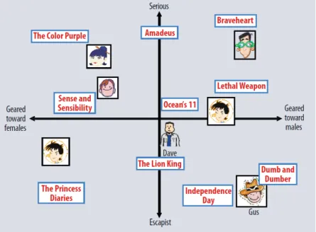
Here,puis the userufactors vector,qiis the productifactors vector andkis the number of latent factors (dimensions) upon which each useruand each productiare represented. By representing users and products in such way, one can evaluate the extent to which users and products share common characteristics by comparing their k factors against each other. Koren et al. [22] presented a visual explanation for the motivation underlying the latent factors approach applied to a context where products are movies, which is an intuitive clarification of its intent, illustrated by fig. 3.1. On the example illustrated by

Figure 3.1: Latent factor approach with 2 factors where both users and products are rep-resented under the same feature space. Illustration take from the work of Koren et al. [22].

(41)

3. RECOMMENDATIONS BY MATRIX FACTORIZATION 3.2. Matrix factorization

interpretation. The goal of such approach is to enable the assessment of user preferences for products by calculating the dot product of their factor representations, as defined by eq.3.4:

rui=pu_·qi, (3.4)

Here,ruiis the preference of userufor producti, both represented as vectors as described in 3.2 and3.3. For example, by observing the placement of users and products on the factors map in Fig.3.1let us assume that the user "Gus" is represented by

pGus= (GustoM ales, Gusserious) = (4,−4) (3.5)

and the movie "Braveheart" is represented by

qBraveheart= (BravehearttoM ales, Braveheartserious) = (4,5) (3.6)

Although both userGusand movieBraveheartscore high on the "Geared toward males" factor, their "Serious" factors set them apart in terms of compatibility. As can be observed, Gus is very fond of "Escapist" (in opposition to "Serious") movies, as expressed by the

−4value on the "Serious/Escapist" axis, whileBraveheartis definitely a "Serious" movie, since it scores5on the "Serious/Escapist" axis. This means that while the "Geared toward males" factor ofGusandBraveheartsuggestsGuswill likeBraveheart, the "Serious" factor suggests precisely the opposite. Thus, according to Eq. 3.4,Guspreference forBraveheart is:

rGus,Braveheart=pGus·qBraveheart= (4,−4)·(4,5) = 4×4 + (−4)×5 =−4 (3.7)

Such prediction indicates thatBraveheartwould not be a good suggestion to present to Gus, which is consistent with our intuition onGus andBraveheart. This example shows the utility of such vector representation of users and products. This chapter shall thus pursue such representation through matrix factorization techniques.

3.2 Matrix factorization

(42)

decomposing the ratings matrix into a 2-matrices representation, as in eq.3.8:

R=P_·QT _⇔ 

  

r1,1 · · · r1,n

..

. . .. ...

rm,1 · · · rm,n     =    

u1,1 · · · u1,k

..

. . .. ...

um,1 · · · um,k    ·    

p1,1 · · · p1,k

..

. . .. ...

pn,1 · · · pn,k     T (3.8)

Here, matrixRis the ratings matrix as defined in3.1. Each vector (row)puofPrepresents

a useruas in3.2, and each vector (row)qiofQrepresents a productias in3.3. Thus, the decomposition suggested by3.8directly relates to the desired preference representation defined in3.4.

3.2.1 Matrix decomposition fundamentals

This subsection followed the discussion presented by Manning et al. in Introduction to Information Retrieval, chapter 18 [25].

Before introducing the technique which will be the baseline for our final implementation, let us review the fundamentals of matrix decomposition and linear algebra supporting it. The matrix factorization technique on which our implementation is based isSingular Value Decomposition(SVD) - an extension ofsymmetric diagonal decomposition. Before look-ing into SVD, let us address two other matrix decomposition techniques named eigen decomposition andsymmetric diagonal decomposition, on which SVD is based. Both these techniques apply to square real-valued matrices only and the latter applies to symmetric matrices only. All three mentioned matrix decomposition techniques rely on the concepts ofeigenvaluesandeigenvectors.Eigenvaluesare the values ofλthat satisfy

R~u=λ~u, (3.9)

whereRis aM _×N matrix and~uis a non-zeroM-vector. Accordingly, theM-vectors~u

satisfying3.9are calledright eigenvectorsofRand theM vectors~vsatisfying

~vTR=λ~vT (3.10)

are called theleft eigenvectorsofR. IfRis a symmetric matrix, theeigenvectors correspond-ing to distincteigenvaluesare orthogonal. Thesymmetric diagonal decompositionis defined by theorem1.

Theorem 1. Symmetric diagonalization: Let R be a square, symmetric real-valuedM_×Mmatrix withM linearly independent eigenvectors. Then, there exists asymmetric diagonal decompo-sitionR=QΛQT _{where the columns of}_Q_{are the orthogonal and normalized (unit length, real)}

eigenvectors ofR, andΛ is the diagonal matrix whose entries are the eigenvalues ofR. Further, all entries ofQare real andQ−1 ₌_QT_.

(43)

3. RECOMMENDATIONS BY MATRIX FACTORIZATION 3.2. Matrix factorization 3.11.      =      ·    λ λ λ   ·       (3.11)

TheΛdiagonal matrix containing theeigenvaluesλofRis usually represented by omitting its non-diagonal values - since these are all zeros - as adopted on eq.3.11.

Definition: It is important to introduce the concept ofrank. Therankof a matrix is the number of linearly independent rows or columns in it. Thus, rank(R) _≤ min_{M, N_}. Moreover, the number of non-zeroeigenvaluesofRis at mostrank(R).

3.2.2 Singular Value Decomposition

The most popular and widely adopted latent factor approach for recommender systems isSingular Value Decomposition (SVD), which is a method for performing matrix factor-ization. SVD is an extension of the aforementioned matrix decomposition technique sym-metric diagonal decomposition[25]. Unlikeeigen decompositionandsymmetric diagonal decom-position, SVD can be applied to non-square matrices. As one can intuitively assume, ifR

is a user-product ratings matrix, only in rare casesM = N, i.e., the number of users is rarely equal to the number of products. The original SVD formulation is:

R=UΣVT = 

  

u11 · · · u1m

..

. . .. ...

um1 · · · umm    ·     λ . .. λ    ·    

v11 · · · v1n

..

. . .. ...

vn1 · · · vnn     T (3.12)

Here, theλ1,· · ·, λreigenvaluesofRRT are the same as theeigenvaluesofRTR. The

orig-inalM _×N matrixR is decomposed to be represented as the dot product between the matrixU, the diagonal matrixΣ, and the transpose of matrixV. These matrices are:

• U:aM_×M matrix whose columns are the orthogonaleigenvectorsofRRT_;

• V:aN _×N matrix whose columns are the orthogonaleigenvectorsofRT_R_;

• Σ: aM _×N matrix where theΣiipositions contain allsingular valuesσi =√λi for i _∈ [1, r]with λi ≥ λi+1 andr = rank(R), and the remaining Σij positions with i₆=jare zeros.

(44)

represented as expressed by eq.3.13.

Σ =          σ1 . .. σr

0 0 0

         (3.13)

As mentioned above, theσi values are called singular values, the M columns contained in U and theN columns contained in V are calledleft singular vectorsandright singular vectors, respectively. Eq.3.14exemplifies such decomposition for a3_×4matrix.

"

5 2 4 6 0 3 1 7 2 6 3 8 #

= "

−0.544 −0.806 −0.234 −0.475 0.526 −0.705 −0.691 0.273 0.669

# ·

"

15.183 0.000 0.000 0.000 0.000 4.392 0.000 0.000 0.000 0.000 1.785 0.000 #

· 

 

−0.270 −0.439 −0.311 −0.798 −0.793 0.365 −0.428 0.235

0.095 0.802 0.206 −0.553 −0.254 −0.467 −0.713 1.000



 

(3.14) As observed, havingr =rank(R), theN ₋r rightmost columns of matrixΣcontaining thesingular valuesofRare filled with zeros. Again, this happens when the decomposed matrix is not a square matrix. Similarly, ifM would be greater thanN, the bottomM₋ r rows of Σ would be filled with zeros instead. For this reason, theΣ matrix is often presented in areducedortruncatedr_×rform, containing only the rows and columns that are necessary to represent the singular values. Accordingly, any rows or columns inU

and V corresponding to the zero-valued rows or columns in Σare also left out in the reduced/truncatedrepresentation of SVD. Additionally, it is important to notice that since

σi ≥ σi+1,singular valuesare progressively less relevant to (i.e., have smaller impact on) the result of the final matrix product. This is a key fact for the dimensionality reduction discussion introduced in the next subsection.

3.2.3 Low-rank dimensionality reduction

In large-scale recommender systems, the ratings matrix can easily contain many millions of entries which makes it a computationally expensive task to compute and even to store its SVD representation. Thus, reducing the dimensionality of the ratings matrix is useful to tackle this problem. Low-rank dimensionality reduction consists in pursuing an ap-proximation of a matrix while reducing itsrank. Given aM _×N matrixRthe goal is to find an approximationRkto matrixRwhoserankis at mostk.

Let us revisit the example introduced by eq. 3.14, now represented in itsreduced/truncated form:

R= "

5 2 4 6 0 3 1 7 2 6 3 8 #

= "

−0.544 −0.806 −0.234 −0.475 0.526 −0.705 −0.691 0.273 0.669

# ·

"

15.183 0.000 0.000 0.000 4.392 0.000

0.000 0.000 1.785 #

· "

−0.270 −0.439 −0.311 −0.798 −0.793 0.365 −0.428 0.235

0.095 0.802 0.206 −0.553 #

(45)

3. RECOMMENDATIONS BY MATRIX FACTORIZATION 3.3. A matrix factorization model

out the less relevantsingular valueofΣ, in this case the one with value1.785, thus reducing dimensionality fromrank= 3torank= 2, leading to:

Rk=2= "

−0.544 −0.806 −0.234 −0.475 0.526 −0.705 −0.691 0.273 0.669

# ·

"

15.183 0.000 0.000 0.000 4.392 0.000

0.000 0.000 0.000 #

· "

−0.270 −0.439 −0.311 −0.798 −0.793 0.365 −0.428 0.235

0.095 0.802 0.206 −0.553 #

(3.16) As we can observe, the resulting matrixRk=2would be a reasonable approximation toR:

Rk=2 = "

5.037 2.334 4.084 5.760 0.115 4.009 1.254 6.298 1.882 5.043 2.750 8.654 #

≈ "

5 2 4 6 0 3 1 7 2 6 3 8 #

=R (3.17)

A measure for assessing the quality of the obtained approximation is theFrobenius norm, addressed in [25], defined as:

kX_kF = v u u t M X i=1 N X j=1

X_ij2 (3.18)

Here,X = R₋Rk, whereR is the original full matrix decomposition andRk is a

low-rank approximation toR. TheFrobenius normof the low-rank approximationRk=2using low-rank dimensionality reduction method would then be:

kR₋Rk=2kF = "

−0.037 −0.334 −0.084 0.240 −0.115 −1.009 −0.254 0.702 0.118 0.957 0.250 −0.654

# F

≈1.784 (3.19)

The Eckart-Young theorem, revisited in [25](Theorem 18.4), shows that this method of dimensionality reduction results in the matrix ofrankkwith the lowest possibleFrobenius error.

3.3 A matrix factorization model

As explained in previous sections, SVD allows to obtain low-rank approximations toR

by zeroing out the less relevantsingular valuesin matrixΣand recalculating the product

U _·Σ_·VT _{with the new lower-rank matrix}_Σ_{. With the appropriate modifications, SVD}

seems to be an appealing choice for pursuing the 2-matrices decomposition of the ratings matrix defined by 3.8, leading to the pursued preference representation introduced by

(46)

3. RECOMMENDATIONS BY MATRIX FACTORIZATION 3.4. Learning the factorization model

ratings matrix, since there are many unknown values which cannot be treated as zeros. Treating the unknown values as zeros would lead to severe inaccuracies, since assuming ratings to be zero is merely blind guessing. Thus, the Frobenius norm is now modified by taking into account only the known ratings, leading to eq.3.20:

kX_kF = s

X

rui∈R

(rui−pu·qTi )2 (3.20)

The second question that must be addressed is related to the fact that, accordingly with eq. 3.4 it is intended to obtain a 2-matrices decomposition ofRinstead of a 3-matrices decomposition as provided by the original SVD technique. As mentioned in subsection

3.2.2, SVD is performed over a matrixRto obtain the decompositionR = UΣVT_{. Since}

our goal is to obtain a decomposition that results in the product of a users matrix and a products matrix, the need to obtain aR =P _·QT _{decomposition leads to the}

factoriza-tion of theΣmatrix into a product of its square roots, so that its square root values get symmetrically blended into the U andV matrices to produce the pursued usersP and productsQmatrices. Eq.3.21formalizes this transformation.

R=UΣVT =U√Σ_·√ΣVT =P_·QT (3.21)

Here,P =U_·√ΣandQ=√Σ_·V.

Thus, the SVD analogy applied to recommender systems results in the decomposition of theM _×N ratings matrix in two matrices representing theM users and theN prod-ucts, with dimensionsM_×kandN _×k, respectively, wherekis the desired number of dimensions (rank) for low-rank reduction:

R= 

  

r1,1 · · · r1,n

..

. . .. ...

rm,1 · · · rm,n     =    

u1,1 · · · u1,k

..

. . .. ...

um,1 · · · um,k    ·    

p1,1 · · · p1,k

..

. . .. ...

pn,1 · · · pn,k     T (3.22)

Thesekdimensions turn out to be implicit latent factors common to both users and prod-ucts, allowing for preference estimation as described in eq. 3.4. This decomposition is intended to be equivalent to original SVD, but having the singular valuesautomatically blended into the user and product matrices, allowing for a 2-matrices representation, and pursuing a low-rank approximation by setting a maximum value ofk, instead of aiming for an exact decomposition.

3.4 Learning the factorization model

(47)

decomposition process now pursues the minimization of the difference (henceforth re-ferred to as error) between the known ratings present on the original ratings matrix and their decomposed representation. This is done with the hope that by the end of the pro-cess it will be possible to make predictions of unknown ratings by generalizing what has been learned from processing the known ones. Thus, the goal of the learning process is to solve the least-squares problem defined by eq.3.23.

[P, Q] = arg min pu,qi

X

rui∈R

(rui₋pu_·qiT)2 (3.23)

In most recommender system implementations, as well as on the Netflix Prize and the Ya-hoo KDD Cup 2011 competitions, the measure used to assess prediction error is the Root Mean Squared Error (RMSE), which is an error measure that puts emphasis on higher errors, rendering it as an ideal measure for applications where maximum accuracy is pursued. The RMSE is closely related to the error measure previously suggested in eq.

3.20, and gathers all calculated errors as described by eq. 3.24:

RM SE =

s P

rui∈R(rui−rˆui)2

|R_| (3.24)

Here,rui is the real rating given by useru to productiwithin the set of ratings R and ˆ

rui is its prediction, obtained through ruiˆ = pu _·qT

i . Lower RMSE values correspond

to better predictive performance. When the learning process is finished, the user and product factor matrices can be used to predict user ratings.

3.4.1 Iterative learning

The SVD-based model that is being discussed comprises the minimization of a least-squares problem, previously introduced by eq.3.23. Learning this model can be through several different algorithms. However, due to the large amount of data involved there is the need to choose a path that can produce results within a reasonable time. Alter-nate Least Squares (ALS) and Stochastic Gradient Descent (SGD) are the most widely adopted learning methods for recommender systems. S.Funk [8] suggested a SGD ap-proach, where this minimization is obtained through an iterative process in which each step gradually shapes the model. In that sense, the learning algorithm of user and prod-uct factor vectors comprises looping through all known ratings several times, modifying the factor vector values towards a perfect fit of the observed data (the set of known rat-ings). Each loop through the entire ratings set will be henceforth referred to asstep. The more steps the algorithm takes, the closer the model will be to perfectly fitting the ob-served data. Algorithm3.4.1describes in pseudo-code the idea of the iterative process carried out to build a model that perfectly fits the training dataset.

(48)

Algorithm 3.4.1Iterative learning process to a perfect fit

predictedT rainRatings_←predict(trainingSet)

trainRmse_←computeRM SE(predictedT rainRatings, realT rainRatings) whiletrainRmse >0do

model_←updateAccordingT oError(model, trainRmse) predictedT rainRatings_←predict(trainingSet)

trainRmse_←computeRM SE(predictedT rainRatings, realT rainRatings) end while

literature asover-fitting. It is intended that the model captures users’ past rating patterns with a good degree of precision, but there is the need to assure that the model preserves enough generality to predict future ratings. Thus, arrangements are in need to determine how many steps the algorithm should take until the model reaches its best predictive potential.

Cross-validation:at the end of each step taken over the training set, a validation set con-taining additional known ratings that have not been used to train the model is used to control and evaluate the progress of the learning process. The systems tries to predict all ratings contained in the validation set based on the predictive model built until that mo-ment and calculates the RMSE of its predictions. This intermediate evaluation is repeated at the end of each step to assess if the predictive accuracy of the model (evaluated over the validation set) is improving or stabilizing. When the model’s predictive accuracy no longer seems to improve, the learning process shall be interrupted and the model is ex-pected to be at its best to predict new unknown ratings. The final tests are then performed over a test set containing known ratings that have not been used neither for training nor for validation. Ideally, the test set is used only once and the results obtained from testing the model over this test set are final and reflect the quality of the model. The three men-tioned sets - training set, validation set and test set - are obtained by splitting the initial dataset into three subsets beforehand. The splitting portions may vary over algorithms but, as an example, a reasonable split would be75%-10%-15%. This method of splitting the dataset in such way to train, validate and test the model is calledcross-validation. By using cross-validation, the iterative learning process would be modified into alg.3.4.2

(modifications are highlighted in blue color).

3.4.2 Regularization

(49)

Algorithm 3.4.2Iterative learning process with cross-validation

predictedT rainRatings_←predict(trainingSet)

trainRmse_←computeRM SE(predictedT rainRatings, realT rainRatings) previousV alidRmse_{← ∞}

predictedV alRatings_←predict(validationSet)

currV alidRmse_←computeRM SE(predictedV alidRatings, realV alidRatings)

whilecurrV alidRmse < previousV alidRmsedo

model _←updateAccordingT oError(model, trainRmse) predictedT rainRatings_←predict(trainingSet)

trainRmse_←computeRM SE(predictedT rainRatings, realT rainRatings) previousV alidRmse_←currV alidRmse

predictedV alidRatings_←predict(validationSet)

currV alidRmse_←computeRM SE(predictedV alidRatings, realV alidRatings)

end while

predictedT estRatings_←predict(testSet)

testRmse_←computeRM SE(predictedT estRatings, realT estRatings)

Some solutions have been suggested to tackle this problem, mostly by adding a regular-ization term to the function intended to minimize. These modifications lead to a modi-fication to the least-squares problem previously introduced by eq. 3.23, now defined by eq.3.25.

[P, Q] = arg min pu,qi

X

rui∈R

(rui₋pu_·qiT)2+λ·(kpuk2+kqik2), (3.25)

where λ is a constant defining the extent of regularization, usually chosen by cross-validation.

The goal of this regularization term is to penalize the magnitudes of large factor vector values. This way, the algorithm does not strive recklessly to fit the observed data as if this data would be the unequivocal and absolute source of all knowledge about the users and products involved, thus introducing the necessary flexibility into the prediction of what is unknown. Another regularization measure consists in having a control data set against which the predictive ability of the model can be tested throughout all the steps. Such control is provided by the cross-validation process introduced earlier, since what the algorithm learns by observing the training set only is recurrently tested against the validation set. What is expected to happen is that, while the prediction error for the ratings on the training set will indefinitely decrease over the steps, the prediction error for the ratings on the validation set will at some point stabilize, right before it starts increasing into an over-fitting situation. Thus, the best moment to interrupt the learning process it that when the validation error stabilizes, before it starts increasing.

3.4.3 Stochastic gradient descent

(50)

the factor vectors according to the associated prediction error, defined as

eui=rui−rˆui (3.26)

where ˆrui is the rating prediction for useruto product i. Predictionsruiˆ are calculated according to the following rule:

ˆ

rui=pu_·q_iT (3.27)

Again,puandq_iT are the factor vectors associated with useruand producti, respectively. The algorithm iterates through every known rating rui and updates the factor vectors

according to the following rules:

pu ←pu+γ·(eui·qi−λ·pu) (3.28)

qi _←qi+γ_·(eui_·pu₋λ_·qi)

The λparameter is a regularization constant to control over-fitting and parameter γ is the learning rate at which these modifications should occur. Both these parameters are usually chosen by cross-validation. This algorithm involves processing each latent factor separately, allowing for each factor to improve prediction accuracy after the previous factors have given their best contribution. The implementation presented on this thesis is inspired by Simon Funk’s suggestion, and its main learning loop can be described in pseudo-code as expressed by alg. 3.4.3. The full sequence of steps to compute RMSE values described in previous algorithms was now omitted for simplicity.

Algorithm 3.4.3Stochastic gradient descent learning algorithm

whilevalidation RMSE decreasesdo for alllatent factorkinKdo

for allruiin trainingSetdo

ˆ

rui←0

for alllatent factorf inKdo

ˆ

rui←rˆui+Puf ·Qif

end for

err_←rui−rˆui

Puk ←Puk+γ·(err·Qik−λ·Puk)

Qik ←Qik+γ·(err·Puk−λ·Qik)

end for end for

compute validation RMSE end while

(51)

3. RECOMMENDATIONS BY MATRIX FACTORIZATION 3.5. Implementation details

3.5 Implementation details

To implement the above described model, the first step is to define data structures to store the involved variables. On this project, the implementation was carried on in C++ language, but generality will be preserved in the following structures and algorithm de-scriptions:

• trainRatings: a structure to store the training set of ratings, positive and usually integer values;

• valRatings: a structure to store the validation set of ratings, positive and usually integer values;

• testRatings: a structure to store the test set of ratings, positive and usually integer values;

• uSvd[k,u]: a 2-dimensional array to store all user factors, which are real values;

• pSvd[k,p]: a 2-dimensional array to store all product factors, which are real values;

• lrate_{index_}: real variables to store the different learning rates;

• lambda_{index_}: real variables to store the different normalization constants;

For the learning process, the factor vector values must not be initialized as zeros, as one can easily infer from the learning rules definition (3.28), so a reasonable option is to ini-tialize these with small values, such as 0.01.

3.5.1 Accuracy optimization

Maximizing the accuracy of predictions is an important issue within the scope of recom-mender systems. To carry out such task one must take into account the context of the system, as well as the available input data, and exhaustively tune the model to meet its purpose. There are countless ways of gaining predictive accuracy, as the slightest change in the algorithm may have a strong impact on the final outcome. A few simple accuracy enhancing measures were taken and will be described in this section.

3.5.1.1 Clipping

(52)

3. RECOMMENDATIONS BY MATRIX FACTORIZATION 3.5. Implementation details

3.5.1.2 Parameter tuning

Additionally, accuracy can be substantially improved by parameter tuning. Parameter tuning consists in finding the combination of parameters that yields the best results in terms of prediction accuracy. In the current model, parameters are the learning rates for the factor vectors, as well as the normalization constants and the minimum learning rate threshold. This is often a cumbersome task, especially when there are many free parameters involved. However, to obtain optimal performance, parameters should be exhaustively tuned according to the context and dataset to which the recommender sys-tem is applied. For the Netflix Prize winner solution anAutomatic Parameter Tuning(APT) mechanism was implemented, as described in [39]. In our implementation a wide range of learning rates was tested for all models to assess which were the values that yielded the best results. All modifications suggested in this section will be further discussed in the evaluation section.

3.5.2 Speeding up the algorithm

For large datasets, i.e. datasets containing many millions of ratings given by hundreds of thousands of users to hundreds of thousands of products, the described algorithm can become computationally expensive. Thus, when computational resources are limited, arrangements need to be made to minimize the complexity of the algorithm.

3.5.2.1 Adaptive learning rate