EVALUATION OF STATISTICAL AND GEOSTATISTICAL
MODELS OF DIGITAL SOIL PROPERTIES MAPPING IN
TROPICAL MOUNTAIN REGIONS
(1)Waldir de Carvalho Junior(2), Cesar da Silva Chagas(2), Philippe Lagacherie(3), Braz Calderano Filho(4) & Silvio Barge Bhering(2)
SUMMARY
Soil properties have an enormous impact on economic and environmental aspects of agricultural production. Quantitative relationships between soil properties and the factors that influence their variability are the basis of digital soil mapping. The predictive models of soil properties evaluated in this work are statistical (multiple linear regression-MLR) and geostatistical (ordinary kriging and co-kriging). The study was conducted in the municipality of Bom Jardim, RJ, using a soil database with 208 sampling points. Predictive models were evaluated for sand, silt and clay fractions, pH in water and organic carbon at six depths according to the specifications of the consortium of digital soil mapping at the global level (GlobalSoilMap). Continuous covariates and categorical predictors were used and their contributions to the model assessed. Only the environmental covariates elevation, aspect, stream power index (SPI), soil wetness index (SWI), normalized difference vegetation index (NDVI), and b3/b2 band ratio were significantly correlated with soil properties. The predictive models had a mean coefficient of determination of 0.21. Best results were obtained with the geostatistical predictive models, where the highest coefficient of determination 0.43 was associated with sand properties between 60 to 100 cm deep. The use of a sparse data set of soil properties for digital mapping can explain only part of the spatial variation of these properties. The results may be related to the sampling density and the quantity and quality of the environmental covariates and predictive models used.
Index terms: multiple linear regression, kriging, Co-Kriging.
(1) Received for publicationon July 9, 2013 andapprovedonFebruary 27, 2014.
(2) Pesquisador A, Embrapa Solos. Rua Jardim Botânico, 1024. CEP 22460-000 Rio de Janeiro (RJ), Brazil. E-mail: waldir.carvalho@embrapa.br, cesar.chagas@embrapa.br, chagas.rj@gmail.com, silvio.bhering@embrapa.br
RESUMO:AVALIAÇÃO DE MODELOS ESTATÍSTICOS E GEOESTATÍSTICOS NO MAPEAMENTO DIGITAL DE PROPRIEDADES DOS SOLOS, EM REGIÕES TROPICAIS MONTANHOSAS
As propriedades dos solos têm grande impacto sobre aspectos econômicos e ambientais da produção agropecuária. As relações quantitativas entre as propriedades dos solos e os fatores que condicionam sua variabilidade são a base do mapeamento digital de solos. Os modelos preditivos de propriedades dos solos avaliados neste trabalho são os estatísticos (Regressão Linear Múltipla-RLM) e geoestatísticos (krigagem ordinária e cokrigagem). Este estudo foi desenvolvido para o município de Bom Jardim, RJ, e usou um banco de dados de solos com 208 pontos amostrais. Foram avaliados modelos preditivos para as frações areia, silte e argila, pH em água e carbono orgânico para seis profundidades, de acordo com as especificações do consórcio de mapeamento digital de solos em nível global (GlobalSoilMap). Utilizaram-se covariáveis preditoras contínuas e categóricas, estas últimas para avaliar suas contribuições ao modelo. Apenas as covariáveis ambientais elevação, aspecto, índice de potência de fluxo (SPI), índice de umidade (SWI), índice de vegetação por diferença normalizada (NDVI) e relação entre bandas b3/b2 apresentaram correlação significativa com as propriedades do solo. Os modelos preditivos tiveram em média coeficiente de determinação de 0,21. Os modelos preditivos que apresentaram os melhores resultados foram os geoestatísticos, com o maior coeficiente de determinação 0,43 associado à propriedade areia entre 60 e 100 cm de profundidade. A utilização de conjunto de dados de solos esparsos para mapeamento digital de propriedades de solos pode explicar apenas uma parte da variação espacial dessas propriedades. Os resultados podem estar relacionados à densidade de amostragem, à quantidade e qualidade das covariáveis ambientais usadas e aos modelos preditivos utilizados.
Termos de indexação: regressão linear múltipla, krigagem, cokrigagem.
INTRODUCTION
The variability of soil properties affects the economic and environmental aspects of agricultural production strongly and has direct implications for agricultural mechanization, nutrient management, erosion control and ultimately for the sustainability of agricultural production systems. This variability is influenced by changes in the topography, which in turn affect the distribution of soil physical and chemical properties.
Thus, there is a clear need to establish precise quantitative relationships between soil properties and the factors that influence their variability in the landscape. These relationships represent the basis of the techniques of digital soil mapping (DSM) and are considered future research lines (Lagacherie & McBratney, 2007).
Due to the high cost and time required for soil sampling, research on the development of methods for the preparation of soil maps from sparse data becomes highly important. Various prediction or interpolation methods have been applied in the digital mapping of soil properties, especially statistical methods such as multiple linear regression (Hengl et al., 2007; Mabit et al., 2008; Ciampalini et al., 2012), geostatistical approaches such as ordinary kriging (Bishop & McBratney, 2001; Grunwald et al., 2008) and co-kriging (Ersahin, 2003; Rivero et al., 2007), and hybrid techniques such as regression-kriging (Bishop & McBratney, 2001; Sun et al., 2012).
The models of multiple linear regression (MLR) were first used to establish the relationships between soil properties and auxiliary variables. These models, based on the linear equation (w = ß0 + ß1x1 +....+ ßnxn,,
where w is the predicted property; ß0 is the intercept,
x1,..., xn and ß1,..., ßn are the regression coefficients) have been widely used, owing to the ease of use and availability (McBratney et al., 2003).
In the geostatistical approach (Goovaerts, 1999; McBratney et al., 2003; Webster & Oliver, 2007), the spatial coordinates of soil properties are used to describe the spatial structure and predict values at unsampled locations. The most commonly used method for predicting the distribution of a variety of soil properties is kriging (Webster & Oliver, 2007).
Odeh et al. (2007) used MLR and scorpan-kriging (SK) for the spatial prediction of soil properties (sand,
silt, clay, pH, organic carbon, Ca2+, Mg2+, K+, Na+,
CEC, and electrical conductivity) in different layers. In this study, while MLR was quite satisfactory for the spatial prediction of most soil properties studied, SK was only better suited to predict electrical conductivity in the layers 0-10 and 70-80 cm, with equal or slightly better results than MLR.
The choice of a prediction model for soil properties depends on several factors such as the availability of soil data and environmental covariates, size and environmental characteristics of the area mapped, the computer run-time, ease of model implementation and result interpretation, as well as the desired mapping accuracy (McBratney et al., 2000). In this sense, Minasny & Hartemink (2011) tested several methods for the prediction of continuous variables, based on criteria such as ease of use and prediction efficiency.
Studies on the spatial variability of soil properties are more frequent in homogeneous areas such as experimental plots, but scarce in tropical mountainous areas characterized by geological, geomorphological and pedological heterogeneity and different uses as addressed in this study. Thus, this study aimed to identify the correlations between soil properties and environmental covariates studied and to evaluate the efficiency of prediction models based on multiple linear regression (MLR) and geostatistics (ordinary kriging and co-kriging) in mapping the spatial variability of soil properties in a hilly area in the mountainous region of the State of Rio de Janeiro.
MATERIAL AND METHODS
Study area
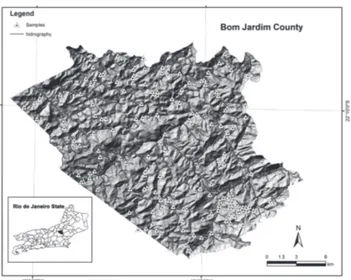
The study area was the municipality of Bom Jardim, RJ, in the mountainous region of the State of Rio de Janeiro (Figure 1). With approximately 390
km2, the area is characterized by the Atlantic
rainforest and high levels of annual rainfall (> 1200 mm/year).
From the geomorphological point of view the area is part of the unit Reverso das Colinas and coast al massive of the high land Serra dos Órgãos, defined by Dantas (2001) as an area with high hills and mountains, interspersed with small areas with a plane relief, below the mountain range (480 - 1,620 m asl). The geological units of the study area,of the central segment of the Ribeira Mobile Belt (Brazilian/Pan-African Orogeny), consist mostly of orthogneisses and migmatites of the Rio Negro complex, granodioritic orthogneisses of the Serra dos Órgãos Batholith interspersed with gneiss bands of the group Paraíba do Sul (leucognaisses and meta sedimentary rocks) and of igneous rocks with gran odioritic to granitic
composition,and more rarely Gabbroic intruded in these units. To a lesser extent, un consolidated alluvial Quaternary deposits occurred with sandy and silty-clayey consistency (Matos et al., 1980; Rio de Janeiro, 1982; Mendes et al., 2007).Due tothe lithological heterogeneity, the regional soil class distribution in the landscape is complex, with higher incidence of Oxisols, Inceptisols and Ultisols, all found in areas of very rugged topography (Calderano Filho et al., 2010).
Soil data
In this study, 208 points were established according to the ease of access and permission of the property owners and sampled between 2009 and 2011 (Figure 1). This soil database (SDB) contains data of 74 full profiles,44 additional profiles and 90 samples of the A horizon, totaling 630 horizons or soil layers. These profiles and samples were harmonized according to the specifications of the global consortium “Global Soil Map.net” (http://www.globalsoilmap.net/). This process consisted of applying the equal-area spline function to establish a new SDB of the properties sand,
silt, clay, organic carbon (OC), and pH(H2O) for layers
that were pre-defined from the original values of the horizons of each soil profile, according to Malone et al. (2009).
The equal-area spline function assumes that the variation in soil properties of a deep soil profile is continuous and the result is the mean value of the soil property analyzed for that depth (Malone et al., 2009). In this way, new data of sand, silt, clay,OC
and pH(H2O) were obtained by this function for
the depths 0-5, 5-15, 15-30, 30-60, 60-100, and 100-200 cm, creating a new SDB. In the specific case of samples of the A horizon, interpolation was extended to a maximum depth of 30 cm, but generally only to a depth of 15 cm. This led to a variation in the number of samples per soil property and layer (Table 1).
All these points were localized by GPS with UTM map projection in zone 23S and Datum Córrego Alegre. The samples were analyzed as described by Embrapa (1997).
Environmental covariates
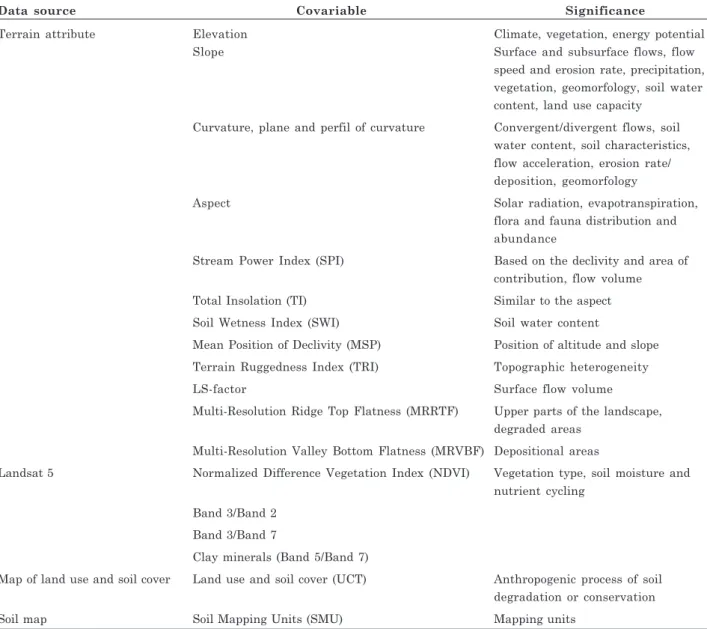
To investigate the prediction of soil properties, environmental covariates with proven correlation with these properties, according to literature data,were selected. Thus, 13 terrain properties derived from a digital elevation model were used with a spatial resolution of 15 m, calculated in SAGAGIS free software, four indices derived from an image of the TM sensor on Landsat 5 September 2011 (calculated in ENVI and resampled to 15 m), and the land use and soil cover obtained from Landsat TM image and the soil distribution in the municipality, reported by Calderano Filho et al. (2010) (Table 2).
Prediction methods
In a first stage of evaluation of the soil properties, the variance in the data of Bom Jardim was compared with that of the database WISE (Batjes, 2008). The relative variance of the data in Bom Jardim was analyzed to contribute to the explanation of the results. Initially, each soil property was assessed to choose the most appropriate method for spatial prediction: MLR, ordinary kriging or co-kriging. For this purpose, the modified procedure of Ciampalini et al. (2012) was applied, in which the prediction method is selected from a decision criterion resulting from an exploratory analysis based on statistical tests. For this analysis, the statistical package R (R Development Core Team, 2013) was used.
This exploratory analysis was performed to answer two questions: what environmental covariate is correlated with the soil property? and does the soil property have a spatial structure? (Ciampalini et al., 2012), according to the decision rule presented in table 3.
For the first question, a classic test of association between paired samples was applied, using Pearson’s correlation coefficient (product moment correlation).
The cor. test function of R was used and the outcome of interest was the probability of the hypothesis of the
absence of a correlation according to the ƿ value for
each paired sample of soil property and of the
environmental covariate. It was assumed that ƿ<0.005
indicated a significant correlation between the paired samples.
To determine whether a soil property has a spatial structure or not, the Mantel test was applied in which
the ƿ value is used to determine the presence or
absence of a correlation between two distance matrices
in R (IDRE, 2012). For this analysis, ƿ<0.10 was
assumed as indicator value of a significant correlation between the two distance matrices (property value and space).
After defining the appropriate prediction method when dealing with kriging or co-kriging, the experimental variograms were adjusted using spherical or exponential models. Ordinary kriging or co-krigingwas applied using the package GSTAT R (Pebesma, 2004).
For the soil properties identified when using MLR as prediction method, in addition to the covariates of terrain properties and Landsat image, we introduced categorical covariates of land use and soil cover (UCT) and soil mapping (SMU) units. This procedure was applied to test the performance of regression with the introduction of UCT and SMU, to assess the importance of including these variables in modeling variables. The MLR model was applied with the
functions lm, update and stepwise of R (R
Development Core Team, 2013), considering the categorical covariates SMU and UCT, in the structure shown in figure 2.
All models in figure 2 were evaluated by the
coefficient of determination (r2) of regression and
cross-validation, aside from analysis of variance (ANOVA) to determine whether the “model” and “reduced model” differed significantly.
RESULTS AND DISCUSSION
The relative values of the variances of soil properties in Bom Jardim(RJ) (Figure 3) were expressed as percentage of the global variance, obtained from the soil database WISE (Batjes, 2008; Gray et al., 2009). Greater variance was noted in
clay and OC than in sand, silt and pH(H2O). In
addition, for pH and OC the variation was greater in the surface (0-30 cm) than in the subsurface layer (30-200 cm). In general, analysis of variance of the data studied compared to the WISE data showed that the variance of the variables analyzed in the study area was small.
The test of correlation showed that only the environmental covariates elevation, aspect, SPI, SWI,
Layer Number of sample
Sand Silt Clay OC pH(H2O) cm
0-5 206 207 208 205 207
5-15 206 207 208 205 207
15-30 134 133 135 132 134
30-60 123 122 124 121 123
60-100 114 113 115 113 116
100-200 105 105 106 105 107
Is there a correlation between paired samples?
Is there a correlation No (> 0.005) Yes (<= 0.005)
No (> 0.10) Mean property value Linear regression
Yes (<= 0.10) Ordinary kriging Co-kriging
between the distance matrices?
Table 3. Decision rules used to select the appropriate model for the prediction of soil properties
Source: Adapted from Ciampalini et al. (2012).
Data source Covariable Significance
Terrain attribute Elevation Climate, vegetation, energy potential
Slope Surface and subsurface flows, flow
speed and erosion rate, precipitation, vegetation, geomorfology, soil water content, land use capacity
Curvature, plane and perfil of curvature Convergent/divergent flows, soil water content, soil characteristics, flow acceleration, erosion rate/ deposition, geomorfology
Aspect Solar radiation, evapotranspiration,
flora and fauna distribution and abundance
Stream Power Index (SPI) Based on the declivity and area of contribution, flow volume
Total Insolation (TI) Similar to the aspect
Soil Wetness Index (SWI) Soil water content
Mean Position of Declivity (MSP) Position of altitude and slope Terrain Ruggedness Index (TRI) Topographic heterogeneity
LS-factor Surface flow volume
Multi-Resolution Ridge Top Flatness (MRRTF) Upper parts of the landscape, degraded areas
Multi-Resolution Valley Bottom Flatness (MRVBF) Depositional areas
Landsat 5 Normalized Difference Vegetation Index (NDVI) Vegetation type, soil moisture and nutrient cycling
Band 3/Band 2 Band 3/Band 7
Clay minerals (Band 5/Band 7)
Map of land use and soil cover Land use and soil cover (UCT) Anthropogenic process of soil degradation or conservation
Soil map Soil Mapping Units (SMU) Mapping units
Table 2. Environmental covariates
MLR with numeral variables
Model 1
Reduced Model
Model 11
UCT Model 2
UCT Reduced Model Model 21
SMU Reduced Model Model 31 SMU
Model 3
Stepwise Update Stepwise
NDVI and b3/b2 resulted in a ƿ value below 0.005, considered a good level of correlation with soil properties in this study (Table 4). Elevation was correlated with the clay content in the 60-100 cm layer, of silt in the 30-60 cm layer, of sand in the 60-100 cm layer, and of OC in the 0-5, 5-15 and 15-30 cm. The covariate SWI was correlated with pH in the 0-5, 5-15 and 15-30 cm layer. The aspect and SPI were only correlated with OC and sand in the 60-100 and 100-200 cm layer, respectively. Environmental covariates derived from the image, NDVI and the relationship between bands b3/b2 were only
significantly correlated (ƿ-value<0.005) with clay in
the 60-100 cm layer.
In similar studies, Padarian et al. (2012) and Aksoy et al. (2012) found a relationship between OC and elevation for soils of Chile and Crete, respectively. Ciampalini et al. (2012) studied soils in northern Tunisia and found a relationship between elevation and slope properties clay, silt and sand. Bodaghabadi et al. (2011) investigated soils in Iran and reported strong correlations between the soil and SWI. Odeh et al. (2007) used the soil wetness index (SWI) for mapping soil properties in Australia and found a good correlation with clay content. For a study area in Ecuador, Lieb et al. (2012) concluded that the main terrain property correlated to soil properties was elevation.
Of the five soil properties analyzed at the six depths, 11 did not correlate with any covariate considered significant and had no spatial structure either (Table 4): silt in the layers 0-5, 5-15, 15-30, 60-100, and 100-200 cm; clay in the 100-200 cm layer; OC in the layers 30-60 and 100-200 cm and
pH(H2O) in the subsurface layers (from 30 to 200
cm). In this case, the mean value of a variable is considered the best basis of estimating or predicting a soil property.
Ordinary kriging was indicated as prediction model for sand and clay in the four surface layers to the depth of 60 cm (Table 4) because there were no significant correlations with the covariates,but
correlations between the spatial distance matrices and the property value. In turn, co-kriging proved most suitable for predicting only three properties: sand in the 100 and 100-200 cm layers, and clay in the 60-100 cm layer (Table 4) due to the correlation of these variables with the covariates and for having a spatial structure in the Mantel test.
The pH(H2O) differed in the correlation with
environmental covariates between the surface (0-30 cm) and subsurface layers (30-200 cm). For the surface layers, the selected prediction method was MLR and the correlation of the covariate SWI was considered significant. The subsurface layers (30-200 cm) were not significantly correlated with any environmental covariate and showed no spatial structure; in these
cases, the mean values of pH(H2O) were considered
the best prediction. The OC had a similar behavior to
that observed for pH(H2O) (Table 4),with significant
correlations for theupper three layers with the covariate elevation, without spatial structure, and selecting MLR as the most appropriate prediction method (Table 4).
The prediction model MLR was selected for silt in the 30-60 cm layer,OC in 0-5, 5-15, 15-30 and
60-100 cm, and pH(H2O) in the surface (0-30 cm)
layers.To these categorical variables the covariates UCT and SMU were added (Figure 2), to check the contribution of these categorical covariates in the estimation performance of the prediction model. The results of MLR associated with the categorical covariates are shown in table 5.
The introduction of the categorical covariates UCT and SMU (Models 2 and 3, respectively) did not
contribute to explain the variation of pH(H2O) in the
topsoil (0-30 cm), whereas the results of the r2 values
of the models 2 and 3 were considered similar to model 1 for these variables (Table 5). This result was probably related to the small variance in data of this property (Figure 3). On the other hand, the introduction of categorical covariates was important to explain the variation in OC in four layers (0-5, 5-15, 15-30 and 60-100 cm), emphasizing the significant
contribution of covariate SMU to raise r2, which
increased from 0.12 to 0.24 in the surface layer (0-5 cm), respectively, for the models 11 and 31. For silt in the layer 30-60 cm, the contribution of covariate
SMU was less significant than that for OC, with r2
ranging from 0.14 in model 11 to 0.18 in model 31 (Table 5).
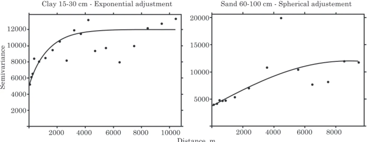
For the soil properties sand and clay (both in the 0-60 cm layers) ordinary kriging was selected as prediction method (Table 4). Co-kriging was the most appropriate method for predicting sand in the layers 60-100 and 100-200 cm and of clay in the 60-100 cm layer. To exemplify the result of applying the models, the properties sand in the 60-100 cm layer (co-kriging) and clay between 15 and 30 cm (ordinary kriging) were selected as predictors for having the best results of coefficient of determination for the methods and in
Figure 3. Variances of soil properties expressed as percentage of the overall variance. Sources: Batjes (2008) and Gray et al. (2009).
40.0
30.0
20.0
10.0
0.0
clay
SOC pH
silt sand 0-30 cm
cross-validation (Table 4). Thus, in order to analyze the spatial trend of these properties, the variograms were constructed and adjusted by exponential and spherical functions (clay in 15-30 cm and sand in the 60-100 cm layer, respectively) (Figure 4). These adjustment functions were used to estimate the value of properties at unsampled locations and thus generate distribution maps of clay and sand in the layers described above.
Comparisons between the observed and estimated OC values in the 15-30 cm layer with MLR, clay in the layer 15-30 cm using ordinary
kriging and sand in the layer 60-100 cm with the use of co-kriging are shown in figure 5. This figure shows the coefficient of determination of MLR for variable CO and of ordinary kriging for clay and
co-kriging for sand, the latter being r2 of cross
validation.
Below we show the spatial distribution maps (Figure 6) for C in the 15-30 cm, clay in the 15-30 cm and sand in the 60-100 cm layer, obtained by MLR, ordinary kriging and co-kriging, respectively.
The percentage distributions of the estimated OC levels in the 15-30 cm, sand in the 60-100 cm and
Layer Correlated covariable(1) Spatial structure(2) Prediction model(3) r2 r2cv(4) cm
Sand
0-5 N o Yes O K 0.37 0.17
5-15 N o Yes O K 0.37 0.16
15-30 N o Yes O K 0.27 0.15
30-60 N o Yes O K 0.17 0.03
60-100 Elevation Yes CK 0.43 0.20
100-200 SPI Yes CK 0.30 0.27
Silt
0-5 N o N o M -
-5-15 N o N o M -
-15-30 N o N o M -
-30-60 Elevation N o MLR 0.14 0.06
60-100 N o N o M -
-100-200 N o N o M -
-Clay
0-5 N o Yes O K 0.21 0.19
5-15 N o Yes O K 0.19 0.19
15-30 N o Yes O K 0.20 0.18
30-60 N o Yes O K 0.13 0.13
60-100 Elevation, NDVI, b3/b2 Yes CK 0.21 0.12
100-200 N o N o M -
-Organic Carbon
0-5 Elevation N o MLR 0.12 0.07
5-15 Elevation N o MLR 0.13 0.07
15-30 Elevation N o MLR 0.20 0.11
30-60 N o N o M -
-60-100 Aspect N o MLR 0.23 0.10
100-200 N o N o M -
-pH(H2O)
0-5 SWI N o MLR 0.12 0.09
5-15 SWI N o MLR 0.12 0.09
15-30 SWI N o MLR 0.10 0.06
30-60 N o N o M -
-60-100 N o N o M -
-100-200 N o N o M -
-Table 4. Results of exploratory analysis based on the selected prediction model
(1) Covariate correlated with
Variable Model(1) r2 Covariable included(2) OC Model1 0.15 All numerical covariables
0-5 cm Model 11 0.12 Elevation + declivity + TRI + MRVBF + b3/b2 Model2 0.19 Elevation + declivity + TRI + MRVBF + b3/b2 * UCT Model 21 0.13 Elevation + MRVBF + b3/b2 * UCT
Model3 0.24 Elevation + declivity + TRI + MRVBF + b3/b2 * SMU
Model 31 0.24 Elevation + declivity + TRI + MRVBF + b3/b2 + SMU + declivity:SMU + TRI:SMU + MRVBF:SMU
OC Model1 0.15 All numerical covariables
5-15 cm Model 11 0.13 Elevation + declivity + aspect + TRI + MRVBF + b5/b7 Model2 0.22 Elevation + declivity + aspect + TRI + MRVBF + b5/b7 * UCT Model 21 0.16 Elevation + aspect + TRI + MRVBF + b5/b7 + UCT
Model3 0.26 Elevation + declivity + aspect + TRI + MRVBF + b5/b7 * SMU
Model 31 0.25 Elevation + declivity + aspect + TRI + MRVBF + b5/b7 + SMU + declivity:SMU + TRI:SMU + MRVBF:SMU
OC Model1 0.24 All numerical covariables
15-30 cm Model 11 0.20 Elevation + aspect + TRI + MRVBF + b3/b2 Model2 0.28 Elevation + aspect + TRI + MRVBF + b3/b2 * UCT Model 21 0.20 Elevation + aspect + TRI + MRVBF + b3/b2 Model3 0.37 Elevation + aspect + TRI + MRVBF + b3/b2 * SMU
Model 31 0.30 Elevation + aspect + TRI + MRVBF + b3/b2 + SMU + elevation:SMU + aspect:SMU + TRI:SMU
OC Model1 0.26 All numerical covariables
60-100 cm Model 11 0.23 Aspect + SWI + factor LS + TRI + NDVI + b3/b7 + b5/b7 Model2 0.44 Aspect + SWI + factor LS + TRI + NDVI + b3/b7 + b5/b7 * UCT
Model 21 0.33 Aspect + SWI + factor LS + TRI + NDVI + b3/b7 + b5/b7 + UCT + aspect:UCT Model3 0.34 Aspect + SWI + fator LS + TRI + NDVI + b3/b7 + b5/b7 * SMU
Model 31 0.32 Aspect + SWI + fator LS + TRI + NDVI + b3/b7 + b5/b7 + SMU + TRI:SMU pH(H2O) Model1 0.16 All numerical covariables
0-5 cm Model 11 0.12 SWI + b3/b7 + b5/b7 Model2 0.17 SWI + b3/b7 + b5/b7 * UCT Model 21 0.12 SWI + b3/b7 + b5/b7 Model3 0.16 SWI + b3/b7 + b5/b7 * SMU Model 31 0.12 SWI + b3/b7 + b5/b7 pH(H2O) Model1 0.15 All numerical covariables 5-15 cm Model 11 0.12 SWI + b3/b7 + b5/b7
Model2 0.16 SWI + b3/b7 + b5/b7 * UCT Model 21 0.12 SWI + b3/b7 + b5/b7 Model3 0.15 SWI + b3/b7 + b5/b7 * SMU Model 31 0.12 SWI + b3/b7 + b5/b7 pH(H2O) Model1 0.15 All numerical covariables 15-30 cm Model 11 0.10 Elevation + SWI + b3/b2
Model2 0.15 Elevation + SWI + b3/b2 * UCT Model 21 0.10 Elevation + SWI + b3/b2 Model3 0.14 Elevation + SWI + b3/b2 * SMU Model 31 0.10 Elevation + SWI + b3/b2 Silt Model1 0.19 All numerical covariables
30-60 cm Model 11 0.14 Curvature + elevation + MSP + MRVBF Model2 0.24 Curvature + elevation + MSP + MRVBF * UCT Model 21 0.14 Curvature + elevation + MSP + MRVBF Model3 0.22 Curvature + elevation + MSP + MRVBF * SMU Model 31 0.18 Curvature + elevation + SMU + curvature:SMU
Table 5. Evaluation results of the MLR models by the introduction of categorical covariates for the functions “update” and “stepwise” of R
clay in the 15-30 cm layer are presented in table 6. According to this framework, a great part of the study area (94 %) has less than 20g/kg C in the 15-30 cm layer, covering an area with a mean elevation of 810 and 752 m, with levels of 0-10 and 10-20 g/kg, respectively. The highest OC levels in this layer are concentrated in the southern part of the area (Figure 6), at amean elevation of 1,225 m. The clay distribution in the15-30 cm layer showed that approximately 75 % of the area contains more than 354g/kg clay, with lowest levels in the southern and southeastern areas (Figure 6). For sand in the 60-100 cm layer, the levels were between 321 and 416 g/kg in 50 % of the study area (Table 6).
Based on our results (Table 4) and considering the layer 0-30 cm as surface layer and 30-200 cm as subsurface layer, according to Gray et al. (2009), a
mean r2 of 0.20 and a mean cross-validation r2 of 0.13
were observed in the surface layer, considering all properties.
Clay and sand in the surface layer estimated by
ordinary kriging showed a mean r2 of 0.27, and mean
r2 cv for cross-validation of 0.17. On the other hand,
for the surface layer of the properties estimated by
MLR [pH(H2O) and OC], the mean r2 of was 0.13 and
mean r2 of cross-validation of 0.08. Although in general
the results of the determination coefficient were considered medium to low, the kriging model performed better than the multiple linear regression (MLR) for the surface layers.
In the subsurface layer the mean values of r2 and
r2 cv were 0.23 and 0.13, respectively, considering all
properties. Ordinary kriging and co-kriging showed mean values for sand and clay of 0.25 and 0.15
(r2 and r2 cv, respectively). The properties of silt from
30-60 cm and of OC from 60-100 cm deep estimated
by MLR showed mean values of 0.19 and 0.08 for r2
and r2 cv, respectively. These results show the same
trend as in the surface layer, where kriging proved to be a better predictor than MLR, although the result
Clay 15-30 cm - Exponential adjustment Sand 60-100 cm - Spherical adjustement
12000
10000
8000
6000
4000
2000
20000
15000
10000
5000
2000 4000 6000 8000 10000 2000 4000 6000 8000
Semivariance
Distance, m
Figure 4.Adjustment of variograms for clay and sand.
r = 0.372
35
30
25
20
15
10
5 10 15 20 25 30 35
200 300 400 500 600
200 300 400 500 600 700
100
OC 15-30 cm - Regression
Observed
Estimulated
Clay 15-30 cm - Ordinary kriging
Sand 60-100 cm - Cokriging 450
400
350
300
250
550
500
450
400
350
300
250
in the surface layer was slightly higher than in the subsurface.
This study explored the potential and limitations of using statistical and geostatistical methods for the
digital mapping of soil properties using a database of soil data, environmental data and available thematic data, according to Ciampalini et al.(2012). The sampling density, an important factor for soil mapping used in different studies (Table 7), shows a wide range of amplitude values, however, most authors used a
density lower than in this study (0.53 samples/km2),
except for Gastaldi et al. (2012), who used a sampling
density of 14 samples/km2 but obtained a lower mean
coefficient of determinationthan for the region of Bom Jardim, RJ, determination.
The ecoregional conditions of the tropical climate in this study differed from the conditions of the studies listed in table 7, which were carried out in temperate climates. The overall analysis of the results discussed in this study showed a trend that, in tropical regions with irregular relief, the higher the sampling density,
the better the results of r2, especially in areas with a
fairly homogenous lithological composition (gneisses, granites and migmatites, mainly). Consequently, the distribution of soil properties varied little. This factor interfered with the models, decreasing the accuracy of the estimates and, for some cases, indicating the use of the mean as the best estimate of certain properties, as observed for 11 of the 30 properties studied (Table 4).
The coefficient of determination (r2) was generally
low to moderate for most of the properties studied, since the better performance can explain 43 % of the variation of the soil property in the case of sand in the 60-100 cm layer, using co-krigingas a prediction model. These results can be considered acceptable, since for quantitative spatial models of soil properties,
r2 values greater than 0.70 are uncommon and in the
literature values below 0.50 are most common (Beckett & Webster, 1971)
The final analysis of the results showed that for the tropical climate conditions in mountainous regions, the digital mapping of soil properties is restricted when the spatial relationships between soil properties, environmental and thematic information are evaluated. This may be partly due to the fact that some soil properties have small variance (silt, pH and sand) as a function of the above-mentioned aspects of geology and local lithologies.
Figure 6. Distribution maps of OC and clay in the 15-30 cm and of sand in the 60-100 cm layer of the study area.
OC 15-30 cm (g/kg)
Clay 15-30 cm (g/kg)
Clay 60-100 cm (g/kg)
OC Clay(1) Sand(1)
15-30 cm 15-30 cm 60-100 cm
g/kg % g/kg % g/kg %
0-10 14.6 219-314 7.3 225-321 12.0 10-20 79.7 314-354 17.3 321-371 21.0 20-40 2.3 354-381 33.6 371-416 29.0 40-100 2.1 381-407 27.5 416-464 25.3 > 100 1.2 407-494 14.3 464-553 12.8
Table 6. Percentage distribution of area for OC, clay and sand
CONCLUSIONS
1.The use of a restricted soil data set in tropical highlands for digital mapping of soil properties correlated with environmental covariates can explain only a small part of the spatial variation of these properties due to the small data variance and the mixture of lithologies with similar composition in the study area.
2. The best performance was obtained with the use of co-kriging for the sand layer at 60-100 cm. In
the mean, the coefficient of determination (r2) was
0.21, considered a low to moderate performance, but common in studies of digital mapping of soil properties. 3. The main factors contributing to the results may be related to the sampling density, the quantity and quality of environmental covariates and the predictive models applied. Further studies with other predictive models, other covariates and more robust soil databases can contribute to the evaluation of digital mapping techniques of soil properties.
LITERATURE CITED
AKSOY, E.; PANAGOS, P. & MONTANARELLA, L. Spatial prediction of soil organic carbon of Crete by using geostatistics. In: MINASNY, B.; MALONE, B.P. &McBRATNEY, A.B., eds. Digital soil assessments and beyond. London, CRC Press, 2012. p.149-154.
BATJES, N.H. ISRIC-WISE Harmonized soil profile dataset (Ver. 3.1). ISRIC - World Soil Information, Wageningen (with dataset). Available at: <http://www.isric.org/isric/Webdocs/ Docs/ISRIC_Report_2008_02.pdf>. Accessed: Jan. 2008. BECKETT, P.H.T. & WEBSTER, R. Soil variability: A review.
Soil Fert., 34:1-15, 1971.
BISHOP, T.F.A. &McBRATNEY, A.B. A comparison of prediction methods for the creation of field-extent soil property maps. Geoderma, 103:149-160, 2001.
BODAGHABADI, M.B.; SALEHI, M.H.; MARTÍNEZ-CASASNOVAS, J.A.; MOHAMMADI, J.; TOOMANIAN, N. & BORUJENI, I.E. Using canonical correspondence analysis (CCA) to identify the most important DEM attributes for digital soil mapping applications. Catena, 86:66-74, 2011.
CALDERANO FILHO, B.; POLIVANOV, H.; GUERRA, A.J.T.; CHAGAS, C.S.; CARVALHO JUNIOR, W. & CALDERANO, S.B. Estudo geoambiental do município de Bom Jardim - RJ, com suporte de geotecnologias: Subsídios ao planejamento de paisagens rurais montanhosas. Soc. Nat., 22:55-73, 2010.
CIAMPALINI, R.; LAGACHERIE, P. & HAMROUNI, H. Documenting GlobalSoilMap.net grid cells from legacy measured soil profile and global available covariates in Northern Tunisia. In: MINASNY, B.; MALONE, B.P. &McBRATNEY, A.B., eds. Digital soil assessments and beyond. London, CRC Press, 2012. p.439-444.
DANTAS, M.E. Geomorfologia do Estado do Rio de Janeiro. In: COMPANHIA DE PESQUISA DE RECURSOS MINERAIS - CPRM. Serviço Geológico do Brasil. Estudo geoambiental do Estado do Rio de Janeiro. Rio de Janeiro, CPRM/Embrapa Solos; Niterói, DRM-RJ, 2001. CD-ROM EMPRESA BRASILEIRA DE PESQUISA AGROPECUÁRIA -EMBRAPA. Centro Nacional de Pesquisa de Solos. Manual de métodos de análise de solo. 2.ed. Rio de Janeiro, 1997. 212p. (Série Documentos, 1)
ERSAHIN, S. Comparing ordinary kriging and cokriging to estimate infiltration rate. Soil Sci. Soc. Am. J., 67:1848-1855, 2003.
GASTALDI, G.; MINASNY, B. &McBRATNEY, A.B. Mapping the occurrence and thickness of soil horizons within soil profiles. In: MINASNY, B.; MALONE, B.P. & McBRATNEY, A.B., eds. Digital soil assessments and beyond. London, CRC Press, 2012. p.145-148.
GOOVAERTS, P. Geostatistics in soil science: State-of-the-art and perspectives. Geoderma, 89:1-45, 1999.
GRAY, J.M.; HUMPHREYS, G.S. & DECKERS, J.A. Relationships in soil distribution as revealed by a global soil database. Geoderma, 150:309-323, 2009.
GRUNWALD, S.; OSBORNE, T.Z. & REDDY, K.R. Temporal trajectories of phosphorus and pedo-patterns mapped in Water Conservation Area 2, Everglades, Florida, USA.Geoderma, 146:1-13, 2008.
HENGL, T.; TOORMANIAN, N.; REUTER, H.I. & MALAKOUTI, M.J. Methods to interpolate soil categorical variables from profile observations: lessons from Iran. Geoderma, 140:417-427, 2007.
INSTITUTE FOR DIGITAL RESEARCH AND EDUCATION -IDRE. Statistical Consulting Group.Introduction to SAS. Available at: <http://www.ats.ucla.edu/stat/sas/notes2>. Accessed: Nov. 2012.
Source Number of sample Area Density Mean r2
km2 no. of sample/km2
In this study 208 390 0.530 0.21
Aksoy et al. (2012) 97 8336 0.012 0.51 a 0.56
Gastaldi et al. (2012) 1050 75 14 0.18
Malone et al. (2009) 341 1500 0.280 0.44
Gray et al. (2009) 1646 Global scale - 0.29
Ciampalini et al. (2012) 89 2822 0.032
JENKS, G.F. & CASPALL, F.C. Error on choroplethic maps: Definition, measurement, reduction. An. Assoc. Am. Geogr., 61:217-244, 1971.
LAGACHERIE, P. & McBRATNEY, A.B. Spatial soil information systems and spatial soil inference systems: perspectives for digital soil mapping. In: LAGACHERIE, P.; McBRATNEY, A.B. & VOLTZ, M., eds. Digital soil mapping: An introductory perspective. Amsterdam, Elsevier, 2007. p.3-22. (Developments in Soil Science, 31) LIEB, M.; GLASER, B. & HUWE, B. Uncertainty in the spatial prediction of soil texture Comparison of regression tree and random forest models. Geoderma, 170:70-79, 2012. MABIT, L.; BERNARD, C.; MAKHLOUF, M. & LAVERDIÈRE,
M.R. Spatial variability of erosion and soil organic matter content estimated from 137Cs measurements and geostatistics. Geoderma, 145:245-251, 2008.
MALONE, B.P.; McBRATNEY, A.B.; MINASNY, B. & LASLETT, G.M. Mapping continuous depth functions of soil carbon storage and available water capacity. Geoderma, 154:138-152, 2009.
MATOS, G.; FERRARI, P. & CAVALCANTI, J. Projeto Faixa Calcária Cordeiro - Cantagalo. Belo Horizonte, DNPM/ CPRM, 1980.
McBRATNEY, A.B.; ODEH, I.O.A.; BISHOP, T.F.A.; DUNBAR, M.S. & SHATAR, T.M. An overview of pedometric techniques for use in soil survey. Geoderma, 97:293-327, 2000.
McBRATNEY, A.B.; SANTOS, M.L.M. & MINASNY, B. On digital soil mapping. Geoderma, 117:3-52, 2003.
MENDES, J.C.; TEIXEIRA, P.A.D.; MATOS, G.C.; LUDKA, I.P.; MEDEIROS, F.F. & ÁVILA, C.A. Geoquímica e geocronologia do granitoide Barra Alegre, faixa móvel Ribeira, Rio de Janeiro. R. Bras. Geoci., 37:101-113, 2007.
MINASNY, B. & HARTEMINK, A.E. Predicting soil properties in the tropics. Earth Sci. Rev., 106:52-62, 2011.
ODEH, I.O.A.; CRAWFORD, M. & McBRATNEY, A.B. Digital mapping of soil attributes for regional and catchment modelling, using ancillary covariates, statistical and geostatistical techniques. In: LAGACHERIE, P.; McBRATNEY, A.B. & VOLTZ, M., eds. Digital soil mapping: An introductory perspective. Amsterdam, Elsevier, 2007. p.437-453. (Developments in Soil Science, 31)
PADARIAN, J.; PÉREZ-QUEZADA, J. & SEGUEL, O. Modelling the distribution of organic carbon in the soils of Chile. In: MINASNY, B.; MALONE, B.P. & McBRATNEY, A.B., eds. Digital soil assessments and beyond. London, CRC Press, 2012. p.329-333.
PEBESMA, E.J. Multivariable geostatistics in S: The GSTAT package. Comput. Geosci., 30:683-691, 2004.
R DEVELOPMENT CORE TEAM. R: A language and environment for statistical computing, R Foundation for Statistical Computing, Vienna, 2013. Available at: <http://www.r-project.org/isbn 3- 900051-07-0>. Accessed: May 2013. RIO DE JANEIRO. Secretaria de Estado de Indústria,
Comércio e Turismo. Departamento de Recursos Minerais. DRM. Projeto Carta Geológica do Estado do Rio de Janeiro. Folhas: Duas Barras e Trajano de Morais. 1982. RIVERO, R.G.; GRUNWALD, S. & BRULAND, G.L.
Incorporation of spectral data into multivariate geostatistical models to map soil phosphorus variability in a Florida wetland. Geoderma, 140:428-443, 2007. SUN, W.; MINASNY, B. & McBRATNEY, A.B. Analysis and
prediction of soil properties using local regression-kriging.Geoderma, 171-172:16-23, 2012.