* Corresponding author:
E-mail: [email protected]
Received: January 21, 2017
Approved: August 28, 2017
How to cite: Moraes AGL, Francelino MR, Carvalho Júnior W, Pereira MG, Thomazini A, Schaefer CEGR. Environmental correlation and spatial
autocorrelation of soil properties in Keller Peninsula, Maritime Antarctica. Rev Bras Cienc Solo. 2017;41:e0170021.
https://doi.org/10.1590/18069657rbcs20170021
Copyright: This is an open-access article distributed under the terms of the Creative Commons Attribution License, which permits unrestricted use, distribution, and reproduction in any medium, provided that the original author and source are credited.
Division - Soil in Space and Time | Commission - Pedometry
Environmental Correlation and
Spatial Autocorrelation of Soil
Properties in Keller Peninsula,
Maritime Antarctica
André Geraldo de Lima Moraes(1)
, Marcio Rocha Francelino(2)
, Waldir de Carvalho Junior(3)
, Marcos Gervasio Pereira(4)
, André Thomazini(5)* and Carlos Ernesto Gonçalves
Reynaud Schaefer(6)
(1)
Universidade Federal Rural do Rio de Janeiro, Departamento de Solos, Programa de Pós-Graduação em Agronomia - Ciência do Solo, Seropédica, Rio de Janeiro, Brasil.
(2)
Universidade Federal Rural do Rio de Janeiro, Departamento de Solos, Seropédica, Rio de Janeiro, Brasil. (3)
Empresa Brasileira de Pesquisa Agropecuária, Embrapa Solos, Rio de Janeiro, Rio de Janeiro, Brasil. (4)
Universidade Federal Rural do Rio de Janeiro, Departamento de Solos, Seropédica, Rio de Janeiro, Brasil. (5)
Universidade Federal de Viçosa, Departamento de Solos, Programa de Pós-Graduação em Solos e Nutrição de Plantas, Viçosa, Minas Gerais, Brasil.
(6)
Universidade Federal de Viçosa, Departamento de Solos, Viçosa, Minas Gerais, Brasil.
ABSTRACT: The pattern of variation in soil and landform properties in relation to environmental covariates are closely related to soil type distribution. The aim of this study was to apply digital soil mapping techniques to analysis of the pattern of soil property variation in relation to environmental covariates under periglacial conditions at Keller Peninsula, Maritime Antarctica. We considered the hypothesis that covariates normally used for environmental correlation elsewhere can be adequately employed in periglacial areas in Maritime Antarctica. For that purpose, 138 soil samples from 47 soil sites were collected for analysis of soil chemical and physical properties. We tested the correlation between soil properties (clay, potassium, sand, organic carbon, and pH) and environmental covariates. The environmental covariates selected were correlated with soil properties according to the terrain attributes of the digital elevation model (DEM). The models evaluated were linear regression, ordinary kriging, and regression kriging. The best performance was obtained using normalized height as a covariate, with an R2 of
0.59 for sand. In contrast, the lowest R2 of 0.15 was obtained for organic carbon, also using
the regression kriging method. Overall, results indicate that, despite the predominant periglacial conditions, the environmental covariates normally used for digital terrain mapping of soil properties worldwide can be successfully employed for understanding the main variations in soil properties and soil-forming factors in this region.
INTRODUCTION
Antarctica, which is the coldest continent, has unique climatic and weathering conditions that lead to unique soil formation in ice-free areas at very slow rates (Simas et al., 2008). Pedogenesis in Antarctica is generally less advanced, due to the combination of freezing conditions, low liquid water availability, weak biological activity, and chemical and physical processes occurring only during the summer. In comparison with continental Antarctica, the Maritime region has higher temperature and precipitation rates, contributing to greater colonization of plant species and soil microorganisms, which favors a higher degree of weathering (Pereira and Putzke, 2013). In addition, these factors are frequently associated with terrestrial input of nutrients by marine birds (guano), which are highly important for soil-forming processes in Antarctica, enhancing pedogenesis through the phosphatization process and forming widespread ornithogenic soils (Simas et al., 2008).
Ornithogenic soils are characterized by low pH, deep soil development, and very high phosphorus contents (Mehlich-1), and total organic carbon contents (Simas et al., 2008). In addition, soil types and properties vary significantly across the landscape, mainly related to landscape characteristics, especially drainage (Pereira and Putzke, 2013). Antarctic soils have been the subject of several studies (Beyer et al., 2000; Simas et al., 2008; Francelino et al., 2011; Moura et al., 2012) that have promoted an increasing understanding of soil-forming processes and soil distribution and classification.
The foundations of the Digital Soil Mapping (DSM) technique were laid by McBratney et al. (2003). Lagacherie and McBratney (2006) defined DSM as “the creation of spatial information systems of soils by numerical models in order to infer the spatial and temporal variations of soil properties and classes, from observations, knowledge and covariate-related environmental data”. Recently, DSM has improved soil studies and has been tested and used in soil surveys around the world (Carvalho Junior et al., 2014; Hartemink and Minasny, 2014; Vaysse and Lagacherie, 2015; Chagas et al., 2016; Pahlavan-Rad et al., 2016; Malone et al., 2017). However, little is known about the use of digital soil and environmental mapping techniques in the Antarctic environment.
The DSM has emerged as an alternative to resolve uncertainties and subjectivities that the traditional approach presents. In this context, new methods for quantitative modeling of soil distribution have been proposed to describe, classify, and study the patterns of spatial variation of soils across the landscape. From this, it has been possible to increase knowledge of spatial variability of soils across the landscape, generating accurate information about this natural resource. This has been accomplished through a set of quantitative techniques called Pedometrics (Hartemink and Minasny, 2014). This technique becomes important and useful in regions where detailed soil sampling and description is highly complex and difficult due to the local characteristics, such as Antarctica.
The aim of this study was to apply digital soil mapping techniques to analyze the pattern of variation of soil properties in relation to environmental covariates under periglacial conditions at Keller Peninsula, Maritime Antarctica. We tested the hypothesis that covariates normally used for environmental correlation worldwide (Hartemink and Minasny, 2014) can be adequately employed in periglacial areas of Maritime Antarctica to understand spatial distribution of soil processes/properties. These are possibly some of the most complex and anisotropic areas for soil mapping purposes, due to their natural heterogeneity on short-range scales.
MATERIALS AND METHODS
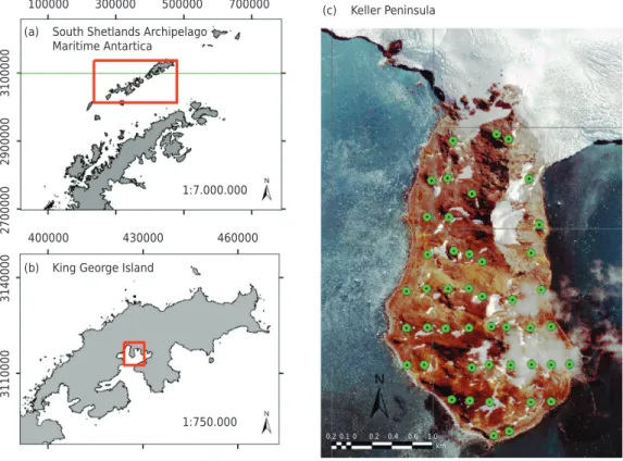
Study area
(Figure 1). The monthly mean air temperature ranges from -6.4 °C in July to +2.3 °C in February, and the mean annual precipitation is 367 mm (INPE, 2009). The altitude ranges from 0 to 340 m a.s.l. (Francelino et al., 2011). The geology is predominantly basalt-andesites and pyritized andesite rocks. Overall, soils are usually shallow and skeletal, mainly composed of Leptosols and Cryosols (Francelino et al., 2011).
Soil sampling
Soil samples were collected in a grid arrangement in February 2012, covering most of the ice-free area of the peninsula, from a total of 47 points at the depths of 0.00-0.05, 0.05-0.10, and 0.10-0.30 m. We used a semi-regular grid with a minimum separation distance of 180 m and maximum separation distance of 500 m between neighboring points. All collection points were marked with a geodetic GPS device (high accuracy ± 10 mm error), CS Leica 1200 + model (Figure 1).
Soil analyses
The soil samples were air dried, ground, and passed through a 2-mm sieve to remove larger pieces of root material, pebbles, and gravels. Particle size analysis was performed by the pipette method (Claessen, 1997). The pH was determined in a 1:5 soil:deionized water ratio. Exchangeable potassium was extracted with Melich-1 and determined by flame emission (Claessen, 1997). Total soil organic carbon was quantified by wet oxidation with 0.167 mol L-1 K
2Cr2O7 in the
presence of sulfuric acid with external heating (Yeomans and Bremner, 1988).
Geostatistical model
Environmental covariates were derived from a digital elevation model (DEM) with a spatial resolution of 5 m (adapted from Mendes Junior, 2012). These covariates were calculated using the System for Automated Geoscientific Analyses (SAGA GIS) and ArcGIS 10.0 software. The terrain characteristics used were aspect, curvature, plan curvature,
100000
South Shetlands Archipelago Maritime Antartica
(a)
King George Island (b)
Keller Peninsula (c)
2700000
2900000
3100000
3110000
3140000
300000 500000 700000
400000 430000 460000
1:750.000
Projection UTM - Zone 21S - Datum WGS 84 1:7.000.000
0.2 0.1 0 0.2 0.4 0.6 1.0 km
Figure 1. Localization of the study area (a, b) and the collection points in the soil grid in Keller
profile curvature, slope, LS-Factor, terrain roughness index (TRI), topographic wetness index, multiresolution index of valley bottom flatness (MrVBF), multiresolution ridge top flatness (MrRTF), normalized height, catchment area, slope height, standardized height, and potential incoming solar radiation (total, direct, and diffuse). The covariate values were extracted from thematic maps (raster), which were converted to a vectorial theme so that the entire surface of the peninsula was covered.
Three candidates of geostatistical model functions were evaluated for all depths: linear regression (R), ordinary kriging (OK), and regression kriging (RK). The correlations between environmental covariates and soil properties were assessed using Pearson’s product-moment correlation coefficient, in order to verify which covariate is correlated with the soil property (Carvalho Junior et al., 2014). Correlation analyses were performed with the R software package, using the cor.test command, testing the association between paired samples (R Development Core Team, 2007). In this case, through p-values, we determined if the correlation is acceptable or not. The p-values ranging from 0.005 to 0.05 were considered most restrictive and least restrictive, respectively.
We also applied the Mantel test to check the spatial dependence structure of the variables. This test indicates the possibility of using geostatistics for spatialization of a given soil property. The p-value resulting from the Mantel Test was also considered as a decision parameter, in which values greater than 0.10 indicate spatial dependence (Carvalho Junior et al., 2014). Thus, analyzing the results together with the initial assessment, cor.test, and Mantel test, the best way to model the distribution of variables was decided depending on the covariates, as verified by Ciampalini et al. (2012). After defining the appropriate prediction method, the experimental variograms were developed using spherical, exponential, and Gaussian models. Modeling was performed using the GSTAT R package (R Development Core Team, 2007).
After that, for spatialization of the properties modeled, all points containing the values obtained were converted to raster format from the DEM as a spatial reference. In this process, we disregarded areas of glaciers, lakes, and rock outcrops were defined as ice-free areas [features were extracted from the map generated by Francelino et al. (2011)]. Performance of the models was tested based on k-fold cross-validation (k = 10) and the coefficient of determination of the models from the linear regression (Kvålseth, 1985).
RESULTS AND DISCUSSION
Preliminary analysis indicated soil variables and their respective depths were best correlated with the environmental covariates considered, as well as the most appropriate method to achieve soil properties spatialization (Table 1). Only the R2 values were
considered, whereas values derived from cross-validation were discarded, only being used to select the best model. The regression method was the most recommended, indicating high correlation between the variables and the covariates. This can also be explained by the large distance of separation between observations, reducing identification of the spatial autocorrelation structure. When a given variable exhibited spatial dependence, regression-kriging or ordinary kriging was used as a prediction method.
Table 1. Decision rules for selecting the appropriate DSM function [adapted from Ciampalini et al. (2012)]
Variate Depth Covariates Method
m
Clay 0.00-0.05 Plan curvature + TWI R
Sand 0.10-0.30 Normalized height RK
Potassium 0.05-0.10 Slope + LS-factor + catchment area + MrRTF+ TRI R pH 0.05-0.10 Plan curvature + Direct insolation + Total insolation R
Organic carbon 0.00-0.05 None OK
TWI: topographic wetness index; TRI: terrain ruggedness index; R: regression; OK: ordinary kriging; RK:
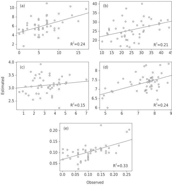
Clay contents were best modeled by a regression method, achieving an R² of 0.24 (Table 1). Generally, clay contents in soils from Keller Peninsula are very low, with a maximum value around 100 g kg-1, and an average of 45 g kg-1 (standard deviation = 2.17 g kg-1).
The model that showed the best result took the “plan curvature” and “topographic wetness index” (TWI) of the covariates into account (Figure 2a). The low clay contents and the high heterogeneity of this soil property certainly affected the low R² parameter. In addition, the lack of spatial structure is strongly related to the large separation among observation points, and spatial dependence cannot be properly identified.
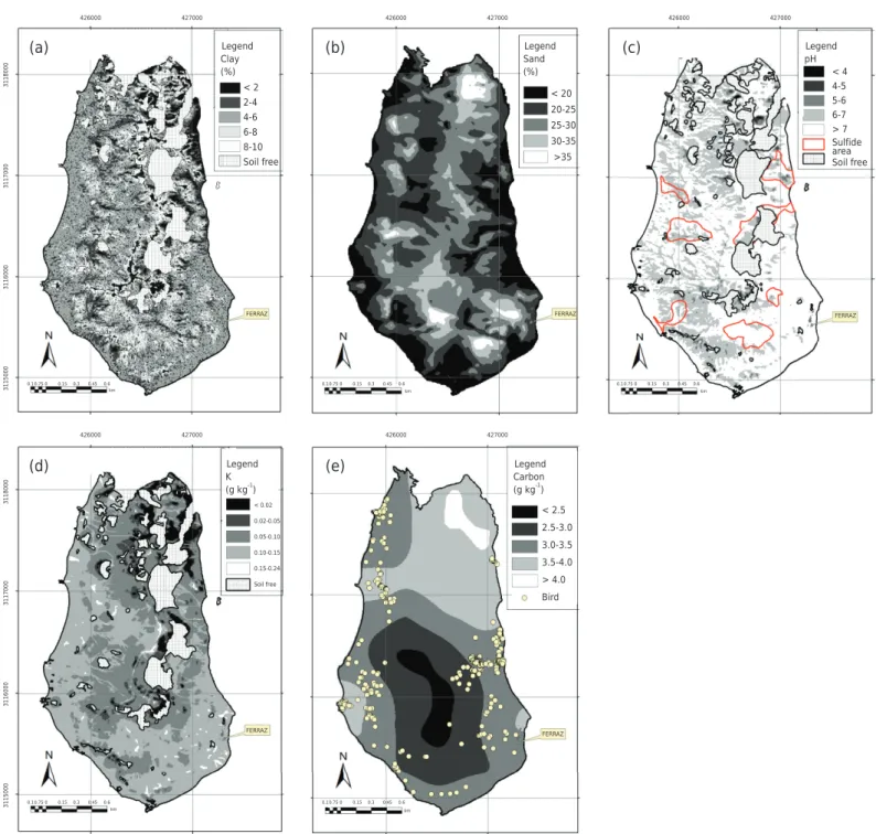
Spatialization of the clay property by the proposed model (Figure 3) showed lower values in the areas of ridges, cliffs, and rocky outcrops, which is expected for their low degree of weathering (Simas et al., 2008; Francelino et al., 2011). Conversely, the highest values are found in flat areas free of rock outcrops at the top of the landscape, such as the Tyrrel plateau and areas to the south of the peninsula, all influenced by sulfide-rich andesite (Francelino et al., 2011). This is consistent with an advanced degree of weathering in these sulfate-rich soils, as observed by Simas et al. (2008) and Souza et al. (2012) in the same peninsula. Both studies revealed the presence of minerals such as natrojarosite and jarosite and low-crystalline iron-oxide abundance in the clay fraction, following sulfide oxidation and sulfate soil formation.
Figure 2. Relation between the estimated and observed values of clay (a), sand (b), pH (c),
potassium (d), and soil organic carbon (e).
2 4 6 8 10
0 5 10 15
20 25 30 35 40
10 15 20 25 30 35 40 45
6 6.5 7 7.5 8
5 6 7 8 9
2.5 3.0 3.5 4.0
1 2 3 4 5 6 7
0.05 0.10 0.15 0.20
0.0 0.05 0.10 0.15 0.20 R2
=0.33
0.25
Estimate
d
Observed
(a) (b)
(c)
(e)
(d) R2
=0.24
R2
=0.15
R2=0.21
R2
The model chosen by regression considered the environmental covariates of plan curvature and solar radiation, with an R2 value of 0.24 (Figure 2d). Sulaeman et al. (2012) studied the
distribution of soil pH, reporting that the covariate that showed the best correlation with pH was the multiresolution ridge top flatness (MrRTF), along with elevation, with an R2 of 0.38.
Several factors may be influencing the ionic concentration and pH of the soil solution in Keller Peninsula. According to Souza et al. (2012) and Simas et al. (2008), the presence of sulfates derived from sulfide oxidation is always associated with greater soil acidity. Although the geology was not considered as a covariate in this analysis, the result of the model suggests the influence of parent material on the spatialization of this property, since sulfate-affected soils coincide with areas of low pH (Figure 4) (Francelino et al., 2011). Overall, a trend of higher pH at the western side of the peninsula compared to the eastern side was observed, according to the thematic maps. This pattern was also observed by Souza et al. (2012). The distribution of exchangeable K considered five covariates and a linear regression model, with an R2 of 0.33 (Figure 2e). The distribution of exchangeable K levels showed an altitudinal
gradient, with higher levels in the lower parts of the landscape, especially in depositional features and scree slopes, and not only along the coastal areas. Hence, it did not follow the same trend as Na (Figure 4). This result can be attributed to the combination of saline sprays, with a lateral redistribution by K-rich leachates from upland sources (Simas et al., 2008).
The soil organic carbon (SOC) in Keller Peninsula showed a spatial dependence structure, which was spatialized by the ordinary kriging method, exhibiting the lowest R2 (0.15)
(Table 2, Figures 2f and 3c). Soil organic carbon showed a greater range value than the other soil properties (946.90 m). Goodman et al. (2012) studied the spatial distribution of soil organic carbon in a former glacial area in central Indiana (USA) and found a correlation between TWI and soil carbon, with an R2 of 0.33. This indicates the intrinsic
difficulty of predicting SOC amounts based on a few environmental covariates.
The primary input of SOC in Keller Peninsula is guano produced by birds and decomposition of the few plants that grow on soils (Thomazini et al., 2016). The plant communities formed
Figure 3. Semivariograms fitted to sand (a) and soil organic carbon contents (b).
20 40 60 80 100 120
0 500 1000 1500 2000 2500
0.5 1.0
Distance (m) 1.5
500 1000 1500
Semivarianc
e
(a)
by Deschampsia Antarctica and Colobanthus quitensis and mixed lichen and mosses are very common in areas close to bird nests (Victoria et al., 2013). They are always associated with increasing SOC (Figure 4). In addition, higher plateaus under a dense Usnea sp. coverage (lichen) also increased the amount of SOC; the greatest content in the northern peninsula were at points with dense fields of Usnea sp.
Table 2. Model type and parameters of the semivariograms developed for the soil properties studied in Keller Peninsula
Property Model R2 R2 CV(1) Adjust Psill Range Nugget
Sand Regression Kriging 0.21 0.19 Gaussian 39.160 155.417 16.212
Organic carbon Ordinary Kriging 0.15 0.04 Spherical 0.491 946.903 1.106
(1)
Cross validation.
Figure 4. Thematic maps of clay (a), sand (b), pH (c), potassium (d), and soil organic carbon (e) estimated in Keller Peninsula.
(a) Legend
Clay (%)
< 2 2-4 4-6 6-8 8-10 Soil free
Legend Sand (%)
< 20 20-25 25-30 30-35 >35
Legend K (g kg-1)
< 0.02
0.02-0.05
0.05-0.10
0.10-0.15
0.15-0.24
Soil free
Legend Carbon (g kg-1)
< 2.5 2.5-3.0 3.0-3.5 3.5-4.0 > 4.0 Bird
Legend pH
< 4 4-5 5-6 6-7
Sulfide area > 7
Soil free
FERRAZ
3115000
3116000
3117000
3118000
426000 427000 426000 427000
3115000
3116000
3117000
3118000
426000 427000 426000 427000
426000 427000
FERRAZ FERRAZ
FERRAZ FERRAZ
(b)
(d) (e)
(c)
0.1 0.75 0 0.15 0.3 0.45 0.6 km
0.1 0.75 0 0.15 0.3 0.45 0.6
0.1 0.75 0 0.15 0.3 0.45 0.6 0.1 0.75 0 0.15 0.3 0.45 0.6
0.1 0.75 0 0.15 0.3 0.45 0.6
km km
CONCLUSIONS
The environmental covariates traditionally used for digital terrain mapping in other regions can be successfully applied to estimate the variation in soil properties in Maritime Antarctica. Soil organic carbon proved to be spatially well-structured, with a high range of values. However, the opposite was observed for sand. The values of pH are linked with the occurrence of sulfate zones, which reduced pH values. Furthermore, sodium contents were closely related to salt sprays in coastal areas, with no strong spatial relationship with potassium distribution in the peninsula. The large separation between observation points reduces identification of the spatial autocorrelation structure, indicating that the sampling arrangement was not suitable for properly identifying spatial dependence. Hence, to best capture spatial dependence, a more detailed grid with lower separation between neighboring points is needed. Environmental covariates are useful for a better understanding of soil distribution, allowing inferences to be made regarding properties with environmental significance for monitoring landscape changes. It is necessary to use different statistical methods, regarding the spatial characteristics of each property in relation to environmental covariates, in which models are tailored to each specific environment.
ACKNOWLEDGMENTS
We thank the Brazilian National Research and Technology Council (CNPq) for funding this study, the Brazilian Antarctic Program, and the Comandante Ferraz Brazilian Antarctic Station for logistical assistance during summer 2012. This study is a contribution of the Terrantar Centre (INCT Criosfera), with joint funding from the CNPq. Professor Carlos Schaefer thanks CAPES for granting a sabbatical leave at SPRI-Cambridge.
REFERENCES
Beyer L. Properties, formation, and geo-ecological significance of organic soils in the coastal region of
East Antarctica (Wilkes Land). Catena. 2000;39:79-93. https://doi.org/10.1016/S0341-8162(99)00090-9
Carvalho Junior W, Lagacherie P, Chagas CS, Calderano Filho B, Bhering SB. A regional-scale assessment of digital mapping of soil attributes in a tropical hillslope environment. Geoderma. 2014;232-234:479-86. https://doi.org/10.1016/j.geoderma.2014.06.007
Chagas CS, Carvalho Junior W, Bhering SB, Calderano Filho B. Spatial prediction of soil surface texture in a semiarid region using random forest and multiple linear regressions. Catena. 2016;139:232-40. https://doi.org/10.1016/j.catena.2016.01.001
Ciampalini R, Lagacherie P, Hamrouni H. Documenting globalsoilmap.net grid cells from legacy
measured soil profile and global available covariates in Northern Tunisia. In: Minasny B, Malone
BP, McBratney AB. Digital soil assessments and beyond. Boca Raton: CRC Press; 2012. p.437-44.
Claessen MEC, organizador. Manual de métodos de análise de solo. 2.ed. Rio de Janeiro: Embrapa Solos; 1997.
Francelino MR, Schaefer CEGR, Simas FNB, Fernandes Filho EI, Souza JJLL, Costa LM. Geomorphology and soils distribution under paraglacial conditions in an ice-free area of Admiralty Bay, King George Island, Antarctica. Catena. 2011;85:194-204. https://doi.org/10.1016/j.catena.2010.12.007
Goodman JM, Owens PR, Libohova Z. Predicting soil organic carbon using mixed conceptual and geostatistical models. In: Minasny B, Malone BP, McBratney AB. Digital soil assessments and beyond. Boca Raton: CRC Press; 2012. p.155-9.
Hartemink AE, Minasny B. Towards digital soil morphometrics. Geoderma. 2014;230-231:305-17. https://doi.org/10.1016/j.geoderma.2014.03.008
Instituto Nacional de Pesquisas Espaciais - INPE. Centro de previsão de tempo e estudos climáticos; 2009 [acesso em 10 Jul 2010]. Disponível em: http://antartica.cptec.inpe.br
Kvålseth TO. Cautionary note about R2
Lagacherie P, McBratney AB. Spatial soil information systems and spatial soil inference systems: perspectives for digital soil mapping. Dev Soil Sci. 2006;31:3-22. https://doi.org/10.1016/S0166-2481(06)31001-X
Malone BP, Styc Q, Minasny B, McBratney AB. Digital soil mapping of soil carbon at the farm scale: a spatial downscaling approach in consideration of measured and uncertain data. Geoderma. 2017;290:91-9. https://doi.org/10.1016/j.geoderma.2016.12.008
McBratney AB, Santos MLM, Minasny B. On digital soil mapping. Geoderma. 2003;117:3-52. https://doi.org/10.1016/S0016-7061(03)00223-4
Mendes Junior CW, Dani N, Arigony-Neto J, Simões JC, Velho LF, Ribeiro RR, Parnow I, Bremer UF, Fonseca Júnior ES, Erwes HJB. A new topographic map for Keller Peninsula, King George Island. Pesq Antart Bras. 2012;5:105-13.
Moura PA, Francelino MR, Schaefer CEGR, Simas FNB, Mendonça BAF. Distribution and characterization of soils and landform relationships in Byers Peninsula, Livingston Island, Maritime Antarctica. Geomorphology. 2012;155-156:45-54. https://doi.org/10.1016/j.geomorph.2011.12.011
Pahlavan-Rad MR, Khormali F, Toomanian N, Brungard CW, Kiani F, Komaki CB, Bogaert P. Legacy soil maps as a covariate in digital soil mapping: a case study from Northern Iran. Geoderma. 2016;279:141-8. https://doi.org/10.1016/j.geoderma.2016.05.014
Pereira AB, Putzke J. The Brazilian research contribution to knowledge of the plant communities from Antarctic ice free areas. An Acad Bras Cienc. 2013;85:923-35. https://doi.org/10.1590/S0001-37652013000300008
R Development Core Team. R: a language and environment for statistical computing. Vienna, Austria: R Foundation for Statistical Computing; 2007. Available at: http://www.R-project.org.
Simas FNB, Schaefer CEGR, Albuquerque Filho MR, Francelino MR, Fernandes Filho EI, Costa
LM. Genesis, properties and classification of Cryosols from Admiralty Bay, maritime Antarctica.
Geoderma. 2008;144:116-22. https://doi.org/10.1016/j.geoderma.2007.10.019
Souza JJLL, Schaefer CEGR, Abrahão WAP, Mello JWV, Simas FNB, Silva J, Francelino MR.
Hydrogeochemistry of sulfate-affected landscapes in Keller Peninsula, Maritime Antarctica.
Geomorphology. 2012;155-156:55-61. https://doi.org/10.1016/j.geomorph.2011.12.017
Sulaeman Y, Sarwani M, Minasny B, McBratney AB, Sutandi A, Barus B. Soil-landscape models to predict soil pH variation in the Subang Region of West Java, Indonesia. In: Minasny B, Malone BP, McBratney AB. Digital soil assessments and beyond. Boca Raton: CRC Press; 2012. p.317-23.
Thomazini A, Francelino MR, Pereira AB, Schünemann AL, Mendonça ES, Almeida PHA, Schaefer CEGR. Geospatial variability of soil CO2-C exchange in the main terrestrial ecosystems of Keller Peninsula, Maritime Antarctica. Sci Total Environ. 2016;562:802-11. https://doi.org/10.1016/j.scitotenv.2016.04.043
Vaysse K, Lagacherie P. Evaluating digital soil mapping approaches for mapping GlobalSoilMap soil properties from legacy data in Languedoc-Roussillon (France). Geoderma Regional. 2015;4:20-30. https://doi.org/10.1016/j.geodrs.2014.11.003
Victoria FC, Albuquerque MP, Pereira AB, Simas FNB, Spielmann AA, Schaefer CEGR.
Characterization and mapping of plant communities at Hennequin Point, King George Island, Antarctica. Polar Res. 2013;32:19261. https://doi.org/10.3402/polar.v32i0.19261