COMPARISON BETWEEN ARTIFICIAL NEURAL NETWORKS
AND MAXIMUM LIKELIHOOD CLASSIFICATION IN DIGITAL
SOIL MAPPING
(1)César da Silva Chagas(2), Carlos Antônio Oliveira Vieira(3) & Elpídio Inácio Fernandes Filho(4)
SUMMARY
Soil surveys are the main source of spatial information on soils and have a range of different applications, mainly in agriculture. The continuity of this activity has however been severely compromised, mainly due to a lack of governmental funding. The purpose of this study was to evaluate the feasibility of two different classifiers (artificial neural networks and a maximum likelihood algorithm) in the prediction of soil classes in the northwest of the state of Rio de Janeiro. Terrain attributes such as elevation, slope, aspect, plan curvature and compound topographic index (CTI) and indices of clay minerals, iron oxide and Normalized Difference Vegetation Index (NDVI), derived from Landsat 7 ETM+ sensor imagery, were used as discriminating variables. The two classifiers were trained and validated for each soil class using 300 and 150 samples respectively, representing the characteristics of these classes in terms of the discriminating variables. According to the statistical tests, the accuracy of the classifier based on artificial neural networks (ANNs) was greater than of the classic Maximum Likelihood Classifier (MLC). Comparing the results with 126 points of reference showed that the resulting ANN map (73.81 %) was superior to the MLC map (57.94 %). The main errors when using the two classifiers were caused by: a) the geological heterogeneity of the area coupled with problems related to the geological map; b) the depth of lithic contact and/or rock exposure, and c) problems with the environmental correlation model used due to the polygenetic nature of the soils. This study confirms that the use of terrain attributes together with remote sensing data by an ANN approach can be a tool to facilitate soil mapping in Brazil, primarily due to the availability of low-cost remote sensing data and the ease by which terrain attributes can be obtained.
Index terms: terrain attributes; neural networks; maximum likelihood.
(1) Received for publication on July 18, 2012 and approved on February 28, 2013.
(2) Pesquisador A da Embrapa Solos. Rua Jardim Botânico, 1024. CEP 22460-000 Rio de Janeiro (RJ). E-mail: cesar@cnps.embrapa.br;
chagas.rj@gmail.com
(3) Professor do Departamento de Geociências, Universidade Federal de Santa Catarina - UFSC. Caixa-Postal 476. CEP 88040-900
Florianópolis (SC). E-mail: carlos.vieira@cfh.ufsc.br
(4) Professor do Departamento de Solos, Universidade Federal de Viçosa - UFV. Av. P.H. Rolfs, s/n. CEP 36570-000 Viçosa (MG). E-mail:
RESUMO: COMPARAÇÃO ENTRE REDES NEURAIS ARTIFICIAIS E
CLASSIFICAÇÃO POR MÁXIMA VEROSSIMILHANÇA NO MAPEAMENTO DIGITAL DE SOLOS
O levantamento de solos é a principal fonte de informação espacial sobre solos para diferentes usos, principalmente o uso agrícola. No entanto, a continuidade dessa atividade tem sido grandemente comprometida, principalmente pela escassez de recursos financeiros. O objetivo deste estudo foi avaliar a eficiência da utilização de dois classificadores distintos (redes neurais artificiais - RNAs e o algoritmo da máxima verossimilhança - Maxver) na predição de classes de solos em uma área na região noroeste do Estado do Rio de Janeiro. As variáveis discriminantes usadas incluem atributos do terreno, como elevação, declividade, aspecto, plano de curvatura e índice topográfico combinado (CTI) e índices clay minerals, iron oxide e de
vegetação NDVI, derivados de uma imagem do sensor ETM+ do LANDSAT 7. Para o
treinamento e a validação dos classificadores, foram utilizadas, respectivamente, 300 e 150 amostras por classe de solo, representativas das características dessas classes, com relação às variáveis discriminantes utilizadas. De acordo com os testes estatísticos realizados, o classificador com base na RNA produziu maior exatidão do que o classificador clássico da máxima verossimilhança (Maxver). A comparação com 126 pontos de referência coletados no campo evidenciou que o mapa produzido pela RNA teve desempenho superior (73,81 %) ao mapa produzido pelo algoritmo Maxver (57,94 %). As principais causas de erros detectadas na utilização desses classificadores foram: a heterogeneidade geológica da área aliada a problemas no mapa geológico utilizado; profundidade do contato lítico e, ou, exposição da rocha; e problemas com o modelo de correlação ambiental utilizado em razão da natureza poligenética dos solos. Os resultados obtidos permitem inferir que a utilização de atributos do terreno juntamente com dados de sensoriamento remoto em uma abordagem por RNAs pode contribuir para facilitar o mapeamento de solos no Brasil, principalmente por causa da disponibilidade de dados de sensores remotos a custos mais baixos e da facilidade de obtenção dos atributos do terreno.
Termos de indexação: atributos do terreno; redes neurais artificiais; máxima verossimilhança.
INTRODUCTION
Soil survey is one of the main sources of spatial information on soils and has a wide range of uses. The qualitative landscape approach used in these surveys based on the interpretation of aerial photographs has however been criticized, for not allowing an understanding of the quantitative relationships between the shape of the land surface and the soils and their properties (McBratney et al., 2000). Therefore, various quantitative methods (McBratney et al., 2003) have been developed over the last few years to describe, classify and study patterns of spatial distribution in soils. These methods are grouped together in an emerging field of soil science known as pedometrics (McBratney et al., 2000). This way of mapping soils digitally involves the quantitative prediction of soils and their properties using measured and/or observed and auxiliary data representing factors of soil formation. Various techniques have been used to predict soil properties and/or classes, such as kriging (Brus & Heuvelink, 2007; Weindorf & Zhu, 2010), multiple logistic regression (Hengl et al., 2007; Ten Caten et al., 2011), decision trees (Elnaggar & Noller, 2010; Giasson et al., 2011), and artificial neural networks (Behrens et al., 2005; Boruvka & Penizek, 2007; Chagas et al., 2010), among others.
The main advantages of artificial neural networks (ANNs) are an efficient handling of large quantities of data and their capacity for generalization. Furthermore, they require no specific type of data distribution, unlike the traditional parametric statistical approach, which implies normal data distribution, and allow the manipulation of data from different sources, with different levels of precision and noise (Atkinson & Tatnall, 1997; Benediktsson & Sveinsson, 1997).
In soil science, ANNs have already been used to map soil properties, mainly (McBratney et al., 2003). However, their application in the mapping of soil classes is less common and has been reported in only a few studies. Zhu (2000) used ANNs to populate a soil similarity model constructed to represent soil landscape as spatial continua. In this study, a set of soil formative factors were used as input data for the network, and the map derived by this approach was more detailed and superior to that derived from a conventional soil map.
provided reliable results, with an average accuracy of the evaluated soil units of over 92 % for both training and validation. Boruvka & Penizek (2007) used ANNs for the mapping of soil classes with data of pH, clay levels and textural gradient from pre-existing soil surveys, as well as data on elevation, aspect and plan curvature as discriminating variables. The results demonstrated differences in the allocation of the soil classes.
In Brazil, the use of ANNs for the prediction of soil class was described by Chagas et al. (2010, 2011), who demonstrated the efficiency of this approach in digital soil mapping. Despite the growing use in recent years, there is still an enormous lack of studies involving digital soil mapping in Brazil, and mainly with a view to the selection of predictors, soil sampling techniques, evaluation of prediction methods (MLC, ANNs, decision trees, multiple logistic regressions, etc.), validation methods, and even the evaluation of the different environmental conditions in the country. In this context, this study differs from previous work in its objective to compare the efficiency of the two prediction methods (ANNs and MLC) for digital soil mapping, using terrain attributes derived from a digital elevation model (DEM) and data from an orbital remote sensor (Landsat 7), to evaluate the real possibility of using these approaches in medium-scale soil surveys.
MATERIALS AND METHODS
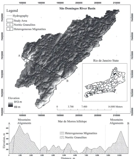
The study was carried out in an area of approximately 10,000 ha in the basin of the São Domingos River, a tributary of the Muriaé River in the northwestern region of the State of Rio de Janeiro, between the UTM coordinates 7,629,223N to 7,638,239N and 186,146E to 197,180E, Zone 24K, Datum Córrego Alegre (Figure 1). Two geomorphological systems can be found in the region: the hillslope area Mar de Morros and mountain chains and layered structures (NE-SW); the predominant lithology structure in the region comprise noritic granulites, heterogeneous migmatites and Quaternary alluvial deposits (DRM-RJ, 1980).
To understand the soil-landscape relationships, the area was surveyed according to procedures established for pedological surveys (Embrapa, 1995). For the characterization of the identified soil classes, 73 soil profiles and 11 extra samples were collected with augers and classified according to the Brazilian Soil Classification System (Embrapa, 2006). In view of the high number of soil classes and the high complexity of the training and validation processes, mainly for ANNs, as well as the limitations of the different programs used at each step, the area was subdivided (shown in table 1). The Quaternary deposit areas were considered to be the flattened patches in the areas of noritic granulites and heterogeneous migmatites.
This approach, which uses two different supervised classification algorithms (ANNs and the maximum likelihood algorithm), is based on the soil-landscape concept developed by Jenny (1941), according to which the soil is the result of interactions between formation factors over time.
Firstly, a digital elevation model (DEM) with a spatial resolution of 30 m was generated using the
Topo to Raster option of the ArcGIS 10 program
(ESRI, 2010). For this purpose, contour lines (20 m intervals), hydrography and elevation points contained in the topographic maps of IBGE SF-23-X-D-III-4 (Miracema) and SF-24-G-I-3 (São João do Paraíso) were used, both at a scale of 1:50,000. Then, after removing the spurious pits, this DEM was used to calculate the terrain attributes: elevation, slope, aspect, plan curvature and compound topographic index (CTI), according to Gallant & Wilson (2000), which together with the clay minerals, iron oxide (Sabins Junior, 1997) and Normalized Difference Vegetation Indices (NDVI) (Wiegand et al., 1991), derived from Landsat 7 ETM+ sensor imagery, represent the main factors of soil formation (discriminating variables) for the study area.
The compound topographic index (CTI) was obtained by equation 1:
(1)
where Asis the contributing area ((flow accumulation + 1) x cell size of the grid in m2) and βis the slope
expressed in radians.
The indices derived from the Landsat 7 ETM+ sensor images were used to reduce the work involved with data analysis by maximizing spectral information for a reduced number of sensor bands. Some studies demonstrated the relationship between the NDVI and soil moisture (Narasimha Rao et al., 1993) and the soil physical properties (Yang et al., 1997). This index was calculated as follows:
(2)
Similarly, clay minerals and iron oxide indices are frequently included in geological studies, underlying the distinction of soils with different physical and mineralogical characteristics (Sabins Junior, 1997). The clay mineral index was obtained by the ratio of band 5 (1.55-1.75 µm) by band 7 (2.08-2.35 µm) and the iron oxide index by the division of band 3 (0.63-0.69 µm) by band 1 (0.45-0.52 µm), both obtained from images of ETM+ sensor (LANDSAT 7) taken in
training process and avoid ANN saturation, as very large values can hamper the problem solution (saturation of the transfer functions could hinder the convergence of the network). Furthermore, efforts were made to prevent large variations in unimportant variables from inhibiting small variations in other more important variables.
The Java Neural Network Simulator was used for the classification by ANNs, based on the Stuttgart Neural Network Simulator 4.2 Kernel (Zell et al., 1996), and an applicable algorithm (funcpow) developed by Vieira (2000) for the classification by a Maximum Likelihood Classifier (MLC).
Two sets of independent stratified samples were collected from the areas containing profiles
considered to be representative of each soil class, one for the training process and the other for validation of the two classifiers. In this way, efforts were made to represent the characteristics of each one in relation to the discrimination variables used (elevation, slope, aspect, plan curvature, CTI index, clay mineral index, iron oxide index, and NDVI index). It should be highlighted that the soil classes differed in relation to one or more of the discriminating variables. The training samples were used so that the classifiers could establish relationships between the discriminating variables (input data) and the soil classes (output data) through a learning process. The validation samples were then used to test this relationship by statistical means.
The training samples for both classifiers consisted of 300 samples or pixels per class, i.e., 3,600 samples for Area 1 and 3,000 samples for Area 2. The number of validation samples was limited to 50 % of the number of training samples (150 samples or pixels per class), with 1,800 samples for Area 1 and 1,500 samples for Area 2, according to Zhu (2000).
In the training step, 10 ANN architectures were tested, which differed only in terms of the number of neurons in the internal layer (3, 5, 6, 7, 8, 9, 10, 15, 20, and 25 neurons). All of these had the same number of neurons in the input layer (number of discriminating variables) and in the output layer (12 soil classes for Area 1 and 10 for Area 2). The learning algorithm used was the backpropagation method, with random allocation of interneuron weights between -0.5 and -0.5 and a learning rate of 0.2, involving 10,000 learning cycles.
The results were evaluated through statistical means using the Kappa coefficient and overall classification accuracy, derived from a confusion matrix (Congalton & Green, 1999) from the validation samples. In this way, the ANN architecture obtaining the best result for the Kappa coefficient was selected for the prediction of the soil classes.
A statistical test to verify the significance of the differences between two or more classifiers (represented
by their respective confusion matrices) using Kappa coefficient analysis is proposed as an alternative approach for the comparison of independent confusion matrices. In this way, a significance matrix was generated using the results of the statistical tests for the chosen ANN and the classification with MLC, using the Kappa values and Kappa variance between the classifications, by means of the Z statistical test. The formula to test the significance between two independent Kappa coefficients (Z test) is given in the following equation:
(3)
Where Ka1 and Ka2 are the two Kappa coefficients
that are being compared (Congalton & Mead, 1986) and var is the variance of the Kappa coefficient (Ka). Thus, the Z test firstly verifies if the classification differs from a causal classification. In other words, if Z calculated < Zα/2 tabulated, the classification is
significantly better than a random classification, where α/2 is the confidence level of the Z test and the number of degrees of freedom is assumed to be infinite. In a second analysis, the test verifies if there is a significant difference between the Kappa values resulting from the evaluation by the different classifiers. Values < than 1.96 (95 % confidence level)
Symbol Soil class No. profiles and/or extra samples
Area 1 - Noritic granulites 39
AR1 Rock Outcrop
-CXbe typical eutrophic Tb Haplic Cambisol 5
GXbe solodic or typical eutrophic Tb Haplic Gleysol 2
LVAd typical dystrophic Red-Yellow Latosol 2
PAe1 typical eutrophic Yellow Argisol 2
PVe1 saprolitic eutrophic Red or Red-Yellow Argisol 2
PVe2 typical eutrophic Red Argisol 6
PVe3 nitosolic eutrophic Red Argisol 4
PVAe1 typical eutrophic Red-Yellow Argisol, highly undulating topography 4 PVAe2 typical eutrophic Red-Yellow Argisol, undulating topography 4
PVAd latosolic dystrophic Red-Yellow Argisol 6
RLe1 typical eutrophic Litholic Neosol 2
Area 2 - Heterogeneous migmatites 45
AR2 Rock Outcrop
-CXve typical eutrophic Ta Haplic Cambisol 10
GXve solodic or typical eutrophic Ta Haplic Gleysol 9
LVd typical dystrophic Red Latosol 2
PAe2 abruptic eutrophic Yellow Argisol 4
PVe4 saprolitic abruptic eutrophic Red Argisol 3
PVe5 abruptic eutrophic Red Argisol, highly undulating topography 7
PVe6 latosolic abruptic eutrophic Red Argisol 4
PVe7 abruptic eutrophic Red Argisol, undulating topography 4
RLe2 typical eutrophic Litholic Neosol 2
indicate no significant difference between the estimated Kappa values, while values > 1.96 demonstrate a significant difference.
The only existing soil survey in the area has a scale of 1:250,000 (Embrapa, 2003), a scale incompatible with the level of detail required for comparison with the digital maps produced by the two classifiers (between 1:100,000 and 1:50,000, medium scale). Therefore, 126 points of reference were used to determine the percentage of locations classified correctly on the maps, according to the procedure used by Zhu (2000). These reference points were collected by projects developed by Embrapa Solos in the area (the CNPq/CTHidro project, the Radema project and the Aquiferos project), including soil profiles, extra samples and observation points that were not used for the training and validation processes (independent points). The highest concentration of points in the middle of the area refers to a semi-detailed study carried out in the Barro Branco watershed for the Aquiferos project.
RESULTS AND DISCUSSION
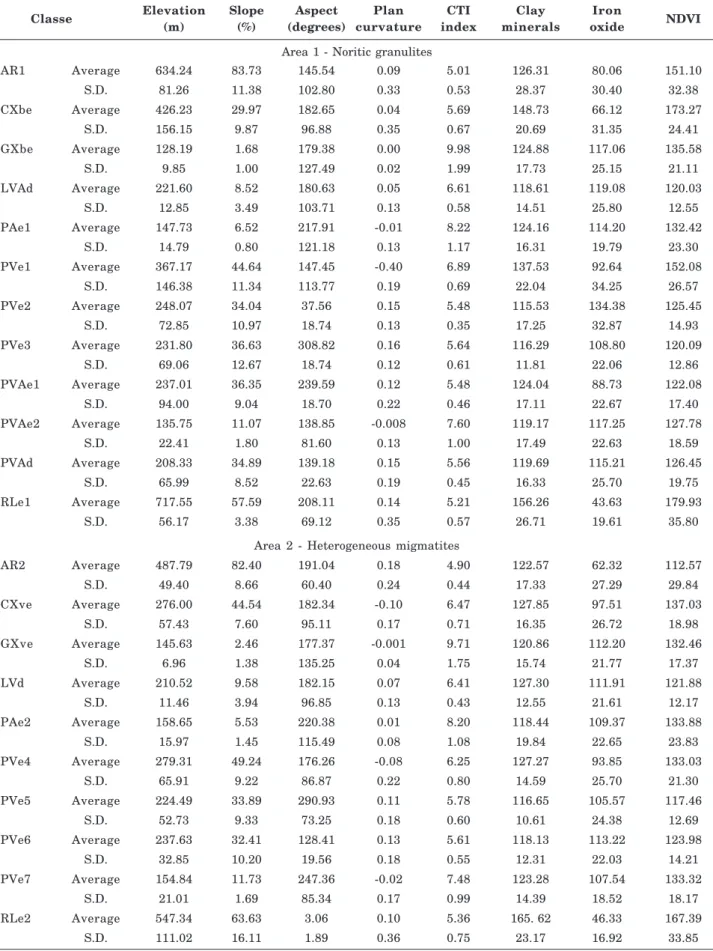
The contribution of the different variables in the discrimination of soil class in Areas 1 and 2 are shown in table 2.
In general, the differentiation of the soil classes detected by terrain attributes was much clearer than by the Landsat 7 indices. Studies carried out by Dobos et al. (2000, 2001) using terrain attributes and data from the Advanced Very High Resolution Radiometer (AVHRR) on the NOAA satellite for soil mapping showed that terrain attributes alone were not sufficient for the discrimination of the soils in the areas studied, while integrating this data with the AVHRR data increased classification performance.
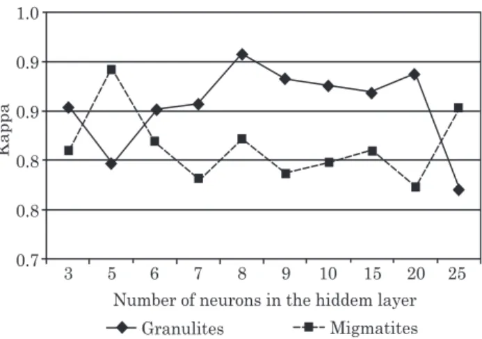
The best architecture for final data classification was selected based on the results of the Kappa coefficient and the overall accuracy, obtained using the validation samples (Figure 2).
In this evaluation, the highest values for the overall accuracy and the Kappa coefficient for Area 1, obtained using the validation samples, were achieved using network architecture with only one input layer containing 8 neurons (Kappa value of 0.908). The Kappa coefficient for Area 2 performed best when using a network architecture with an input layer containing five neurons (Kappa value of 0.893). An analysis of the Kappa significance matrix (Table 3) showed significant differences between these networks and the others. These two architectures were therefore selected for the final data classification.
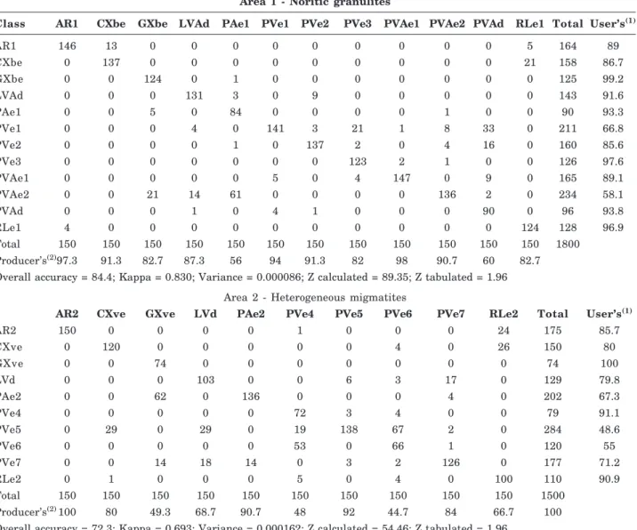
On the other hand, using MLC in the classification led to an overall accuracy of 84.4 % and a Kappa coefficient of 0.830 for Area 1, and an overall accuracy
of 72.3 % and a Kappa coefficient of 0.693 for Area 2. A comparison of the performances of the two classification types, based on an analysis of the Kappa significance matrix, indicated significant differences between these classifications for both areas (Table 4). The results obtained in this evaluation are similar to those in other studies, in which the approach via ANNs generally led to better results than by the MLC, mainly in the classification of soil use and cover using remote sensing data (Heermann & Khazenie, 1992; Bischof et al., 1992; Paola & Schowengerdt, 1995; McBratney et al., 2000).
Despite the significant differences between the two classifiers, with a better performance of the ANN classification (Kappa values of 0.908 and 0.893 for Areas 1 and 2 respectively), it should be emphasized that this approach requires more time and more computational resources for the training process than the classic approach using the MLC. However, for Yool (1998), ANNs have an advantage over conventional supervised classification methods such as MLC, as these are inadequate and impractical for the mapping of large areas.
According to Kanellopoulos & Wilkinson (1997), one aspect that has been neglected in the comparisons between statistical classifiers and artificial neural networks is the existence of significant differences in the performance of these classifiers when classes are considered individually. The confusion matrices obtained for the tested classifications based on the validation set are presented in tables 5 and 6.
In the area characterized by noritic granulites (Area 1), the worst performance for ANN classification occurred for class PAe1 (62.0 %), with greatest confusion with classes PVAe2, GXbe and LVAd. In the case of PVAe2 and GXbe, the confusion can be explained by the extremely similar characteristics of the discriminating variables between these classes, mainly for slope, CTI index and the indices derived from Landsat 7 (Table 2). For class LVAd, the differentiation was clearest with regard to elevation, slope and CTI index (Table 2); therefore, the confusion observed must be attributed to an error in the classifier. Accuracies exceeded 85 % for all other soil classes (Table 5).
In the area characterized by Heterogeneous Migmatites (Area 2), the worst performance occurred for class PVe5 (70.7 %), with greatest confusion with class PVe6 (Table 5). These classes have very similar environmental characteristics and can be differentiated only by their aspect (Table 2). Accuracies exceeded 95 % for all other soil classes (Table 5).
Classe Elevation Slope Aspect Plan CTI Clay Iron NDVI (m) (%) (degrees) curvature index minerals oxide
Area 1 - Noritic granulites
AR1 Average 634.24 83.73 145.54 0.09 5.01 126.31 80.06 151.10
S.D. 81.26 11.38 102.80 0.33 0.53 28.37 30.40 32.38
CXbe Average 426.23 29.97 182.65 0.04 5.69 148.73 66.12 173.27
S.D. 156.15 9.87 96.88 0.35 0.67 20.69 31.35 24.41
GXbe Average 128.19 1.68 179.38 0.00 9.98 124.88 117.06 135.58
S.D. 9.85 1.00 127.49 0.02 1.99 17.73 25.15 21.11
LVAd Average 221.60 8.52 180.63 0.05 6.61 118.61 119.08 120.03
S.D. 12.85 3.49 103.71 0.13 0.58 14.51 25.80 12.55
PAe1 Average 147.73 6.52 217.91 -0.01 8.22 124.16 114.20 132.42
S.D. 14.79 0.80 121.18 0.13 1.17 16.31 19.79 23.30
PVe1 Average 367.17 44.64 147.45 -0.40 6.89 137.53 92.64 152.08
S.D. 146.38 11.34 113.77 0.19 0.69 22.04 34.25 26.57
PVe2 Average 248.07 34.04 37.56 0.15 5.48 115.53 134.38 125.45
S.D. 72.85 10.97 18.74 0.13 0.35 17.25 32.87 14.93
PVe3 Average 231.80 36.63 308.82 0.16 5.64 116.29 108.80 120.09
S.D. 69.06 12.67 18.74 0.12 0.61 11.81 22.06 12.86
PVAe1 Average 237.01 36.35 239.59 0.12 5.48 124.04 88.73 122.08
S.D. 94.00 9.04 18.70 0.22 0.46 17.11 22.67 17.40
PVAe2 Average 135.75 11.07 138.85 -0.008 7.60 119.17 117.25 127.78
S.D. 22.41 1.80 81.60 0.13 1.00 17.49 22.63 18.59
PVAd Average 208.33 34.89 139.18 0.15 5.56 119.69 115.21 126.45
S.D. 65.99 8.52 22.63 0.19 0.45 16.33 25.70 19.75
RLe1 Average 717.55 57.59 208.11 0.14 5.21 156.26 43.63 179.93
S.D. 56.17 3.38 69.12 0.35 0.57 26.71 19.61 35.80
Area 2 - Heterogeneous migmatites
AR2 Average 487.79 82.40 191.04 0.18 4.90 122.57 62.32 112.57
S.D. 49.40 8.66 60.40 0.24 0.44 17.33 27.29 29.84
CXve Average 276.00 44.54 182.34 -0.10 6.47 127.85 97.51 137.03
S.D. 57.43 7.60 95.11 0.17 0.71 16.35 26.72 18.98
GXve Average 145.63 2.46 177.37 -0.001 9.71 120.86 112.20 132.46
S.D. 6.96 1.38 135.25 0.04 1.75 15.74 21.77 17.37
LVd Average 210.52 9.58 182.15 0.07 6.41 127.30 111.91 121.88
S.D. 11.46 3.94 96.85 0.13 0.43 12.55 21.61 12.17
PAe2 Average 158.65 5.53 220.38 0.01 8.20 118.44 109.37 133.88
S.D. 15.97 1.45 115.49 0.08 1.08 19.84 22.65 23.83
PVe4 Average 279.31 49.24 176.26 -0.08 6.25 127.27 93.85 133.03
S.D. 65.91 9.22 86.87 0.22 0.80 14.59 25.70 21.30
PVe5 Average 224.49 33.89 290.93 0.11 5.78 116.65 105.57 117.46
S.D. 52.73 9.33 73.25 0.18 0.60 10.61 24.38 12.69
PVe6 Average 237.63 32.41 128.41 0.13 5.61 118.13 113.22 123.98
S.D. 32.85 10.20 19.56 0.18 0.55 12.31 22.03 14.21
PVe7 Average 154.84 11.73 247.36 -0.02 7.48 123.28 107.54 133.32
S.D. 21.01 1.69 85.34 0.17 0.99 14.39 18.52 18.17
RLe2 Average 547.34 63.63 3.06 0.10 5.36 165. 62 46.33 167.39
S.D. 111.02 16.11 1.89 0.36 0.75 23.17 16.92 33.85
S.D.: standard deviation.
of the discriminating variables of these classes are very different (Table 2), it can be concluded that MLC was less efficient than ANNs in the discrimination of these classes. The confusion of class PAe1 was greatest with class PVAe2 (Table 6), in part related to the similarity of the discriminating variables between these classes (Table 2). Therefore, the result of ANNs for class PAe1 (62 %) suggests that MLC is less efficient.
In the area characterized by Heterogeneous Migmatites (Area 2), the worst performances were obtained for classes PVe6, PVe4 and GXve, with accuracies of 44.7, 48.0 and 49.3 % respectively. Accuracies of 83.3, 92.7 and 97.3 % were obtained using ANNs for the same classes, which shows that the MLC was less efficient than ANNs in the discrimination of these classes. For PVe6, the
Figure 2. Kappa coefficient obtained from the neural networks tested.
Area 1 - Noritic granulites
Network R3(1) R5 R6 R7 R8 R9 R10 R15 R20 R25
Overall accuracy 86.6 813 86.4 86.9 91.6 89.2 88.6 88.0 89.7 78.9
Kappa 0.85 0.80 0.85 0.86 0.91 0.88 0.88 0.87 0.88 0.77
Variance(2) 0.077 0.100 0.078 0.075 0.051 0.063 0.067 0.070 0.061 0.110
R3 97.21
R5 4.28* 79.60
R6 0.08 4.20* 96.47
R7 0.41 4.69* 0.49 99.07
R8 4.86* 9.11* 4.93* 4.45* 127.15
R9 2.45* 6.74* 2.53* 2.04* 2.44* 111.12
R10 1.92 6.19* 1.99* 1.51 2.95* 0.53 107.02
R15 1.32 5.60* 1.40 0.91 3.55* 1.13 0.60 103.87
R20 2.30* 6.62* 2.38* 1.89 2.65* 0.18 0.35 0.96 112.67
R25 6.07* 1.79 5.98* 6.47* 10.88* 8.52* 7.97* 7.38* 8.41* 73.42
Area 2 - Heterogeneous migmatites
Network R3 R5 R6 R7 R8 R9 R10 R15 R20 R25
Overall accuracy 82.8 90.4 83.7 80.4 83.9 80.8 81.8 82.9 79.6 86.8
Kappa 0.809 0.893 0.819 0.782 0.822 0.787 0.798 0.811 0.774 0.853
Variance(2) 0.117 0.071 0.112 0.128 0.11 0.126 0.121 0.116 0.132 0.094
R3 74.79
R5 6.13* 105.98
R6 0.66 5.47* 77.39
R7 1.73 7.87* 2.39* 69.12
R8 0.86 5.28* 0.20 2.59* 78.38
R9 1.41 7.55* 2.07* 0.31 2.28* 70.11
R10 0.71 6.86* 1.38 1.01 1.58 0.70 72.55
R15 0.13 6.00* 0.53 1.86 0.73 1.54 0.84 75.30
R20 2.22* 8.35* 2.88* 0.50 3.09* 0.81 1.51 2.35* 67.37
R25 3.03* 3.11* 2.37* 4.77* 2.17* 4.45* 3.75* 2.90* 5.26* 87.98
Table 3. Significance matrix for the different architectures tested
confusion with class PVe5 was greatest, as well as for GXve with PAe2 and PVe4 with PVe6 (Table 6). The MLC performed well in discriminating the other classes, despite some confusion, with accuracy values exceeding 78.7 %.
Finally, a comparison between ANN and MLC shows a differentiated classification in Area 1, with ANNs performing better for the classes AR1, GXbe, PAe1, PVe1, PVe2, PVe3, PVAd, PVAe2, and RLe1, while MLC was only better in the classification of CXbe and PVAe1. The LVAd was classified equally by the two classifiers (Tables 5 and 6). In Area 2, the ANN approach was better in the classification of all classes except PVe5.
According to Landis & Koch (1977), the Kappa coefficient value obtained through the neural network
Area 1 - Noritic granulites
Class AR1 CXbe GXbe LVAd PAe1 PVe1 PVe2 PVe3 PVAe1 PVAe2 PVAd RLe1 Total User’s(1)
AR1 147 0 0 0 0 0 0 0 0 0 0 5 152 96.7
CXbe 0 135 0 0 0 1 1 0 0 0 0 2 139 97.1
GXbe 0 0 143 4 10 0 0 0 0 0 0 0 157 91.1
LVAd 0 0 0 131 8 0 2 0 0 3 4 0 148 88.5
PAe1 3 0 6 5 93 0 0 0 0 1 0 0 108 86.1
PVe1 0 0 0 2 0 145 1 1 0 0 0 1 150 96.7
PVe2 0 0 0 0 0 0 144 6 0 0 3 0 153 94.1
PVe3 0 0 0 0 0 2 0 140 3 1 0 0 146 95.9
PVAe1 0 1 0 0 0 1 0 3 146 0 4 0 155 94.2
PVAe2 0 0 1 6 39 0 2 0 0 143 0 0 191 74.9
PVAd 0 0 0 0 0 0 0 0 1 2 139 0 142 97.9
RLe1 0 14 0 0 0 1 0 0 0 0 0 142 157 90.4
Total 150 150 150 150 150 150 150 150 150 150 150 150 1800
Producer's(2)98.0 90.0 95.3 87.3 62.0 96.7 96.0 93.3 97.3 95.3 92.7 94.7 Overall accuracy = 91.6; Kappa = 0.908; Variance = 0.000051; Z calculated = 127.14; Z tabulated = 1.96
Area 2 - Heterogeneous migmatites
AR2 CXve GXve LVd PAe2 PVe4 PVe5 PVe6 PVe7 RLe2 Total User’s(1)
AR2 150 2 1 0 0 1 0 0 0 0 154 97.4
CXve 0 145 2 3 0 3 0 0 0 0 153 94.8
GXve 0 2 143 1 0 7 3 0 0 0 156 91.7
LVd 0 1 0 139 7 1 0 0 0 0 148 93.9
PAe2 0 0 3 1 106 3 0 7 0 0 120 88.3
PVe4 0 0 1 6 24 125 0 9 0 0 165 75.8
PVe5 0 0 0 0 3 0 128 2 0 1 134 95.5
PVe6 0 0 0 0 10 9 17 130 4 2 172 75.6
PVe7 0 0 0 0 0 0 0 0 146 3 149 98.0
RLe2 0 0 0 0 0 0 2 2 0 144 148 97.3
Total 150 150 150 150 150 150 150 150 150 150 1500
Producer's(2)100 95.3 97.3 86.7 96 92.7 70.7 83.3 85.3 96.7
Overall accuracy = 90.4; Kappa = 0.893; Variance = 0.000071; Z calculated = 105.79; Z tabulated = 1.96
Table 5. Confusion matrix obtained via ANN classification
(1) User accuracy of a pixel classified in the image actually representing the same category in the field (Vieira, 2000); (2) Producer
accuracy of a pixel being correctly classified in its class. Classifier
Area 1 Area 2
Noritic Heterogeneous granulites migmatites
ANN MLC ANN MLC
Overall accuracy 91.6 84.4 90.4 72.3
Kappa 0.908 0.830 0.893 0.693
Variance 0.000051 0.000086 0.000071 0.000162
ANN 127.145 105.98
-MLC 6.66* 89.50 13.10* 54.45
Table 4. Significance matrix for the classifications carried out in the two areas studied
approach indicates a very good to excellent performance for this classifier (Kappa < 0.75) for both Area1 (0.908)
and Area 2 (0.893). On the other hand, the MLC presented a very good to excellent classification for Area 1 (0.830) and a moderate performance (0.4 <
Kappa < 0.75) for Area 2.
Considering that some classes occupy small and/ or very fragmented patches in the study area, some were grouped together to facilitate understanding of the ANN- and MLC-based maps. The criteria for this grouping was similarity in the characteristics of the area of occurrence, as mentioned in the key to Figure 3.
Although the results for the Kappa coefficient obtained from the validation samples were satisfactory for both classifiers, the resulting maps were different.
Area 1 - Noritic granulites
Class AR1 CXbe GXbe LVAd PAe1 PVe1 PVe2 PVe3 PVAe1 PVAe2 PVAd RLe1 Total User’s(1)
AR1 146 13 0 0 0 0 0 0 0 0 0 5 164 89
CXbe 0 137 0 0 0 0 0 0 0 0 0 21 158 86.7
GXbe 0 0 124 0 1 0 0 0 0 0 0 0 125 99.2
LVAd 0 0 0 131 3 0 9 0 0 0 0 0 143 91.6
PAe1 0 0 5 0 84 0 0 0 0 1 0 0 90 93.3
PVe1 0 0 0 4 0 141 3 21 1 8 33 0 211 66.8
PVe2 0 0 0 0 1 0 137 2 0 4 16 0 160 85.6
PVe3 0 0 0 0 0 0 0 123 2 1 0 0 126 97.6
PVAe1 0 0 0 0 0 5 0 4 147 0 9 0 165 89.1
PVAe2 0 0 21 14 61 0 0 0 0 136 2 0 234 58.1
PVAd 0 0 0 1 0 4 1 0 0 0 90 0 96 93.8
RLe1 4 0 0 0 0 0 0 0 0 0 0 124 128 96.9
Total 150 150 150 150 150 150 150 150 150 150 150 150 1800
Producer’s(2)97.3 91.3 82.7 87.3 56 94 91.3 82 98 90.7 60 82.7
Overall accuracy = 84.4; Kappa = 0.830; Variance = 0.000086; Z calculated = 89.35; Z tabulated = 1.96 Area 2 - Heterogeneous migmatites
AR2 CXve GXve LVd PAe2 PVe4 PVe5 PVe6 PVe7 RLe2 Total User’s(1)
AR2 150 0 0 0 0 1 0 0 0 24 175 85.7
CXve 0 120 0 0 0 0 0 4 0 26 150 80
GXve 0 0 74 0 0 0 0 0 0 0 74 100
LVd 0 0 0 103 0 0 6 3 17 0 129 79.8
PAe2 0 0 62 0 136 0 0 0 4 0 202 67.3
PVe4 0 0 0 0 0 72 3 4 0 0 79 91.1
PVe5 0 29 0 29 0 19 138 67 2 0 284 48.6
PVe6 0 0 0 0 0 53 0 66 1 0 120 55
PVe7 0 0 14 18 14 0 3 2 126 0 177 71.2
RLe2 0 1 0 0 0 5 0 4 0 100 110 90.9
Total 150 150 150 150 150 150 150 150 150 150 1500
Producer’s(2)100 80 49.3 68.7 90.7 48 92 44.7 84 66.7 100
Overall accuracy = 72.3; Kappa = 0.693; Variance = 0.000162; Z calculated = 54.46; Z tabulated = 1.96
Table 6. Confusion matrix obtained using validation samples for classification using the maximum likelihood algorithm
(1) User accuracy of a pixel classified in the image actually representing the same category in the field (Vieira, 2000); (2) Producer
accuracy of a pixel being correctly classified in its class.
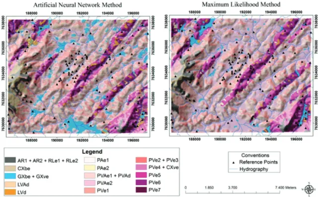
The agreement between the ANN- and MLC-based maps was only 47.28 %. According to Kanellopoulos & Wilkinson (1997), this low agreement demonstrates the differing nature of the mathematic models used in the classifications and the way they structure the space.
Figure 3 shows that both maps contain many spatial details, reported by Zhu (2000). Using terrain attributes and geological properties as discriminating environmental variables therefore showed the soil-landscape relationships in the area more clearly, resulting in spatially more detailed maps.
In the absence of a conventional soil map on an adequate scale ( < 50,000), reference points were used
Figure 3. Maps obtained by the two classifiers.
comparison, the classification using ANNs correctly inferred the soil classes at 93 locations (73.81 %) and MLC at 73 (57.94 %) (Table 6), which was comparable to results reported in other studies (Zhu, 2000; Zhu et al., 2001).
The matrix of Kappa significance (Table 7) indicated a significant difference between the classifiers. Better results were obtained using ANNs (Kappa coefficient of 0.709), which were significantly different from those obtained by MLC.
In the ANN classification, possible causes of the low agreement with the reference points include the rather complex geological nature of the area, which in some situations impeded the correct determination of soil-landscape relationships; the quality of the geological map used; the lack of information on the depth of lithic contact; and problems related to the environmental correlation model used. Most misclassified observations occurred at the boundaries between the units of the geological map. Problems related to the quality of geological maps used in environmental correlation studies were also reported by Thomas et al. (1999) and McKenzie & Ryan (1999).
McKenzie & Austin (1993) found that the presence of an impediment layer at low depths is a strong predictor of soil properties and the presence of geological structures such as dikes can control the soil distribution pattern. Dikes of basic material are common in the area studied, but are not shown on the geological map (DRM-RJ, 1980).
On the other hand, McKenzie & Ryan (1999) emphasized that there are circumstances in which soil variation occurs without any direct relation to easily observable environmental variables (lack of a reliable predictor) and in these cases, detailed sampling is inevitable and some form of interpolation is necessary to generate a spatial prediction.
In the case of MLC-based classifications, the low agreement with the reference points was mostly due to the inefficiency of the classifier.
The main lack of agreement between ANN- and MLC-based classifications can be verified in the flatter areas of the landscape (flat and gently undulating topography), classified by ANNs as belonging to the Haplic Gleysol class (GXbe and GXve for Areas 1 and 2 respectively) and by MLC as belonging to classes PVAe2 and PVe7 (for Areas 1 and 2 respectively), which occurs in undulating topography. In this case, the ANN-based classification was more accurate while MLC was less effective in adequately discriminating areas with very similar slope values.
Table 7. Confusion matrix between the maps obtained using ANN and MLC considering reference points
Classification ANNs MLC
Total number of points 126 126
Correctly classified points 93 73
Overall accuracy 73.81 57.94
Kappa 0.709 0.534
Variance 0.001826 0.002236
Neural network 16.59
Maximum likelihood 2.75* 11.29
* Significant difference of 95 %.
CONCLUSIONS
1. The Artificial Neutral Network classifier resulted in a higher accuracy for general classification when validation samples were used, producing significantly better statistical results than the Maximum Likelihood Classifier.
2. A comparison of reference points showed that the ANN-based was more accurate than the MLC-based map, which was significantly different. The main cause of data classification errors of the classifiers may be related to the geological heterogeneity of the area, the depth of lithic contact and problems associated with the environmental correlation model used, including the discriminating variables selected.
3. The use of terrain attributes and remote sensing data with spatial resolution compatible with the objectives of the study, together with a neural network approach, can help accelerate, extend and cheapen soil mapping in Brazil, due to the availability of lower-cost digital satellite images and the ease at which terrain attributes can be obtained.
LITERATURE CITED
ATKINSON, P.M. & TATNALL, A.R.L. Neural networks in remote sensing. Inter. J. Remote Sens., 18:699-709, 1997. BEHRENS, T.; FOSTER, H.; SCHOLTEN, T.; STEINRUCKEN, U.; SPIES, E.D. & GOLDSCHMITT, M. Digital soil mapping using artificial neural networks. J. Plant Nutr. Soil Sci., 168:21-33, 2005.
BENEDIKTSSON, J.A. & SVEINSSON, J.R. Feature extraction for multisource data classification with artificial neural networks. Inter. J. Remote Sens., 18:727-740, 1997.
BISCHOF, H.; SCHNEIDER, W. & PINZ, A.J. Multispectral classification of Landsat-images using neural networks. IEEE Trans. Geosci. Remote Sens.,30:482-490, 1992.
BORUVKA, L. & PENIZEK, V. A test of an artificial neural network allocation procedure using the Czech soil survey of agricultural land data. In: LAGACHERIE, P.; McBRATNEY, A. B. & VOLTZ, M., eds. Digital soil mapping: An introductory perspective. Amsterdam, Elsevier, 2007. p.415-424. (Developments in Soil Science, 31)
BRUS, D.J. & HEUVELINK, G.B.M. Optimization of sample patterns for universal kriging of environmental variables. Geoderma, 138:86-95, 2007.
CHAGAS, C.S.; FERNANDES FILHO, E.I.; VIEIRA, C.A.O.; SCHAEFER, C.E.G.R. & CARVALHO JÚNIOR, W. Atributos topográficos e dados do Landsat7 no mapeamento digital de solos com uso de redes neurais. Pesq. Agropec. Bras., 45:497-507, 2010.
CHAGAS, C.S.; CARVALHO JÚNIOR, W. & BHERING, S.B. Integração de dados do Quickbird e atributos do terreno no mapeamento digital de solos por redes neurais artificiais. R. Bras. Ci. Solo, 35:693-704, 2011.
CONGALTON, R.G. & GREEN, K. Assessing the accuracy of remotely sensed data: Principles and practices. New York, Lewis Publishers, 1999. 160p.
CONGALTON, R.G. & MEAD, R.A. A review of discrete multivariate analysis techniques used in assessing the accuracy of remotely sensed data from error matrices. IEEE Trans. Geosci. Remote Sens., 24:169-174, 1986. DEPARTAMENTO DE RECURSOS MINERAIS - DRM-RJ.
Projeto Carta Geológica do Estado do Rio de Janeiro na Escala 1:50.000. Folhas: Miracema e São João do Paraíso. 1980.
DOBOS, E.; MICHELI, E.; BAUMGARDNER, M.F.; BIEHL, L. & HELT, T. Use of combined digital elevation model and satellite data for regional soil mapping. Geoderma, 97:367-391, 2000.
DOBOS, E.; MONTANARELLA, L.; NÈGRE, T. & MICHELI, E. A regional scale soil mapping approach using integrated AVHRR and DEM data. Inter. J. Appl. Earth Obs. Geoinf., 3:30-42, 2001.
ELNAGGAR, A.A. & NOLLER, J.S. Application of remote sensing data and decision-tree analysis to mapping of salt-affected soils over large areas. Remote Sens., 2:151-165, 2010.
EMPRESA BRASILEIRA DE PESQUISA AGROPECUÁRIA -EMBRAPA. Centro Nacional de Pesquisa de Solos. Levantamento de reconhecimento de baixa intensidade dos solos do Estado do Rio de Janeiro. Rio de Janeiro, 2003. 242p. (Boletim de Pesquisa e Desenvolvimento, 32)
EMPRESA BRASILEIRA DE PESQUISA AGROPECUÁRIA -EMBRAPA. Centro Nacional de Pesquisa de Solos. Procedimentos normativos de levantamentos pedológicos. Brasília, 1995. 101p.
ENVIRONMENTAL SYSTEMS RESEARCH INSTITUTE -ESRI. ArcGIS Desktop. Redlands, 2010. v.10. GALLANT, J.C. & WILSON, J.P. Primary topographic
attributes. In: WILSON, J.P. & GALLANT, J.C., eds. Terrain analysis: Principles and applications. New York, John Wiley & Sons, 2000. p.51-85.
GIASSON, E.; SARMENTO, E.C.; WEBER, E.; FLORES, C.A. & HASENACK, H. Decision trees for digital soil mapping on subtropical basaltic steeplands. Sci. Agric., 68:167-174, 2011.
HEERMANN, P.D. & KHAZENIE, N. Classification of multispectral remote sensing data using a back-propagation neural network. IEEE Trans. Geosci. Remote Sens.,30:81-88, 1992.
HENGL, T.; TOOMANIAN, N.; REUTER, H.I. & MALAKOUTI, M.J. Methods to interpolate soil categorical variables from profile observations: Lessons from Iran. Geoderma, 140:417-427, 2007.
JENNY, H. Factors of soil formation; a system of quantitative pedology. New York, McGraw-Hill, 1941. 281p.
KANELLOPOULOS, I. & WILKINSON, G.G. Strategies and best practice for neural network image classification. Inter. J. Remote Sens., 18:711-725, 1997. LANDIS, J.R. & KOCH, G.G. The measurement of observer agreement for categorical data. Biometrics, 33:159-174, 1977.
McBRATNEY, A.B.; ODEH, I.O.A.; BISHOP, T.F.A.; DUNBAR, M.S. & SHATAR, T.M. An overview of pedometrics techniques for use in soil survey. Geoderma, 97:293-327, 2000.
McBRATNEY, A.B.; SANTOS, M.L.M. & MINASNY, B. On digital soil mapping. Geoderma, 117:3-52, 2003. McKENZIE, N.J. & AUSTIN, M.P. A quantitative Australian
approach to medium and small scale surveys based on soil stratigraphy and environmental correlation. Geoderma, 57:329-355, 1993.
McKENZIE, N.J. & RYAN, P.J. Spatial prediction of soil properties using environmental correlation. Geoderma, 89:67-94, 1999.
NARASIMHA RAO, P.V.; VENKATARATNAM, L.; KRISHNA RAO, P.V.; RAMANA, K.V. & SINGARAO, M.N. Relation between root zone soil moisture and normalized difference vegetation index of vegetated fields. Inter. J. Remote Sens., 14:441-449, 1993.
PAOLA, J.D. & SCHOWENGERDT, R.A. A detailed comparison of backpropagation neural network and maximum-likelihood classifiers for urban land use classification. IEEE Trans. Geosci. Remote Sens., 33:981-996, 1995. SABINS JUNIOR, F.F. Remote sensing: Principles and
interpretation. 3.ed. New York, W. H. Freeman and Company, 1997. 432p.
THOMAS, A.L.; KING, D.; DAMBRINE, E. & COUTURIER, A. Predicting soil classes with parameters derived from relief and geologic materials in a sandstone region of the Vosges mountains (Northeastern France). Geoderma, 90:291-305, 1999.
TSO, B. & MATHER, P.M. Classification methods for remotely sensed data. 2.ed. Boca Raton, CRC, 2009. 356p. WEINDORF, D.C. & ZHU, Y. Spatial variability of soil
properties at Capulin Volcano, New Mexico, USA: implications for sampling strategy. Pedosphere, 20:185-197, 2010.
WIEGAND, C.L.; RICHARDSON, A.J.; ESCOBAR, D.E. & GERBERMANN, A.H. Vegetation indices in crop assessments. Remote Sens. Environ., 35:105-119, 1991. YANG, W.; YANG, L. & MERCHANT, J.W. An assessment of
AVHRR/NDVI-ecoclimatological relations in Nebraska, USA. Inter. J. Remote Sens., 18:2161-2180, 1997. YOOL, S.R. Land cover classification in rugged areas using
simulated moderate-resolution remote sensor data and an artificial neural network. Inter. J. Remote Sens., 19:85-96, 1998.
ZELL, A.; MAMIER, G.; VOGT, M.; MACHE, N.; HUBNER, R.; DORING, S.; HERRMANN, K.; SOYEZ, T.; SCHMALZL, M.; SOMMER, T.; HATZIGEORGIOU, A.; POSSELT, D.; SCHREINER, T.; KETT, B.; CLEMENTE, G.; WIELAND, J. & GATTER, J. Stuttgart neural network simulator: User manual. Version 4.2. Stuttgart, University of Stuttgart, 1996. 338p.
TEN CATEN, A.; DALMOLIN, R.S.D.; PEDRON, F.A. & MENDONÇA-SANTOS, M.L. Regressões logísticas múltiplas: Fatores que influenciam sua aplicação na predição de classes de solos. R. Bras. Ci. Solo, 35:53-62, 2011.
ZHU, A.X. Mapping soil landscape as spatial continua: The neural network approach. Water Res. Res., 36:663-677, 2000. ZHU, A.X.; HUDSON, B.; BURT, J.; LUBICH, K. &