CINTAL - Centro de Investiga¸
c˜
ao Tecnol´
ogica do Algarve
Universidade do Algarve
CALCOM’10 Sea trial
Field calibration data report
P. Felisberto, S. Jesus, F. Zabel
Rep 04/10 - SiPLAB November/2010
University of Algarve tel: +351-289800131
Campus de Gambelas fax: +351-289864258
8005-139 Faro, [email protected]
Work requested by CINTAL
Universidade do Algarve, FCT - Campus de Gambelas 8005-139 Faro, Portugal
Tel/Fax: +351-289864258, [email protected],
www.cintal.ualg.pt
Laboratory performing SiPLAB - Signal Processing Laboratory
the work Universidade do Algarve, Campus de Gambelas,
8000 Faro, Portugal
tel: +351-289800949, [email protected], www.siplab.fct.ualg.pt
Projects WEAM (FCT PTDC/ENR/70452/2006)
Title Field Calibration Sea Trial WEAM’10: data report
Authors P. Felisberto, S. Jesus, F. Zabel
Date November, 2010
Reference 04/10 - SiPLAB
Number of pages 42 (forty two)
Abstract The CALCOM’10 sea trial took place in a region SSE of
Vilamoura from 22nd to 24th June to support WEAM & PHITOM projects. The first day was devoted to equipment testing and calibration. The second and third days were de-voted to field calibration and underwater communications. This report refers to field calibration data acquired 23rd June, Day 2, and 24th June, Day 3.
Clearance level UNCLASSIFIED
Distribution list SiPLAB(1+2DVDs), CINTAL (1+2DVDs),
WAVEC(1+2DVDs) Total number of copies 3 (three)
Contents
List of Figures V
Abstract 7
1 Introduction 9
2 The CALCOM’10 Sea Trial 11
2.1 The acquisition system . . . 12
2.2 Acoustic Signals . . . 13
2.2.1 Emitted signals . . . 13
2.2.2 Received signals . . . 14
2.3 Environmental data . . . 15
2.3.1 Day 2 - range independent bathymetry . . . 15
2.3.2 Day 3 - range dependent bathymetry . . . 16
3 Field calibration events 20 3.1 Day 2 . . . 21
3.2 Day 3 . . . 24
4 Acoustic channel modelling 27 5 Conclusions and Future Work 30 A Equipments specs 31 A.1 Acoustic Oceanographic Buoy - version 2 . . . 31
A.2 Acoustic source Lubell 1424 . . . 32
B SiPLAB VLA data files 34
IV CONTENTS
B.1 SipLAB VLA file format . . . 34 B.2 ReadVLA.m function . . . 34
C Experiment Log day 2 and day 3 36
C.1 Day 2 . . . 36 C.2 Day 3 . . . 38
List of Figures
2.1 CALCOM’10 work area off the south coast of Portugal. The working area for field calibration is bounded by the magenta square. . . 11 2.2 AOB22: after deployment, 24th June (a), schematics of AOB21 and AOB22
(b). . . 12 2.3 Acoustic source Lubell LL-1424: in a cage(a), installed in a tow fish (during
recovery) (b). . . 13 2.4 Spectrogram of the transmitted probe signal sequence used for field
cali-bration. . . 14 2.5 Spectrogram of the acoustic data received June 24, 12:57 pm, on hydrophone
8 of AOB22 at an approximate depth of 46 m and approximate source-receiver range of 5 km. . . 15 2.6 Day 2 bathymetry map of the work area with GPS estimated locations of
AOB21 (A1d) and AOB22 (A2d) deployments and their recovery (A1r,A2r), ship/source track (dotted line) and ship track during field calibration events (green lines). . . 16 2.7 Day 2 source depth and temperature (a), ship speed (b), AOB22
temper-ature data (c). . . 17 2.8 Day 3 bathymetry map of the work area with GPS estimated locations of
AOB21 (A1d) and AOB22 (A2d) deployments and their recovery (A1r,A2r), ship/source track (dotted line) and ship track during field calibration events (green lines). . . 18 2.9 Day 3 source depth and temperature (a), ship speed (b), AOB22
temper-ature data (c) . . . 19 3.1 Channel impulse response estimated from 500-1000 Hz lfm (a) and
1000-2000 Hz lfm (b), during the Day 2 event P2 at the hydrophone at 54 m depth of AOB21 . . . 21 3.2 Day 2 channel impulse response estimates along hydrophones from
500-1000 Hz lfm for AOB21 at source range 1.25 km (event P1) (a), 1.3 km (event P2)(b), 0.9 km (event P3) (c) and for AOB22 at source range 0.4 km (event P1) (d), 2.1 km (event P2) (e), 2.0 km (event P3)(f). . . 22 3.3 Day 2 channel impulse response estimates along source-receiver range at
hydrophone #3 (54 m) on AOB21 (event P2)(a), and at hydrophone #13 (55 m) on AOB22 (event P4) (b) . . . 23
VI LIST OF FIGURES
3.4 Bathymetry along the slope. The arrows show the location of the field calibration events and the receiver array (AOB22). . . 24 3.5 Day 3 channel impulse response estimates along hydrophones from
500-1000 Hz lfm at different events P1 (a), P2 (b), P3 (c), P4 (d), P6 (e) and (f). . . 25 3.6 Day 3 channel impulse response estimates along source-receiver range at
hydrophone #13 (54 m), at P6(a), and at P5 (b). . . 26 4.1 The environmental model of P6 used for simulations . . . 27 4.2 Modelled arrival patterns at hydrophone at 54m depth, with sediment
sound speed 1650m/s (a) and 1550m/s (c); and modelled arrival patterns for all hydrophones at 600m range, with sediment sound speed 1650m/s (b) and 1550m/s(d) . . . 28 4.3 Model outputs for the arrival pattern of hydrophone at 10m in Fig. 4.2(d):
amplitudes of modelled eigenrays with superimposed acquired arrival pat-tern (a), number of bottom and surface bounces (b) and eigenray paths (c). . . 29
Abstract
This report describes the acoustic field calibration data set acquired during the CAL-COM’10 sea trial, that took place off the south coast of Portugal, from 22 to 24 June, 2010. The CALCOM’10 sea trial was a joining effort of WEAM and PHITOM projects in-volving people from SiPLAB/CINTAL, WAVEC, ISR/IST Lisbon and Marsensing. This sea trial in addition to acoustic field calibration part described herein, encompassed acous-tic equipment testing and calibration and underwater communications testing, which are reported separately. Field calibration is a concept used to tune the parameters of an acous-tic propagation model for a region of interest. The basic idea is that one can accurate model the acoustic propagation in a given region with only a scarce apriori bathymetric and geoacoustic information of the area if relevant acoustic parameters obtained by acous-tic inference (i.e. acousacous-tic inversion) are integrated in the acousacous-tic model. For example, this concept can be applied to the classical problem of transmission loss predictions or, as in our case, the problem of predict the distribution of acoustic noise due to a wave energy plant. In such applications the accuracy of bathymetric and geoacoustic parameters esti-mated by acoustic means is not a concern, but only the accuracy of the predicted acoustic field. The objective of this approach is to reduce the need for extensive bathymetric and geoacoustic surveys, and reduce the influence of modelling errors, for example due to the bathymetric discretization used.
This report presents the experimental setup, the data acquired during the sea trial to prove the concept and discuss preliminary results of channel characterization and acoustic forward modelling. This work was supported by project WEAM (PTDC/ENR/70452/2006) funded by FCT, Portugal.
8
Chapter 1
Introduction
Nowadays there is an increasing demand for renewable energy sources. In this context the number of renewable energy installations in the ocean, off-shore wind mills and wave energy farms, will grow in the future. Such power plants, generally composed by several generators, will produce considerable acoustic noise that propagates through the ocean and will affect the oceanic environment to some extend. Started in November 2007 the project Wave Energy Acoustic Monitoring (WEAM) aims at developing, testing and vali-dating a monitoring system for determining underwater acoustic noise generated by wave generators and its impact in the sea fauna. The case study to be considered was initially the Pelamis installation off the Povoa de Varzim coast. Unfortunately, due to unforseen problems this installation was postponed and an alternative installation was considered: the 400 kW OWC pilot plant in Pico Island (Azores). Another objective of this project is to develop a methodology to predict the noise distribution on a candidate area for installation of a wave energy farm with several generators. The development of such a methodology will give rise to tools that will allow the developer/engineering team in an early phase of the project to predict the influence of such an installation in the environ-ment or decide about the optimal configuration in order to mitigate it. An initial model of noise distribution in a candidate area can be obtained by combining archival data, both hydrologic and seafloor, with outputs of oceanographic and acoustic modelling tools. How-ever, this initial acoustic noise model should be refined with actual measurements in the interest area, even in case that a large archival data set is available, otherwise most likely it will suffer from large errors due to the uncertainty of oceanographic and acoustic mod-elling. Although, several approaches can be considered to minimize the modelling errors, for instance based on frequent sound speed profile measurements, bottom surveys and cores and more powerful modelling tools, which are costly, herein an alternative method is considered. This alternative method, named (acoustic) field calibration consists in in-tegrating on the final acoustic noise predictions, results obtained from acoustic inversion of acoustic sensitive parameters, such as bathymetric and geoacoustic parameters. The idea is that, information of the environment obtained by acoustic inversion is sufficient and irreplaceable to attain an acoustic noise model of the area for the purposes consid-ered above. The field calibration method should be considconsid-ered a low cost method when compared with other methods that require detailed hydrological and seafloor surveys of the interest area.
One of the objectives of the sea trail CALCOM’10 was to obtain data to prove the field calibration concept. The chosen area is in the continental shelf off south Portugal, a perspective region to install wave energy farms in the future. The acoustic sampling of a squared area with a side of about 4km was obtained using two Acoustic Oceanographic Buoys (AOB) and a Lubell 1424 acoustic sound source. The AOBs are eight (AOB21) and sixteen (AOB22) hydrophone vertical arrays operated in free drifting mode. The sound source was towed from a boat emitting probe signals, sequences of chirps and
10 CHAPTER 1. INTRODUCTION
multitones in the 500-2000 Hz band. The movements of the boat were defined in order for the propagation paths to cover the different bathymetric and geoacoustic features of the area.
This report is organized as follows. Next chapter describes the field calibration part of the CALCOM’10 sea trial data set, including the experimental setup, and the acoustic and environmental data acquired. The chapter 3 presents estimations of the channel impulse response, while the chapter 4 an initial acoustic modelling effort. The conclusion and future work concludes this report. An additional DVD set contains the various data sets in mat-file format, which is described in appendix D.
Chapter 2
The CALCOM’10 Sea Trial
The CALCOM’10 sea trial took place off the south coast of Portugal, about 12nm south-east of Vilamoura, from 22th to 24th June 2010. The first day was used for test and calibration of equipment and the other two days for acquiring data to support field cal-ibration and underwater communication testing purposes. The working area for field calibration is represented by the magenta square in figure 2.1.
Figure 2.1: CALCOM’10 work area off the south coast of Portugal. The working area for field calibration is bounded by the magenta square.
The working area was chosen to be an approximately smooth and uniform area of constant depth around 100 m accompanying the coastline bathymetric contour surrounded by the continental relatively steep slope to the deeper ocean to the south. There are no specific information available for the bottom type of the working area, however taking into account geoacoustic classification found in maps for the region, one can expect a sandy/silty bottom with possible rocky patches.
12 CHAPTER 2. THE CALCOM’10 SEA TRIAL
2.1
The acquisition system
The acoustic system used to gather data for field calibration proposes was composed by two Acoustic Oceanographic Buoys (AOB) , vertical arrays with 8 (AOB21) and 16 (AOB22) hydrophones to acquired the data and the Lubell 1424 acoustic sound source and the Acoustic Emission and Reception Unit (AERU) .
Figure 2.2(a) shows the AOB22 after deployment, and figure 2.2(b) presents AOB21 and AOB22 schematics. The AOBs are ”intelligent” systems controlled by a PC104 pro-cessor board, with local data storage, wlan communications and possibility of autonomous unattended operation. AOBs are also equipped with GPS localization and timing system. Note that the 8 hydrophones in AOB21 are oddly distributed along the array at depths of 10, 15, 55, 60, 65, 75 and 80 m. The 16 hydrophones in AOB22 are equally spaced at 4 ˙m with the first hydrophone approximately at 6.3 m from sea surface. Moreover, AOB22 includes 16 low precision (0.5oC) temperature sensors collocated with hydrophones. The hydrophone has a flat frequency response from 1 Hz up to 28 kHz and the low noise differ-ential pre-amplifier has a constant gain of 40 dB in the whole frequency band of interest between 10 Hz up to 50 kHz.
(a) (b)
Figure 2.2: AOB22: after deployment, 24th June (a), schematics of AOB21 and AOB22 (b).
A summary of technical specs of the AOB systems can be found in appendix A.1, while a detailed description is given in [1, 2].
The source used to emit probe signals during the calibration part of CALCOM’10 sea trial was a Lubell LL-1424 sound source. A brief description and its frequency response this can be found in appendix A.2. The output power of the source is controlled by the supplied voltage. The AERU system [3] was used to generate the probe signals and control the source. During CALCOM’10 sea trial the Lubell LL-1424 was installed in a tow fish, since during part of the experiment the source was towed at a ship speed of 4 knots.
An autonomous recording device (Hobo) with a pressure and a temperature sensor was installed in the tow fish. This sensor allowed to monitor source depth, which is highly dependent on ship speed.
2.2. ACOUSTIC SIGNALS 13
(a) (b)
Figure 2.3: Acoustic source Lubell LL-1424: in a cage(a), installed in a tow fish (during recovery) (b).
2.2
Acoustic Signals
2.2.1
Emitted signals
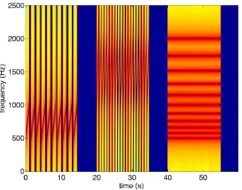
For field calibration purposes the probe signals were emitted in the 500-2000 Hz band. The signals consisted of a 1 minute sequences of linear frequency modulated (LFM) upsweeps and a mixture of tonal frequencies, known as multitones.
Figure 2.4 presents the spectrogram of a 1 minute long probe signal sequence. The output signal sampling frequency in the signal generator was set to 50kHz. Each sequence starts with a block of ten, one second long LFM in the band 500-1000 Hz, 250 ms apart. Follows a idle period of 5 s. The second signal block is composed by fifteen, half a second long LFM, in the band 1000-2000 Hz, 125 ms apart. A second idle period of 5 s follows the second signal block. The last signal block is a 15 s long mixture of 11 tones covering the 500-2000 Hz band at frequencies of 500.0, 574.3, 659.8, 759.9, 870.6, 1000.0, 1148.7, 1319.5, 1515.7, 1741.1, 2000.0 Hz. Also, after the signal block a idle period of 5 s is included in the signal sequence. Table 2.1 summarizes the 1 minute probe signal sequence. During field calibration events the sequences described above were continuously repeated in periods of
time signal duration start-end band Rep rate
(s) T (s) Freq. (Hz) (Hz)
0 LFM-Up 1 500-1000 500
1 blank 0.5 - - LFM 500-1000 & blank re10x
15 blank 5 - -
-20 LFM-Up 0.5 1000-2000 1000
20.5 blank 0.25 - - LFM 1000-2000 & blank 15x
35 blank 5 - -
-40 Multitones 15 500-2000 1500
-55 blank 5 - -
-60 end
14 CHAPTER 2. THE CALCOM’10 SEA TRIAL
Figure 2.4: Spectrogram of the transmitted probe signal sequence used for field calibra-tion.
about 15 minutes, with the ship drifting at station or moving at a speed bellow of 4 knots. A detailed description of the various events is presented in the next sections.
2.2.2
Received signals
The signals received at the hydrophones were acquired at a sampling frequency of 50 kHz. The acquired signals were stored in data files using SiPLAB proprietary format. In addition to acoustic data, the data file contains the non-acoustic data (temperature) and an ASCII header including cruise title, UTC GPS date and time of the first sample in file, GPS buoy positioning information (Lat, Lon), and characteristics of acoustic and non-acoustic data (number of channels, sampling frequency, sample size, total number of samples). The appendix B, describes the file format and the m-file ReadVLA.m used to read the data files to the Matlab c environment.
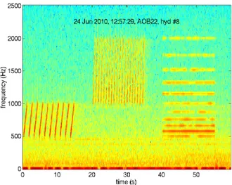
Since, the signals used for field calibration are bellow 2 kHz, the acoustic data were downsampled to 5 kHz. Figure 2.5 shows the spectrogram of a 1 minute sequence received on hydrophone 8 of AOB22 at an approximate depth of 46 m and approximate source-receiver range of 5 km.
2.3. ENVIRONMENTAL DATA 15
Figure 2.5: Spectrogram of the acoustic data received June 24, 12:57 pm, on hydrophone 8 of AOB22 at an approximate depth of 46 m and approximate source-receiver range of 5 km.
2.3
Environmental data
The two days of the CALCOM’10 sea trial described in this report were planned to perform transmissions at different bathymetric and source-receiver range configurations. In both days the AOBs were deployed 1 km apart, being the water depth in the site around 110 m. In June 23th, hereafter referred to as Day 2, the source, towed by the ship, moved at ranges within 2 km of the AOBs. The bathymetry was almost constant around 110 m depth. On day, June 24, hereafter referred to as Day 3, the ship towed the source from the receivers, toward the deepest part of the working area. The AOBs drifted 4.5 hours, attaining a maximum source-receiver distance of 5 km. The water depth increased with the distance from 110 m at the buoys location to 320 m at a range of 5 km. The bathymetry of the Algarve used in this report was available from the site http://w3.ualg.pt/∼ jluis/misc/Bat do Algarve 50m.zip. A GPS installed with the source system allowed to record the source (ship) movements and to determine the AOBs points of deployment and recovery. Although, GPS systems are installed in both AOBs, during Day 2, due to malfunction of the GPS board in case of AOB21 and malfunction of GPS antenna, in case of AOB22, it was not possible to record the positioning of the buoys. During Day 3, the GPS of AOB22 worked properly. The malfunction of the AOB21 GPS gave rise to a severe system problem that shut down the buoy few minutes after deployment.
Next, it is described for each day AOBs and source tracks, in particular the periods of 10-20 minutes, hereafter called events, when the signals used for field calibration were transmitted. Between field calibration events the resources were used for underwater communications events that will be reported separately. Also, the observations of the temperature array of AOB22, and the temperature and pressure sensor installed in the source tow fish are described in the following subsections.
2.3.1
Day 2 - range independent bathymetry
Figure 2.6 shows a bathymetry map of the work area and the location of the equipment. The star A1d represents the deployment position of AOB21 and the star A1r its recovery position. Similarly, the square A2d represents the deployment position of AOB22 and
16 CHAPTER 2. THE CALCOM’10 SEA TRIAL
Figure 2.6: Day 2 bathymetry map of the work area with GPS estimated locations of AOB21 (A1d) and AOB22 (A2d) deployments and their recovery (A1r,A2r), ship/source track (dotted line) and ship track during field calibration events (green lines).
the square A2d its recovery position. The buoys were deployed in a line of constant bathymetry. Since, the GPS systems of both AOBs did not work, those positions were given by the ship (source) GPS, and there is no positioning information for the AOBs between the deployment and recovery. The ship/source track is represented by the dotted line. The green lines over the ship track represent the source position during field cali-bration events. These events are labelled as P0, P1, P2, P3, P4. The location of the label represents the starting point of the event. Table 2.2 summarizes the time-location data for Day 2.
Figure 2.7(a) shows the temperature and the depth of source during Day 2. One can observe that the temperature at source depth was almost constant (17.6oC) during the
considered period. Regarding the source depth one can observe intervals where it was 7.5 m, and intervals where it was 9.0 m. In the former ones the ship is navigating, whereas in the later the ship is drifting (see ship speed in Fig 2.7(b)). Figure 2.7(c) shows the temperature acquired by the temperature sensor array of AOB22 along time, where one can observe periodic perturbation patterns similar to those related to internal waves as described in literature[].
2.3.2
Day 3 - range dependent bathymetry
The bathymetry of the area covered during Day 3 is shown in figure 2.8. This area is nearly 4 km east of Day 2 working area. The locations of AOB21 deployment and recovery are represented by a star, labelled A1d and A1r respectively. Unfortunately this buoy worked properly only a very short period after deployment. The squares represent the
2.3. ENVIRONMENTAL DATA 17
Events Lat. Lon. Lat. Lon. time time
start end start end start end
AOB21 36.8667 -8.1109 36.8643 -8.0908 10:29 16:11 AOB22 36.8714 -8.1005 36.8692 -8.0788 10:54 16:07 PO 36.8739 -8.0974 36.8749 -8.0956 11:40 11:54 P1 36.8750 -8.0948 36.8737 -8.0982 12:04 12:15 P2 36.8664 -8.1097 36.8644 -8.1162 12:44 13:06 P3 36.8607 -8.1077 36.8595 -8.1052 13:40 13:53 P4 36.8573 -8.1007 36.8627 -8.0922 14:18 14:40
Table 2.2: Day 2 time and location of equipments for field calibration.
(a) (c)
(b)
Figure 2.7: Day 2 source depth and temperature (a), ship speed (b), AOB22 temperature data (c).
18 CHAPTER 2. THE CALCOM’10 SEA TRIAL
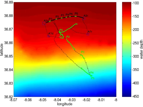
Figure 2.8: Day 3 bathymetry map of the work area with GPS estimated locations of AOB21 (A1d) and AOB22 (A2d) deployments and their recovery (A1r,A2r), ship/source track (dotted line) and ship track during field calibration events (green lines).
AOB22 point of deployment (A2d) and recovery (A2d). The AOB22 has drifted along the black curve. The water depth along this line is about 110 m. The dotted line represents the source/ship track during Day 3, which was along the bathymetric slope towards the south, with a water depth at the farthest location of about 320 m. During Day 3 the field calibration signals were transmitted during six periods 10-20 minutes long, called field calibration events. These events are labelled as P1, P2, P3, P4 P5, P6. The location of the label represents the starting point of the event. The green lines over the ship and AOB22 tracks represent the displacements of the ship and the buoy during the corresponding field calibration events. Table 2.3 summarizes the time-location data for Day 3.
The pressure and the temperature recorded at the source during Day 3 is shown in figure 2.9(a). Once can observe that the temperature is about 17.5oC with 0.5oC variations. The deepest source position is about 10.5 m and it occurs in intervals when the ship is drifting. When the ship is at cruise speed, ranging from 2 to 4 knots (Fig. 2.9(b)), the source depth decreases to depths ranging from 9 to 5 m. At 14 pm the source used to field calibration purposes was recovered and the sensor was installed in a high frequency source for communication purposes. The behavior is different, since this source was deployed and operated with yo-yo like displacements [4].
Figure 2.9(c) shows the temperature acquired by the temperature sensor array of AOB22 along time. The figure suggests that the AOB22 crossed a front in the middle of the period. Unfortunately, one can not validate this hypothesis with in-situ measurements of other instruments.
2.3. ENVIRONMENTAL DATA 19
Events Lat. Lon. Lat. Lon. time time
start end start stop start stop
AOB21 36.8649 -8.0462 36.8663 -8.0193 09:37 15:05 AOB22 36.8743 -8.0494 36.878 -8.0221 09:27 15:13 P1 36.8755 -8.0459 36.8761 -8.0447 10:11 10:27 P2 36.8772 -8.0414 36.8775 -8.0404 11:04 11:15 P3 36.8782 -8.0378 36.8783 -8.0367 11:45 11:56 P4 36.8787 -8.0345 36.8789 -8.0336 12:21 12:33 P5 36.8792 -8.0320 36.8794 -8.0311 12:53 13:03 P6 36.8796 -8.0284 36.8795 -8.0271 13:36 13:54
Table 2.3: Day 3 time and location of equipments during field calibration part of CAL-COM’10
(a) (c)
(d)
Figure 2.9: Day 3 source depth and temperature (a), ship speed (b), AOB22 temperature data (c)
Chapter 3
Field calibration events
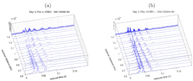
During field calibration events the one minute signal sequence covering the band 500-2000 Hz described in 2.2 were transmitted continuously in periods of 10-20 minutes in two days: 23th June, Day 2 and 24th June Day 3. The acoustic data acquired by the AOBs at a sampling frequency of 50 kHz were stored in SiPLAB proprietary file format (see appendix B). The received acoustic data were downsampled and separated in one minute mat files, where the different signals appear in the same sequence as at emission (500-1000 Hz lfm, 1000-2000 Hz lfm and 500-2000 Hz multitones (see section 2.2 for details). Incomplete received sequences that occurred at the beginning and at the end of field calibration events when the emitting system switched from/to communication signals were discarded. The impulse responses estimates of the acoustic channel, also known as arrival patterns, at distinct moments were obtained using 500-1000 Hz lfm and 1000-2000 Hz lfm, separately, by pulse compression. Since a reference hydrophone at source was not available, the signal loaded to the signal generator at the source system (see section 2.2) was used for pulse compression. The arrival patterns presented in next sections were calculated by averaging within a one minute interval. Thus, the arrival pattern corresponds to a 15 s averaging period for both type of lfm, where 10 single lfms in the 500-1000 Hz band and 15 single lfms in the 1000-2000 Hz were used. For each field calibration event the arrivals patterns as function of depth (hydrophone), and the arrival patterns at 55 m depth (3rd hydrophone of AOB21 and 13th hydrophone of AOB22) as function of source/receiver range. Since travel time is not available, the arrival patterns as function of range were aligned by the lag of maximum correlation between two adjacent arrival patterns.
A detailed analysis of the impulse response estimates of the different events is not in the scope of the present document. As general remarks one can say that, the a number of well known characteristics of underwater sound propagation channels are illustrated herein, such as the number of arrivals and their time spread as function of distance and water depth. Also, interference patterns like arrivals cancelling or the number of late arrivals in a packet as function of receiver depth or distance are present in a number of events. It is straightforward to see in Fig 3.1 that the shape of impulse response estimates obtained with both types of lfm (band 500-1000 Hz and 1000-2000 Hz) are similar, apart of higher resolution obtained with higher frequency lfm, which is due to its larger frequency band. Those arrival patterns were estimated during the Day 2 Event P2 at the 3rd hydrophone of AOB21 at 54 m.
.
Since the difference due to bandwidth is the major difference observed between arrival patterns estimated from 500-1000Hz lfm and 1000-2000 Hz lfm, in the next sections only the later will be presented.
3.1. DAY 2 21
(a) (b)
Figure 3.1: Channel impulse response estimated from 500-1000 Hz lfm (a) and 1000-2000 Hz lfm (b), during the Day 2 event P2 at the hydrophone at 54 m depth of AOB21
3.1
Day 2
Day 2 was devoted to short range transmissions, less than 2 km in an area with approx-imately 110 m water depth and small bathymetric gradients, thus almost range indepen-dent bathymetry (see section 2.3.1).
Both AOBs acquired acoustic data, but due to systems malfunction there is a lack of accurate GPS positioning and time information in the data files. The instants of the Day 2 events are only roughly estimated. Moreover, the position of the AOBs along their tracks is obtained by linear interpolation using the time and position of AOBs at place of deployment and recovery given by source/ship GPS. One can expect offsets of several minutes in time, and errors of hundred of meters in positioning. Thus, the information derived from time/positioning information, like source receiver range, source receiver bathymetry, source depth and temperature at source in an interval or mean temperature profile can be affected by time biases and positioning errors.
Also note that during Day 2 the external power source used in the ship was not able to supply sufficient instantaneous power at peaks required by the acoustic source transmission system. This problem that gave to abnormal signals transmitted in water, specially in bands used by ucomms.
Figure 3.2 presents the channel impulse responses obtained at Day 2 along the hy-drophones on both buoys at events P1, P2 and P3. One can note that the number of peaks in the different arrival patterns are well resolved. The number and time spread of arrivals increase with the distance and for similar distances their structure is similar, not depending on the event. Since the water depth is almost constant in the Day 2 work area, it should indicates that also the bottom characteristics are similar along the acoustic paths. It is also straightforward to see, specially in AOB21 arrival patterns, that due to arrivals interference the amplitude of the first peak of arrival patterns varies with depth: their amplitudes increase with depth. As expected the amplitude of the strongest peaks decreases with distance.
Figure 3.2 also shows the arrival fronts impinging the array and their direction. The later arrival fronts show steepest angles, since they are related to rays that suffer several surface and bottom reflections. The number of arrivals in each arrival packet and their separation in time depends on the depth of the hydrophone.
22 CHAPTER 3. FIELD CALIBRA TION EVENTS
(a) AOB21 @ 1.25 km (b) AOB21 @ 1.3 km (c) AOB21 @ 0.9 km
(d) AOB22 @ 0.4 km (e) AOB22 @ 2.1 km (f) AOB22 @ 2 km
Figure 3.2: Day 2 channel impulse response estimates along hydrophones from 500-1000 Hz lfm for AOB21 at source range 1.25 km (event P1) (a), 1.3 km (event P2)(b), 0.9 km (event P3) (c) and for AOB22 at source range 0.4 km (event P1) (d), 2.1 km (event P2) (e), 2.0 km (event P3)(f).
3.1. DAY 2 23
(a) (b)
Figure 3.3: Day 2 channel impulse response estimates along source-receiver range at hydrophone #3 (54 m) on AOB21 (event P2)(a), and at hydrophone #13 (55 m) on AOB22 (event P4) (b)
At shallow hydrophones, the surface reflected arrival fronts interferes with bottom re-flected ones and two packets of two arrivals merge into a single packet of four or three arrivals. It is straightforward to see that a similar interference occurs at deeper locations, which are not sampled by the array.
Figure 3.3 presents impulse response estimates along source-receiver range at hydrophones at an approximately depth 54 m for AOB211 (event P2), Fig. 3.3(a), and for AOB22 (event P4), Fig. 3.3(b). One can observe that arrival patterns are stable along source-receiver range, and the number of arrivals and their time spread increases with distances. One can also note that the interference in the first peak, previously observed along the hydrophones, also occurs along source-receiver range.
24 CHAPTER 3. FIELD CALIBRATION EVENTS
Figure 3.4: Bathymetry along the slope. The arrows show the location of the field calibration events and the receiver array (AOB22).
3.2
Day 3
Except for the last field calibration event were the source-receiver bathymetry was nearly flat, during the initial five events P1-P5 signals were transmitted along bathymetric up slope from the source to receiver locations, Fig 3.4. The longest source-receiver distance was 5 km.
At Day 3 the AOB21 computer system shut down few minutes after deployment, thus only data at event P1 is available. This data will not be presented herein, but the acoustic data gathered can be considered for future processing, since it seems of good quality. GPS time and position is not available in event P1 for AOB21 data.
Note that the dynamic range of the ADC of the hydrophones and the output power of the acoustic source were changed during the day (see appendix C for details).
Figure 3.5 presents arrival patterns observed at the different events, thus at different source-receiver ranges, along the batymetric slope. In general, the comments made for Day 2 observations apply here. One can notice that the arrival patterns are stable, the peaks are well resolved and as expected the number and time spread of arrivals increase with distance, whereas the amplitude of the peaks decreases. Also, the later arrival fronts show steepest angles, since they are related to rays that suffer several surface and bottom reflections. The number of arrivals in each arrival packet and their separation in time depends on the depth of the hydrophone. At shallow hydrophones, the surface reflected arrival fronts interferes with bottom reflected ones and two packets of two arrivals (single arrival in Fig.3.5(d)) merge into a single packet of four or three arrivals (two arrivals in Fig.3.5(d)). One can also observe a cancelling interference in the first peak along the hydrophones, being the first peak cancelled at shallowest hydrophones in Fig. 3.5(a)) and Fig. 3.5(f)). This interference is more complex in Fig. 3.5(d), where the amplitude of first peak in hydrophones in the middle of the array is smaller than in shallower hydrophones. At deeper hydrophones the single peak becomes two separated peaks.
3.2. D A Y 3 25
(a) AOB22 @ 1.1 km, P1 (b) AOB22 @ 1.8 km, P2 (c) AOB22 @ 3.25 km, P3
(d) AOB22 @ 5 km, P4 (e) AOB22 @ 1.6 km, P6 (f) AOB22 @ 0.6 km (P6)
Figure 3.5: Day 3 channel impulse response estimates along hydrophones from 500-1000 Hz lfm at different events P1 (a), P2 (b), P3 (c), P4 (d), P6 (e) and (f).
26 CHAPTER 3. FIELD CALIBRATION EVENTS
(a) (b)
Figure 3.6: Day 3 channel impulse response estimates along source-receiver range at hydrophone #13 (54 m), at P6(a), and at P5 (b).
Figure 3.6 shows arrival patterns along source-receiver distance observed on hydrophone at depth 54 m in two different events P6, Fig. 3.6(a), and P5, Fig. 3.6(b). In the former, the source-receiver paths are in shallow water. One can observe that the number of arrivals and their time spread increases with the distance, the cancelling interference in the first peak occurs with increasing distance. In the later, because the source-receiver paths are along the bathymetric up slope and the closest and farthest distance are only a fraction of the source-receiver ranges, the arrival patterns are very similar. The number of arrivals and their time spread in Fig. 3.6(b) is greater than in Fig. 3.6(a) because of longer source-receiver range in the former, but the amplitude of the peaks are smaller.
Chapter 4
Acoustic channel modelling
Next it is presented preliminary results of modelling acoustic channel impulse responses for a typical situation found in the previous chapter.
The environmental setup used for simulations, depicted in Fig. 4.1, is based on the conditions of event P6: source-receiver range between 0.6 and 1.6km, source depth 7m, water depth ranging from 109m at receiver location to 125m at a receiver range of 1.6km. The sound speed profile considered in simulations is the mean sound speed profile derived by the Mackenzie formula from the temperature data acquired by the temperature sensor array at the receiver, assuming a constant salinity of 36ppm for the layers covered by the array and the mean profile described in reference [5] for the deeper layers. The source range was derived from GPS information, the source depth from the pressure sensor at the source, the bathymetry from the available bathymetry map.
Figure 4.2 presents the modelled arrival patterns under the same conditions as those of Fig. 3.5(f) and Fig. 3.6(a). The arrival patterns were modelled using the Bellhop ray tracing model.There is no available detailed sea bottom data for the region, only a descriptive classification can be found [6]. The bottom is described as silty, thus it is assumed a sediment (compressional) sound speed of 1650m/s, a density of 1.7 and an attenuation of 1.0 dB/l. The modelled arrival patterns obtained are shown in Fig 4.2 (a) and (b), which compare favorably with Fig 3.6(a) and Fig 3.5(f), respectively. One can observe that the structure of observed and modelled arrival is similar, but the number and strength of late arrivals is greater in modelled arrival patterns than in the observed ones, which suggests that the bottom is softer than the bottom assumed in the model. Figure 4.2(c) and (d) show the modelled arrival patterns where the bottom sound speed was changed to 1550m/s, and density to 1.5. The attenuation was unchanged. It is straightforward to see that the match between the modelled structure of late arrivals and
Figure 4.1: The environmental model of P6 used for simulations 27
28 CHAPTER 4. ACOUSTIC CHANNEL MODELLING
(a) (b)
(c) (d)
Figure 4.2: Modelled arrival patterns at hydrophone at 54m depth, with sediment sound speed 1650m/s (a) and 1550m/s (c); and modelled arrival patterns for all hydrophones at 600m range, with sediment sound speed 1650m/s (b) and 1550m/s(d)
29
(a) (c)
(b)
Figure 4.3: Model outputs for the arrival pattern of hydrophone at 10m in Fig. 4.2(d): amplitudes of modelled eigenrays with superimposed acquired arrival pattern (a), number of bottom and surface bounces (b) and eigenray paths (c).
observed ones resulted improved with the new value of the sediment sound speed. Another interesting feature observed on the arrival patterns in Fig. 3.6(a) is the cancellation of the first arrival in hydrophones close to the surface. In modelled arrival patterns the first arrival do not cancel totaly, however the strength of the first arrival in hydrophones close to the surface is smaller than in deeper hydrophones.
The model outputs relative to the arrival pattern for the hydrophone at 10m in Fig 4.2(d) are shown in Fig. 4.3: amplitude-delay of the eigenrays (a), their number of bounces (b) and paths (c). On can see, that the first peak on the arrival pattern is due to direct eigenrays and surface reflected eigenrays. Although the amplitudes of that first packet of arrivals estimated by the model are the greatest, due to their relative phases and relative instant of arrival, they sum destructively. In fact, due to the sound speed profile and/or source/receiver depth and distance this packet of arrivals can be cancelled at all, what most likely happens in arrival patterns observed in Fig. 3.5(f). The arrival pattern in Fig. 3.5(f) relative to the hydrophone at depth 10 m is superimposed to eigenray amplitude-delay plot in Fig 4.3(a). Despite the amplitude of the first arrival, the structure of modelled and observed arrivals is in good agreement. The amplitude of the latest packet of arrivals (centered at 0.6s) predicted by the model is small due to several reflections (3) in the bottom, thus it is embodied in the noise in the observed arrival pattern (not shown).
Chapter 5
Conclusions and Future Work
This report describes the field calibration part of the CALCOM’10 experiment. presented acquired during the CALCOM’10 experiment. The preliminary data analysis of the field calibration data set shows good quality data, sampling the interest area in a convenient way in order to quantify its variability by acoustic inversion. A preliminary forward modelling showing good agreement with the acquired data is also presented. The next step in processing this data set is to systematically estimate relevant parameters to acoustically characterize the interest area. The ultimately objective is to develop a tool to be used at developing stage and to allow developers to optimize the number and location of wave energy generators and predict their influence in underwater noise in surrounding areas.
Appendix A
Equipments specs
A.1
Acoustic Oceanographic Buoy - version 2
Name AOB
Version 2
Model 001 (002)
Type Acoustic VLA
Aperture 80 m (66 m)
No. sections 1 (1)
No. channels 8 (16)
Hydrophone depths (m)
model 001 10,15,55,60,65,70,75,80
model 002 hyd 1 at 6 m, spacing 4m
Frequency band 0 - 25 kHz
Sampling frequency 60 kHz (GPS synchro)
AD conversion 16 bits Bit rate 7.68 (15.36) Mb/s Battery 48 Ah Autonomy 11 to 13 h Data storage 80 (120) GB Wirelesslan 802.11b Wirelesslan amp. 1 W
Wirelesslan antenna omni 7 dBi
Weight (air/water) 41.4 / 10 Kg
Height w/mast 300 cm
Width w/ float 40 cm
Ballast 10 Kg
32 APPENDIX A. EQUIPMENTS SPECS
A.2
Acoustic source Lubell 1424
Lubell.com Presents
Lubell LL-1424HP
Underwater Acoustic
Transducer
High-Power Broadband Piezoelectric Underwater transducer for Military and
Scientific Applications
SPECIFICATIONS
Frequency Range: 200Hz - 9kHz
(+/-4dB between 400Hz - 8kHz)
SPL: 197dB/uPa/m @ 600Hz (80V rms
applied at cable end)
Maximum Voltage: 80 Vrms Duty Cycle: 100%/10A, 50%/14A Impedance: 8 ohms nominal (including
AC1424HP xfmr box)
Depth Rating: 6' - 40'
Dimensions: 16.5" x 16.5" x 16.5" Ducer/Cage Wt: 61 lbs/air, 33 lbs/water Finish: 10-mil epoxy on MIL-C-5541
Class 1-A (transducer); 304SS cage
Connector: Seacon XSEE3BCR
Cable: Seacon XSEE3CCP molded to one end of 50 meter 14/3 SO cable (32 lbs)
Data: Guide, TVR, SPL, Z, tabular
Included: CLX4 amplifier, 2800 watts @
4 ohms (105 Vrms) 100-240VAC 50/60 Hz operation, AC1424HP bridging xfmr box.
Option: Swagelok SS-400-1-OR pressure fitting with SS-400-P plug ($100) allows connection to aftermarket bladders.
Price: $8499
Warranty: 2 year limited
Contact: Lubell Labs Inc.
Tel: (614) 235-6740, 9:00am-5:00pm EST
Printable PDF brochure
The LL-1424HP is a piezoelectric underwater acoustic transducer designed for general purpose military and scientific applications. The LL-1424HP may also be used as an underwater speaker when high power is required.
The LL-1424HP has a useful frequency range of 200Hz-9kHz (400Hz-8kHz +/-4dB), a maximum SPL of 197dB/uPa/m @ 600Hz w/80V rms applied, and a nominal impedance of 8 ohms. The LL1424HP is now provided with an AC1424HP bridging transformer box and CLX4 amplifier for worldwide use. The LL-1424HP is built to withstand ocean environments by virtue of its 10 mil epoxy finish, and EPDM shock mounting in stainless steel cage. The LL-1424HP is fitted with a Seacon bulkhead connector and includes a mating 50 meter Seacon cable. The LL-1424HP operates at depths up to 10 meters, and may be ordered with Swaglok fitting allowing bladder compensation at greater depth.
Appendix B
SiPLAB VLA data files
This section describes the SiPLAB VLA file format and the ReadVLA Matlab function which is used to retrieve acquired acoustic and non-acoustic data from the SiPLAB equip-ment data files (VLA).
B.1
SipLAB VLA file format
The SiPLAB data files are structured into two sections, the header and the payload. The header is composed of the first 4 lines of the file and is in ascii format as can be seen in table B.1.
UAN10 Engineering Sea Trial - (Pianosa) Mon, 20 Sep 2010,
12:45:37.000000 Lat 00.0000N Lon 0.0000W nonACOUSTIC Fs:00000
NoSens:00 SampSz:32 TotS:00000000 ACOUSTIC Fs:60000 NoSens:12
SampSz:24 TotS:21503160
Table B.1: SiPLAB data file Header Example
The first line in the header is a textual description including the name of the experiment and the location. The second line includes a date/timestamp which is as precise as the equipment which created it (refer to equipment specifications), GPS location is also included in this line in decimal degree format. The third line is in respect to the non acoustic sensors and includes information like sampling rate, number of sensors, the size in bits of each sample and the total number of samples.The forth line is in respect to the acoustic sensors and includes information like sampling rate, number of sensors, the size in bits of each sample and the total number of samples.
B.2
ReadVLA.m function
The ReadVLA function (refer to table B.2) is used through the following syntax: [data, Fs, NoSs, TITLE, TIMEPOS]=ReadVLA(filename, DataType)
B.2. READVLA.M FUNCTION 35
Table B.2: ReadVLA.m function [data, Fs, NoSs, TITLE,
TIMEPOS]=ReadVLA(filename,DataType) %
% Reads a Data File from the SiPLAB VLA files %
% [data, fs, NoSs, TITLE, TIMEPOS]=ReadVLA(file,flag) %
% Where:
% data: is a matrix [ NoChannels * Total No Samples ]
% fs: sampling frequency
% NoSs: Number of Channels
% TITLE: Description of the experiment
% TIMEPOS: Time/Position information of the data in the file %
% file: name of file to be read, empty variable will allow theselection
% of the file to read, recognized extensions:
% * ".acust" - Acoustic Data
% * ".tilt1"/".tilt2" -Array Inclination Data % * ".pr1"/".pr2" -Array Depth Data
% * ".temp" - Temperature Data
% * ".dummy" - Battery Voltage Data
% flag: if greater than 0, return values of data will be converted % to its usable System Units ( volts, degrees of inclination,meters, etc ) %
where filename is the name of the VLA file and DataType should be specified as ’acous-tic’ or ’nonacous’acous-tic’ in respect to the data which should be read. The function return the variables:
’data’ - actual data ’Fs’ - Sampling Rate
’NoSs’ - Number of Sensors ’TITLE’ - The ascii description
Appendix C
Experiment Log day 2 and day 3
C.1
Day 2
All times in this log are in GMT / UTC. During this experiment 3 signal sets were transmitted which are referred to as ’1’ for field calibration, ’2’ and ’3’ for ucomms. Two Buoys (AOB21 and AOB22) were deployed during this day. AOB21 was configured with an ADC input of +-2V which corresponds to a gain of 5x. AOB22 was also configured with a gain of 5x.
Additional Notes relating to operations:
• AOB22 - GPS was not functional during the experiment, only initial and final • location can be determined, use AOB21 movement for aproximate path. • AOB22 - files are not time sync because of missing GPS
• AOB22 the Time on Buoy 2 23,06,2010 03:13 corresponds + to 10:54 GMT -difference of 7h 41min
• AOB21 - GPS was later identified as having incorrect results with incorrect data reception
C.1. DAY 2 37
Table C.1: Day2 - Operations Log
10:29 AOB21 in water
10:54 AOB22 in water
11:40:xx TX Sound
12:02:xx placed pressure sensor on LF source 12:05:xx start of LF Tow 12:15:42 Stop Signal 1 12:16:00 Load Signal 2 12:29:09 Stop Signal 2 12:29:39 Load Signal 3 12:43:00 Stop Signal 3 12:44:xx Load Signal 1 12:44:30 Signal 1 started ? 13:00:xx ? station C1 - signal 1 13:07:00 Stop Signal 1, Load Signal 2 13:10:xx +- start signal 2
13:20:xx Stop Signal 2, Load Signal 3 13:22:xx +- start signal 3
13:33:xx stop station C1, start transit 13:34:xx Load signal 1
13:42:xx station C2, tx signal 1 13:53:xx stop signal 1, load signal 2 13:55:xx +- start signal 2
14:06:xx stop, reload signal 3 ?
14:20:xx END STATION C2, loaded signal 1
14:40:xx stop signal 1, load signal 2, LF-source still in Tow
14:52:xx recovered LF source stopped at position 36 51.7256’ N 8 5.2240’ W 14:54:xx placed hobo pressure sensor on HF source
14:55:xx Lubell HF test
15:00:00 start tx PASU HF source 15:19:00 jpg signals
15:30:40 start 5x repeat salman 15:46:20 start 5x repeat jpg
16:03:32 start AOB22 recovery (GPS NOT OK) 16:07:00 AOB22 out of the water
38 APPENDIX C. EXPERIMENT LOG DAY 2 AND DAY 3
C.2
Day 3
All times in this log are in GMT / UTC. During this experiment 3 signal sets were transmitted which are referred to as ’1’ for field calibration, ’2’ and ’3’ for ucomms. Two Buoys (AOB21 and AOB22) were deployed during this day. AOB21 was configured with an ADC input of +-2V which corresponds to a gain of 5x. AOB22 was also configured with a gain of 5x.
09:27:22 AOB22 in water 09:xx:xx AOB21 in water 10:14:xx Tx with 35V @6.7A 10:15:xx Tx Signal 1
10:17:40 Changed AOB21 to +-1V gain 10x
10:19:31 Start of tow of LF source in direction of AOB22 10:2x:xx changes TX to 42V @8.1A
10:28:xx stop signal 1, load signal 2 10:30:xx +- start tx signal 2, 22V @ 7.6A 10:43:xx Stop tx signal 2, load signal 3 10:46:xx start tx signal 3, 12V @7A 11:03:40 stop tx signal 3
11:04:59 start tx signal 1
11:17:00 stop tx signal 1, load signal 2 11:17:xx 150 m water depth
11:18:50 +- start tx signal 2 11:19:00 Station RD1
11:31:30 stop tx signal 2, load signal 3 11:33:55 start tx signal 3
11:45:00 stop signal 3, load signal 1 11:46:00 start tx signal 1
11:53:30 boat started for next mile 11:57:00 stop signal 1, load signal 2 11:59:20 start tx signal 2
12:09:30 stop tx signal 2, loaded signal 3 12:16:04 boat stopped at station RD2 12:16:xx 289 m water depths
12:21:00 stop tx signal 3, load signal 1 12:22:25 start tx signal 1
Table C.2: Day3 - Operations Log Additional Notes relating to operations:
• AOB21 stopped working @10:24 for an unknown reason, also GPS on AOB21 was not functional.
C.2. DAY 3 39
12:33:30 stop tx signal 1, load signal 2 12:36:00 start signal 2
12:41:00 Generator OFF, added fuel
12:50:00 Restart of systems, and start of ship movement 12:53:00 loaded signal 1
12:53:59 start tx signal 1
13:03:40 stop signal 1, load signal 2 13:06:xx +- start of signal 2
13:16:30 stop signal 2, load signal 3 13:16:xx start of tow @ 4knots 13:18:55 start signal 3
13:18:xx changed tow to 2knots 13:35:41 stop signal 3, load signal 1 13:36:41 start signal 1
13:36:xx 108m water depths
13:50:30 boat stop - 101m water depths 13:55:00 LF source OFF, removed HOBO 13:5x:xx HOBO on HF source
14:06:50 +- start 5x jpg berger signal
14:18:30 AOB22 changed to +- 1V ACQ gain 10x 14:19:43 started jpg eqamp, finished @ 14:29:52 14:31:00 start salman signal
14:43:00 start ehsan signal, lowering output power (every minute ?) 14:4x:xx TX of music in the water
15:05:00 +- AOB21 recovery 15:13:20 +- AOB22 recovery
Appendix D
CALCOM’10: Field Calibration
DVD list
The non-acoustic and acoustic data for field calibration gathered during June 23th(Day 2) and June 24th (Day 3) exported to mat-files are contained in 2 DVDs, DVD 1 and DVD 2 respectively. The DVDs are attached to the back cover of this report and their content is listed in tables D.1 and D.2
DVD 1
Directory Files Description
. WEAMsignal.m Field Calibration probe signal
Bath algarve50.grd Algarve bathymetry
algarve50.mat
GPS day2ShipGPS.mat source/ship GPS info
day2shipspeed.mat ship speed
SrcTempPress day2SrcTempPress.mat Temperature and pressure at the source
Temperature day2aob22temp.mat temperature sensor array data
tomosigseqs DAY2 D2 Px Ay Fnn.mat 1 min field calibration acoustic waveform x=1..6 is the Event number
y={1,2} is the AOB number 1 for AOB21, 2 for AOB22 nn is a 2 digit sequence number Table D.1: DVD 1 content – Day 2 data
41
DVD 2
Directory Files Description
. WEAMsignal.m Field Calibration probe signal
Bath algarve50.grd Algarve bathymetry
algarve50.mat
GPS day3ShipGPS.mat source/ship GPS info
day3shipspeed.mat ship speed
day3AOB22gps.mat AOB22 gps
SrcTempPress day3SrcTempPress.mat Temperature and pressure at the source
Temperature day3aob22temp.mat temperature sensor array data
tomosigseqs DAY3 D3 Px Ay Fnn.mat 1 min field calibration acoustic waveform x=0..5 is the Event number
y={1,2} is the AOB number 1 for AOB21, 2 for AOB22 nn is a 2 digit sequence number
Note: AOB21 data is available only for Event 1
Bibliography
[1] Zabel F., Martins C., Silva A., Acoustic Oceanographic Buoy (version 2), Rep. 05/05, SiPLAB Report, University of Algarve, November 2005.
[2] Zabel F., Martins C., Silva A., Analog 16-hydrophone vertical line array for the Acoustic - Oceanographic Buoy - AOB, Rep. 03/06, SiPLAB - University of Algarve, August 2006
[3] Saleiro M., Acoustic Emission and Reception Unit: (AERU), Rep. 02/10, SiPLAB -University of Algarve, January 2010.
[4] Salman S., Silva A., Gomes J., Ehsan, CALCOM’10 Sea trial: Ucomms data report, SiPLAB - University of Algarve, to appear.
[5] S. SALON, A. CRISE, P. PICCO, E. MARINIS and O. GASPARINI, Sound speed in the Mediterranean Sea: an analysis from a climatological data set, Annales Geo-physicae, European Geosciences Union, 21:833-846, 2003.
[6] F.C. LOPES, P.P. CUNHA, A plataforma continental algarvia e prov´ıncias adja-centes: uma an´alise geomorfl´ogica, Ciˆencias Geol´ogicas-Ensino e Investiga¸c˜ao e sua Hist´oria, 2010.