Braz. j. oceanogr. vol.61 número3

LOW-FREQUENCY PHYSICAL VARIATIONS IN THE COASTAL ZONE OF

UBATUBA, NORTHERN COAST OF SÃO PAULO STATE, BRAZIL

Samuel Soares Valentim1,*, Marcos Eduardo Cordeiro Bernardes2, Marcelo Dottori3 and Matheus Cortezi3

Universidade Federal do Ceará - Instituto de Ciências do Mar (Labomar-UFC) (Avenida da Abolição, 3207, Meireles, 60165-081 Fortaleza, CE, Brasil)

Instituto de Recursos Naturais da Universidade Federal de Itajubá (IRN-UNIFEI) (Avenida BPS, 1303, Pinheirinho, 37500-903 Itajubá, MG, Brasil)

Instituto Oceanográfico da Universidade de São Paulo (Praça do Oceanográfico, 191, 05508-120 São Paulo, SP, Brasil)

*Corresponding author: samuelvalen@yahoo.com.br

A

Sea level (SL), wind, air temperature (AT) and sea surface temperature (SST) variations in the coastal region of Ubatuba, northern coast of São Paulo, are assessed. A Lanczos-square cosine filter, with a 40-hour window, was applied over the SL time series between 1978 and 2000, except for the period comprising 1984 to 1986. In order to study subtidal effects on mean sea level (MSL), SL numerical filtering indicated that there was a virtually complete removal of semidiurnal and diurnal astronomical tidal components over the period of study. Results indicated an average raw SL rise of 2.3 mm/year, whereas average filtered MSL was of the order of 0.7 mm/year. Despite the overall positive MSL trend, the lunar nodal cycle of 18.6 years seemed to be the explanation for the SL series pattern. Correlations between MSL and parallel wind had a maximum correlation coefficient around 0.6, with 99% statistical confidence, while MSL and perpendicular wind correlations were not statistically significant. These results may be explained by Ekman dynamics. Data records of AT and SST between 1990 and 2003 showed positive trends for both variables. During this period, AT rose about 0.087 °C /year for the raw series and 0.085 °C /year for the monthly time series, and SST showed a rise of 0.047 °C /year and 0.046 °C/year, for the raw and monthly time series, respectively. The monthly climatology for both AT and SST showed higher values in February with 27.79 o_{C and}

28.59 o_{C for AT and SST, respectively, and the lowest in July with 21.12} o_{C for AT and 21.91} o_{C for}

SST.

R

Este trabalho consiste na análise da variação do nível do mar (NM), vento, temperatura do ar (TA) e da superfície do mar (TSM) na região costeira de Ubatuba, litoral norte de São Paulo. Um filtro cosseno quadrado de Lanczos, com janela de 40 h, foi aplicado sobre uma série temporal de NM entre 1978 e 2000, com exceção dos anos 1984 a 1986. Para se estudar os efeitos submareais no nível médio do mar (NMM), os resultados da filtragem de NM indicam que houve uma remoção virtualmente completa das componentes semidiurna e diurna da maré astronômica ao longo do período estudado. Os resultados indicam uma subida do NM bruto da ordem de 2,3 mm/ano, enquanto para o NMM filtrado, obteve-se uma tendência de 0,7 mm/ano. Apesar da tendência geral positiva do NMM ao longo do período estudado, o comportamento da série de NM parece ser influenciado pelo ciclo lunar nodal de 18,6 anos. A correlação entre o NMM e o vento paralelo à costa ficou próxima de 0,6 para todos os anos analisados, com 99% de confiança estatística, enquanto as correlações entre o NMM e vento perpendicular à costa não foram estatisticamente significativas. Este comportamento é provavelmente explicado pela Dinâmica de Ekman. Os resultados de tendência para TA e TSM mostraram um aumento considerável. Para TA, o aumento linear estimado foi de 0,087°C/ano para a série bruta e 0,085°C/ano para a média mensal. Para TSM, os coeficientes lineares foram 0,047°C/ano para a série bruta e 0,046 °C/ano para a média mensal. A climatologia mensal, tanto para TA quanto para TSM, apresentaram maior valor em fevereiro, com 27,79ºC para a AT e 28,59ºC para TSM, e o menor valor em julho, com 21,12ºC para AT e 21,91ºC para TSM.

Descriptors: Mean sea level (MSL), Numerical filtering, Meteoceanographic subinertial dynamics, Air and sea temperatures, Reanalysis Project, Lanczos filter.

I

Relative sea level changes and their connections with air and sea temperature are a matter of great concern nowadays due to their potential social, environmental, economic and cultural effects. According to Sallenger Jr. et al. (2012), the sea level has risen, since 1990, along the Atlantic coast of the United States, by 2 to 3.8 mm/year, depending on the time-window considered, while global figures range between 0.6 and 1 mm/year. Dean and Houston (2013) have analyzed an extensive set of global tide gauges for trends and accelerations with recorded lengths consistent with the period in which the satellite altimeters have been in service. The average trend of the 456 tide gauges analyzed was 3.26 mm/year and is within the 95% confidence limits of the average SL trend of 3.09 mm/year, based on all 32,054 altimetry satellite measurements selected. On the Pacific coast, sea level measurements on the San Francisco gauge have indicated that mean sea level rose by an average of 2.01 mm/year from 1897 to 2006 (HEBERGER, 2009). For the Argentinian coast, sea level data measured in Buenos Aires, from 1905 to 1987, suggested a rising sea level of 1.6 mm/year (DENNIS et al., 1995). According to these authors, this SL rate roughly coincided with global trends.

There is no knowledge of recent trends in sea level variations for the whole Brazilian coast (NEVES; MUEHE, 2008). A 42-year record (1946 - 1988) indicated a 5.6 mm/year rise at the port of Recife (HARARI et al., 2008). The analysis of a record from 1965 to 1986 indicated a significant rise of 12.6 mm/year at the Fiscal Island tide gauge station in Rio de Janeiro, although subsequent analysis of more recent data undertaken by the same author showed a declining trend.

In the case of the northern coast of São Paulo state (SP), the present study area, wind forcing and tides dominate sea level variability. The region comprises the cities of Ubatuba, Caraguatatuba, Ilhabela and São Sebastião. The coast lies in the NE-SW direction and is bounded by the Serra do Mar, a mountain ridge that runs parallel to the Atlantic coast, (Fig. 1) (MONTEIRO, 1973; SANT’ANNA NETO, 1991).

This region is characterized by several small and medium-sized bays lined by cliffs frequently bordering directly onto the ocean. Geologically, it consists of Quaternary sedimentary deposits (SANT’ANNA NETO, 1993). The bathymetry follows the coastline smoothly, the shelf break lying at about 180 km from the coast at depths reaching 150 to 200 m. The continental shelf has a maximum width of approximately 230 km and, off Ubatuba, of about 180 km.

Fig. 1. Map of location of the study area. A star mark (∗) mark indicates the location of base IOUSP, and the inverted triangle (▼) indicates the grid point of model global NCEP/NCAR.

The subinertial dynamics on the adjacent continental shelf are greatly influenced by wind forcing, associated with the variability of the South Atlantic Subtropical High (SASH) meteorological system and the passage of atmospheric frontal systems (CFs) which occur about 3-4 times per month (ANDRADE; CAVALCANTI, 2004). The SASH generates winds in the NE-SW direction in the region, while the CFs cause winds in the opposite direction and, as in classical models (CSANADY, 1984), the former transports surface waters seawards, lowering the sea level, and the latter acts in the opposite direction. Several studies have also shown that subinertial currents and sea level variations can be explained in terms of continental shelf waves forced by atmospheric winds (CASTRO; LEE, 1995; CASTRO et al., 2006; DOTTORI; CASTRO, 2009). However, there is a lack of knowledge regarding periods longer than the seasons, and few studies have dealt with this question, especially in terms of sea surface temperature variability (CAMPOS et al., 1999;

LENTINI et al., 2001).

This study seeks to understand the oceanographic subinertial variability and long-term trends based on mean sea level and temperature records. The efficiency of the Lanczos cosine filter with a 40-hour window as regards the attenuation of the astronomical tide (frequencies below 0.6 cpd) is also assessed, along with the degree of correlation between the sea level, air and sea temperatures and wind speed data.

Field data are composed of sea level (SL), sea surface temperature (SST) and air temperature (AT) data, all collected at the meteorological station of the Oceanographic Institute of the University of São Paulo (IOUSP) in Ubatuba (Fig. 1), and wind speed time series from the NCEP/NCAR reanalysis. Despite their spatial limitations, these data sets contribute greatly to our understanding of these physical variables over the past decades due to their extensive temporal coverage.

The dataset used in this study will be described in Material and Methods, while data analysis is detailed in Results and Discussion.

M

M

The sea level data used in this study were collected at the IOUSP station in Ubatuba. The tide gauge is located at 23°45’S and 45°07’W, in the Enseada do Flamengo (Fig. 1). This data set spans the period from 1978 to 2000, except for the years 1984 to 1986 because of operational problems. The tide gauge system consists of a mechanical float which registers sea level oscillations continuously on a sheet of paper, replaced daily. The analogical records are electronically digitalized with hourly data and treated for quality control purposes.

The SST and AT data series were collected 3 times a day, at 09.00, 15.00 and 21.00 h, local time, using a mercury-in-glass thermometer. All the data were digitalized and treated, followed by a quality control check that excluded values beyond a specific range. For SST, the range used for the quality control was between 5°C and 40°C, and that for AT between 9°C and 45°C. The records were, then, organized into monthly time series. Finally, a visual quality control check was also performed. The period for this data series extended from 1990 to 2003.

The weather data used in this study are global data freely available on the web (http://www.esrl.noaa.gov/psd/data/reanalysis/reanalys is.shtml). These data are part of the NCEP/NCAR reanalysis project, a global analysis of weather and oceanographic observations intended to support the needs of the scientific community involved in climate research (KALNAY et al., 1996). For this study, both zonal and meridional wind speed components were considered. The original wind data are available on a computational grid with a resolution of 2.5°X 2.5° for the synoptic hours of 00.00, 06.00, 12.00 and 18.00 GMT. The model wind data grid point selected for the present study is located at 25°S and 45°W, which is the closest point to the IOUSP station over the ocean, and is intended to mimic the effects of the atmospheric dynamics over the study area (Fig. 1). As the coastal region of Ubatuba lies roughly in a NE – SW direction, the NCEP/NCAR data were rotated through an angle of 50°, in order to permit the calculation of the along-shelf and cross-shelf wind speed components, in agreement with previous studies in that area (DOTTORI; CASTRO, 2009).

SL Trends and Spectral Analysis

The original SL data, spanning the period from 1978 to 2000, presented a gap between 1984-1986. Thus, the SL time series was split into 3 periods of 7 years each: the first from 1978 to 1983, the second from 1987 to 1993 and the third from 1994 to 2000. This separation allowed the removal of the 3-year gap, but imposed the split between the SL data of the second and the third periods to allow for the creation of SL series of similar lengths. Then a linear regression of each period was estimated and removed from the original time series. Occasional gaps in the records were filled with zeros. This zero-padding method does not affect the series variability, since it was only done after removing the mean. Then a Lanczos-square cosine filter (LANCZOS, 1956), with a 40-hour window, was applied to the time series so as to retain the subinertial and lower frequencies. Finally, a spectral decomposition (breakdown) of the SL time series was performed.

data. However, in order to estimate the linear regression coefficient for the filtered time series, the Lanczos-square filter was applied without removing the trend, as explained above.

SL X Wind Speed Correlation

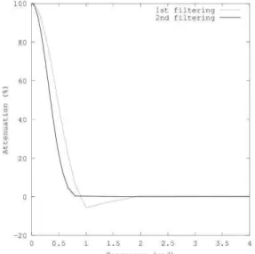
For cross-correlation analysis, the original SL time series was broken down into annual time series and then re-sampled every 6 hours, thus making the SSH and NCEP/NCAR wind time series compatible. The trend obtained by linear regression was removed. Then another Lanczos-square filtering was carried out, with a 36-hour window - similar to the other, 40-hour, filtering already mentioned. This new window was also capable of removing almost all the diurnal and semi-diurnal frequencies (Fig. 2). Finally, the lag correlation between wind speed and SSH was estimated for each year, as well as the confidence level.

Fig. 2.SSH response curve to Lanczos filtering. The black curve represents the results after the double filtering (41 weights). The two lines represent the results after first and second filtering.

SST and AT Climatology

SST and AT climatology were obtained by, first, computing the average AT for each month of the time series and then estimating the average for each month of the year. After removing the monthly means from the monthly time series, the resulting anomaly time series underwent a low-pass filtering process for interannual frequencies (TRENBERTH, 1984).

The temperature climatology was also estimated through the best fit for a cosine function, in a least square approach, given by:

T=Tm+Acos (ωt+φ) (1)

where T is the temperature (for both AT and SST), Tm is the temperature average for the year, A is the amplitude of the seasonal cycle, ω is the annual frequency and φ the phase. Before computing A and φ, the trend was removed from both time series.

Monthly means of along and cross shore winds from NCEP/NCAR were also subjected to the same filtering process and the correlation coefficients between temperature and winds were computed. The correlation coefficients between Nino 3.4 and temperature anomalies were also estimated. The Nino 3.4 index was obtained from the NOAA/CPC website. The definition of the El Nino phenomenon and a discussion of its indexes can be found in Trenberth (1996; 1997).

AT and SST trends were estimated for both the raw, monthly and monthly anomalies time series using a simple linear regression. The results are presented in the next section.

SST and AT subinertial variability

Differently from the previous analyses, the subinertial variability of AT was estimated through the time series for each year separately. The filtering process consisted of removing the linear trend and then filtering the time series using a cosine squared filter with a 48-hour window. Along and cross-shore winds from NCEP/NCAR, sampled every 6 hours, underwent the same process and were interpolated at the same frequency as the AT data to keep them compatible.

R

SL Trend Analysis

Results indicate a SL rise for the first period (1978-1983), followed by a rising, but decelerating pattern during the second period (1987-1993) and a sea level decrease during the third period (1994-2000). This pattern might be linked to the lunar nodal cycle of 18.6 years. However, due to the data gap in the SL series between 1984 to 1986, this assessment cannot be further explored in this work. Results for each period are shown in Table 1.

Table 1. SL trends (mm/year) estimates.

SL results

(mm/year) 1978-1983 1987-1993 1994-2000 Mean Trend for

raw data 13.0 4.0 -10.0 2.3 Trend for

filtered data 13.0 4.0 -15.0 0.7 Tidal Energy Attenuation

diurnal and semidiurnal tidal oscillations were significantly attenuated, as compared to the original signal. For other frequencies with periods between 3 and 20 days (i.e., frequencies from 0.333 to 0.05 cpd), the energy attenuation ranges, respectively, from 47% to 1.4%. As Figure 2 shows, almost all the diurnal and semidiurnal frequencies were removed after the filtering process.

Correlations between MSL and Wind Speed

Figure 3 shows the maximum lag correlation coefficients between mean sea level (MSL) and along-shelf and cross-along-shelf wind for each year of the series and their respective time lags. Results showed a high level of statistical reliability between MSL and the alongshore wind. This indicates that the MSL and the along-shelf wind speed are correlated at about 0.6 for a 99% confidence level (see Figure 3). These results seem to be explained by local wind forcing with simple Ekman dynamics. It is shown that about 40% of the variance of the series can be explained in terms of the local wind, as the correlation coefficients are close to 0.6. Over the 20 years of data used for cross-correlation analysis, only in five of them were the MSL and along-shelf wind in phase. For the rest of the series, results indicated a 6-hour delay, with wind leading MSL variations on subinertial frequencies. On the other hand, there was no significant correlation between the cross-shelf wind and MSL (see Figure 3).

Fig. 3. Maximum correlation coefficients between MSL and alongshelf wind and cross-shelf wind (solid and dashed lines, respectively). The gray solid lines show the 95% and 99% confidence level.

Air and Sea Surface Temperature Analysis

Temperature trends showed a considerable increase for the both AT and SST. For AT, the linear

increase was about 0.087°C/year for the raw series and 0.085°C/year for the monthly mean series. For SST, the linear coefficients were 0.047°C/year and 0.046°C/year, for the raw and monthly time series, respectively.

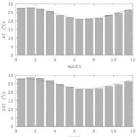
The monthly climatology for both AT and SST are shown in Figure 4 and present the highest value in February, 27.79°C for AT and 28.59°C for SST, the lowest occurring in July, with 21.12°C for AT and 21.91°C for SST. The other method for estimating the seasonal cycle (Equation 1) resulted in the values presented in Table 2 and shown in Figure 4.

Fig. 4. Climatology for AT (top panel) and SST (bottom panel). The solid lines show the results obtained with Equation 1 using the parameters of Table 2.

Air and Sea Surface Temperature Correlation Coefficients

Several lag correlation coefficients were computed for the temperature time-series. Correlation coefficients between AT and SST were, for the raw time series, of 0.82 which, when the trend and seasonal cycle were removed, dropped to 0.56, both cases in phase and with above 99% of statistical confidence. Filtering the anomalous time series for subinertial frequency, the correlation coefficient reached 0.67, above 99% of confidence, but with AT leading SST by about 6 hours. For the anomalous monthly time series, the maximum correlation coefficient was in phase and reached 0.76, for the same confidence level.

Nino3.4 leading to 20 months with temperature leading. For AT, the maximum value was obtained with Nino3. 4 leading for one month, reaching 0.53. For SST, the maximum lag correlation is 0.35, with Nino3.4 leading by 3 months. AT maximum lag correlation with Nino 3.4 was slightly below the 95% confidence level while for SST it was not statistically significant.

Neither of the maximum lag correlations between temperature and wind, whether along or cross shelf, were statistically significant when filtered for interannual frequencies, as described for Nino3.4 correlations. At subinertial frequencies, the maximum lag correlation between wind and temperature was not statistically significant either.

Table 2. Parameters obtained for Equation (1) for AT and SST.

Variables mean value amplitude phase

AT 24.31°C 3.33°C 34.5 days

SST 24.91°C 2.85°C 34.5 days

D

This study used a historical dataset acquired at the IOUSP station to assess the behavior of the sea level and temperature in the coastal region of Ubatuba on the northern coast of São Paulo state. In Brazil, long term records of oceanographic parameters are rare and, therefore, the datasets used in this study are very important for contributions to studies of sea level and temperature. However, there is a lack in the geodetic monitoring of this tide gauge data and it is therefore extremely important to provide reliable data. The partnership between research groups and the agencies (e.g., universities and government institutions) responsible for data acquisition and geodetic monitoring can provide a significant improvement in the collection of such data.

Regarding the filtering process, a considerable amount of recorded data relating to the third period was removed, seeing that gaps were more common between 1994 and 2000. Therefore, the results obtained for the SL rise from the raw data set seemed more appropriate and, were, in fact, closer to the values commonly observed worldwide. As can be seen in Table I, the first two periods, which contained very few data gaps, gave similar values for the raw and filtered time series.

Both raw and filtered SL trends were positive for the periods 1978 – 1983 (13 mm/year) and 1987 – 1993 (4 mm/year). For the third period, 1994 – 2000, there was a difference between the raw and filtered SL trends, - 10 mm/year and – 15 mm/year,

respectively, which could have been influenced by sparser data sampling during this period and its effects in abruptly increasing the lengths of the gaps during the filtering process. The overall SL pattern might be linked to the lunar nodal cycle of 18.6 years. However, due to the data gap in the SL series between 1984 to 1986, this assessment cannot be further investigated in this study.

It should also be noted that 7 years of data analyses could lead to erroneous conclusions and it is highly recommended that longer periods of analyses be used to assess low-frequency SL variations. After the application of the Lanczos cosine filter, the attenuation of semi-diurnal and diurnal frequencies was virtually achieved. As shown in Figure 2, there was a respective reduction of almost 99% and 97%, for semi-diurnal and diurnal components. At frequencies below 0.6 cpd, it was not possible to find a peak in any specific frequency. However, the subinertial band is clearly more energetic than the others.

The cross-correlation between SL and along-shelf and cross-along-shelf wind showed different behaviors. The maximum lag correlation coefficients showed a correlation of the order of 0.6 between along-shelf wind and SL with a statistical confidence of at least 99%. On the other hand, correlations between SL and cross-shelf wind were much lower, even below 95% statistical confidence levels during most of the time. Over the 21 years of analysis, the statistical threshold was observed only in three years (1983, 1991 and 1998). Thus, these results suggested that there is virtually no significant correlation between the cross-shelf wind and the subinertial SL in the study area (Fig. 3). These results are in agreement with those of other studies such as Castro and Lee's (1995).

Regarding recommendations for future study, better quality control of data, especially those of geodetic monitoring, is suggested. As for wind data, the installation of a network of meteorological and oceanographic stations in coastal and oceanic regions adjacent to the study area is recommended, as well as the use of other grid points of the global model.

Temperature trends were positive for both AT and SST. The higher values of temperature increase for AT are, probably, due to the higher heat retention capacity of the water.

whether this is an important topic of study for the region.

A

The authors thank Prof. Claudio Neves (COPPE-UFRJ) and the referees for their invaluable comments to prepare this work. Also, to CAPES (institution linked to the Brazilian Ministry of Education), Redelitoral Project (www.redelitoral.ita.br), FAPESP(Project2010/05124-1) for the financial supports and CNPq, for the Scientific Initiation scholarship.

R

ANDRADE, K. M.; CAVALCANTI, I. F. A. Climatologia dos sistemas frontais e padrões de comportamento para o verão na América do Sul. In: CONGRESSO BRASILEIRO DE METEOROLOGIA, 13., 2004, Fortaleza. Anais. Fortaleza: SBMet, 2004. 1 CD-ROM (INPE-12090-PRE/7436).

CAMPOS, E. J. D.; LENTINI, C. D.; MILLER, J. L.; PIOLA, A. R. Interannual variability of the sea surface temperature in the South Brazil Bight. Geophys. Res. Lett., v. 26, n. 14, p. 2061-2064, 1999.

CASTRO, B. M.; LEE, T. Wind-forced sea level variability on the Southeast Brazilian shelf. J. Geophys. Res., v.100, n. 8, p.16045-16056, 2012.

CASTRO, B. M.; LORENZZETTI, J. A.; SILVEIRA, I. C. A.; MIRANDA, L. B. Estrutura termohalina e circulação na região entre Cabo de São Tomé (RJ) e o Chuí (RS). In: ROSSI WONGTSCHOWSKI, C. L. B.; MADUREIRA, L. S. P. (Orgs.). O ambiente oceanográfico da plataforma continental e do talude na região sudeste-sul do Brasil. São Paulo: EDUSP, 2006. p. 11-120.

CSANADY, G. T. Circulation induced by river inflow in well-mixed water over a sloping continental shelf. J. Phys. oceanogr., v. 14, p. 1703-1711, 1984.

DEAN, R. G.; HOUSTON, J. R. Recent sea level trends and accelerations: comparison of tide gauge and satellite results. Coastal Eng., v. 75, p. 4-9, 2013.

DENNIS, K. C., SCHNACK, E. J., MOUZO, F. H.; ORONA, C. R. Sea-level rise and Argentina: potential impacts and consequences. J. Coastal Res., n. 14, sp. iss., p. 205-223, 1995.

DOTTORI, M.; CASTRO, B. M. The response of the São Paulo Continental Shelf, Brazil, to synoptic winds. ocean Dyn., v. 59, n. 4, p. 603-614, 2009.

HARARI, J.; FRANÇA, C. A. S.; CAMARGO, R. Variabilidade de longo termo de componentes de maré e do nível médio do mar na costa brasileira. 2008. Disponível em: http://migre.me/3aOax. Acesso em: 10 jan. 2010.

HEBERGER, M.; COOLEY, HERRERA, P.; GLEICK, P.H.; MOORE, E. The Impacts of sea-level rise on the California coast. California: California Climate Change Center, 2009. 101 p. Disponível em:

http://www.pacinst.org/wp-content/uploads/2013/02/report16.pdf. Acesso em: 01 jul. 2012.

KALNAY, E.; KANAMITSU, M.; KISTLER, R.;COLLINS, W.; DEAVEN, D.; GANDIN, L.; IREDELL, M.; SAHA, S.; WHITE, G.; WOOLLEN, J.; ZHU, Y.; LEETMAA, A.; REYNOLDS, R.; CHELLIAH, M.; EBISUZAKI, W.; HIGGINS, W.; JANOWIAK, J.; MO, K. C.; ROPELEWSKI, C.; WANG, J.; JENNE, R.; JOSEPH, D. The NCEP/NCAR 40-Year Reanalysis Project. Bull. Am. Meteorol. Soc., v. 77, n. 3, p. 437-477, 1996. LANCZOS, C. Applied analysis. Englewood Cliffs:

Prentice-Hall, 1956. 539 p.

LENTINI, C. A. D.; PODESTÁ, G. P.; CAMPOS, E. J. D.; OLSON, D. B. Sea surface temperature anomalies on the Western South Atlantic from 1982 to 1994. Cont. Shelf Res., v. 21, n.1, p. 89-112, 2001.

MONTEIRO, C. A. F. A dinâmica climática e as chuvas no Estado de São Paulo: estudo geográfico sob a forma de atlas. São Paulo: Instituto de Geografia/USP, 1973. 130p.

NEVES, C. F.; MUEHE, D. Vulnerabilidade, impactos e adaptação a mudanças do clima: a zona costeira. Parcerias Estratégicas, n.27, p. 217-297, 2008. [Mudança do clima no Brasil: vulnerabilidade, impactos e adaptação]. Disponível em: http://www.cgee.org.br/parcerias/p27.php. Acesso em: 01 jun. 2009.

SALLENGER JR., A. H.; DORAN, K. S.; HOWD, P. A. Hotspot of accelerated sea-level rise on the Atlantic coast of North America. Nature Climate Change, Vol. 2: 884 – 888. Disponível em http://www.nature.com/nclimate/journal/v2/n12/pdf/ncl imate1597.pdf . Acesso em 03 mar 2013.

SANT’ANNA NETO, J. L. Ritmo climático e a gênese das chuvas na Zona Costeira Paulista. In: ENCUENTRO DE GEÓGRAFOS DE AMÉRICA LATINA, 3., Toluca, 1991. Memórias. Tolua: Universid Nacional Autónoma de Mexico (UNAM), 1991. v.2, p.49-66.

SANT’ANNA NETO, J. L. Tipologia dos sistemas naturais costeiros do Estado de São Paulo. Rev. Geogr., n. 12, p. 47-86, 1993.

TRENBERTH, K. E. Signal versus noise in the Southern Oscillation. Mon. Weather Rev., v. 112, n. 2, p. 326-332, 1984.

TRENBERTH, K. E. El Nino definition. CLIVARExch., v. 1, n. 3, p. 6-8, 1996. Disponível em: http://eprints.soton.ac.uk/19273/1/ex3.pdf. Acesso em: 01 jul. 2009.

TRENBERTH, K. E. The definition of El Nino. Bull. Am. Meteorol. Soc., v. 78, p. 2771-2777, 1997.