Article
0103 - 5053 $6.00+0.00*e-mail: [email protected]
Multivariate Calibration Transfer Employing Variable Selection and Subagging
Marcelo N. Martins,a Roberto K. H. Galvão*,a and Maria Fernanda Pimentelb
aInstituto Tecnológico de Aeronáutica, Divisão de Engenharia Eletrônica,
12228-900 São José dos Campos-SP, Brazil
bDepartamento de Engenharia Química, Universidade Federal de Pernambuco,
50740-521 Recife-PE, Brazil
Neste artigo, é proposta uma nova técnica para transferência de calibração, que combina o Algoritmo das Projeções Sucessivas (APS) para seleção de variáveis robustas com a técnica de sub-amostragem e agregação de modelos conhecida como subagging. A técnica proposta tem por objetivo construir modelos de Regressão Linear Múltipla (RLM) que sejam robustos com respeito a diferenças na resposta instrumental de dois espectrômetros (primário e secundário). Para isso, um pequeno conjunto de amostras de transferência, com espectros adquiridos no instrumento secundário, é empregado para guiar o procedimento de seleção de variáveis. A eiciência da técnica proposta é demonstrada em um estudo de caso envolvendo a determinação por FT-IR da massa especíica e duas temperaturas de destilação (T10%, T90%) em amostras de gasolina e a determinação por NIR de umidade em amostras de milho. Em termos do erro quadrático médio de predição no espectrômetro secundário, os modelos RLM gerados pela abordagem APS-subagging forneceram resultados melhores que os obtidos por Mínimos Quadrados Parciais empregando Padronização Direta por Partes. Em particular, o uso de subagging resultou em uma redução mais sistemática do erro de predição com a inclusão progressiva de amostras de transferência.
This paper proposes a new technique for calibration transfer, which combines the Successive Projections Algorithm (SPA) for robust variable selection with the subsampling and model aggregation technique known as subagging. The proposed technique is aimed at building Multiple Linear Regression (MLR) models that are robust with respect to differences in the instrumental response of two spectrometers (primary and secondary). For this purpose, a small set of transfer samples with spectra acquired at the secondary instrument is employed to guide the variable selection procedure. The eficiency of the proposed technique is demonstrated in a case study concerning the FT-IR determination of speciic mass and two distillation temperatures (T10%, T90%) for gasoline samples and the NIR determination of moisture in corn samples. In terms of the root-mean-square error of prediction at the secondary spectrometer, the MLR models obtained according to the SPA-subagging approach provided better results in comparison with Partial Least Squares employing Piecewise Direct Standardization. In particular, the use of subagging resulted in a more systematic reduction in the prediction error with the progressive inclusion of transfer samples.
Keywords: multivariate calibration, calibration transfer, variable selection, successive projections algorithm, subagging
Introduction
In a wide sense, the term Calibration Transfer concerns a body of methods aimed at compensating for changes in experimental conditions that would compromise the prediction accuracy and reliability of a multivariate model. Such changes may refer to physical/
acquisition is not the same as the one used for building the calibration model.1
The methods for calibration transfer can be divided in two basic approaches, namely: (i) Standardization of the model coeficients, instrumental responses, or predicted values. Examples of this approach include the univariate standardization method of Shenk and Westerhaus,2 Slope/ Bias Correction (SBC),3 Direct Standardization (DS) and Piecewise Direct Standardization (PDS),4 among many others. (ii) Enhancement of model robustness. This approach encompasses the development of global models by inclusion of all the relevant sources of variation in the calibration data set,5 as well as the use of pre-processing techniques to reduce the data variability that is not correlated to the y-property of interest. Examples of such techniques include baseline correction procedures,6 Multiplicative Signal Correction (MSC),7 Finite Impulse Response (FIR) ilters,8 Orthogonal Signal Correction (OSC),9 wavelet decompositions,10 Transfer by Orthogonal Projections (TOP)11 and variable selection algorithms.12,13
In addition, the methods can be divided into those based on data acquired under the two experimental conditions of interest (transfer data set) and those based solely on a single calibration data set. The use of transfer data provides valuable information concerning differences in the instrumental response caused by the changes in experimental conditions. However, the acquisition of such data can be cumbersome if, for instance, one desires to transfer the calibration between two instruments located in different laboratories.
Within the framework of variable selection for enhancement of model robustness, a recently proposed strategy involves the use of the Successive Projections Algorithm (SPA).13 This algorithm was originally proposed for the minimization of collinearity problems in Multiple Linear Regression (MLR).14 Honorato et al.13 adapted SPA to select variables that convey information concerning the property of interest and are robust with respect to the differences between two instruments. The proposed strategy was applied to two calibration transfer problems involving the determination of T90% in gasoline by FT-IR spectrometry and moisture in corn by Near Infrared (NIR) spectrometry. The results were favourably compared to those obtained by a Partial-Least-Squares (PLS) model employing PDS, which is typically used as a benchmark in calibration transfer studies.1 Both SPA and PDS use a transfer data set. However, unlike PDS, SPA does not require the same samples to be measured at both instruments. This can be a signiicant advantage if the instruments are located far apart or if the calibration transfer is aimed at compensating changes in the response of a single instrument over time.
This paper proposes an improvement on the selection of robust variables by SPA based on a technique known as Subagging.15 Subagging, which stands for Sub-sampling and Aggregating, generates an ensemble model from the combination of different models obtained by resampling the available data set. In a single-instrument calibration scenario, the use of subagging has been shown to provide considerable improvements on the prediction performance of MLR-SPA models.16 In view of such indings, the present paper investigates whether similar improvements can be obtained in the calibration transfer context.
Two data sets are employed to validate the proposed SPA-Subagging method. The first data set consists of gasoline samples with FT-IR spectra from two spectrometers, as well as reference values of speciic mass and two distillation temperatures (T10% and T90%). These parameters are routinely used to monitor fuel quality, as well as to check conformity with standards issued by regulatory agencies. The second data set consists of corn samples with NIR spectra from two spectrometers and reference values of moisture. In both examples, the results are compared with those obtained by PLS models with the use of PDS.
Background and theory
Robust variable selection by SPA
In what follows, the instrumental response data available for calibration are assumed to be disposed in a matrix Xcal of dimensions (Ncal× K) such that the kth variable xk is associated to the kth column vector x
k∈ℜ
Ncal. The basic
SPA formulation comprises two phases. The first phase consists of projection operations involving the columns of the Xcal matrix. These projections are used to deine K chains of M variables each, where M = min{Ncal− 1, K} is the maximum number of variables that can be included in an MLR model with intercept term. Each chain starts with one of the variables under consideration and is successively augmented with additional variables chosen in order to display the least collinearity with the previous ones, as described in earlier papers.14,17 The notation {SEL(1, k), SEL(2, k), …, SEL(M, k)} is used to denote the index set of variables belonging to the chain initialized with xk (that is, SEL(1, k) = k).
an MLR model, which is then applied to a separate set of Nval validation samples not included in the regression. The best subset is selected according to the minimum of the root-mean-square error of validation (RMSEV) deined as
(1)
where yval,n and ^
yval,n are the reference and predicted values of the parameter under consideration for the nth validation sample.
In the context of calibration transfer,13 a modiication was proposed in order to select variables with greater robustness with respect to the differences between two given instruments (termed primary and secondary). For this purpose, a transfer data set of Ntransf samples with spectra acquired at the secondary instrument was assumed to be available. The RMSEV metric employed in Phase 2 of SPA was then replaced with the following performance index:
E = 0.5 (RMSEV + RMSET) (2)
In this equation, RMSET is the root-mean-square error of prediction for the transfer data set, deined as
(3)
where ytransf,n and ^
ytransf,n are the reference and predicted values of the parameter under consideration for the nth transfer sample. It is worth noting that E evaluates not only the predictive ability of the model (assessed by RMSEV) but also its robustness (assessed by RMSET).
Subagging
The term Bagging (Bootstraping18 and Aggregating) refers to a class of techniques in which an ensemble model is obtained by combining different models generated by randomly resampling the available data set.19-23 In the most usual approach, the resampling process is applied to the original set of N objects in order to generate different calibration sets with the same number N of objects (including possible repetitions of the same object). Each of these sets is used to obtain a model by following usual multivariate calibration methods. Finally, the resulting models are combined according to some suitable ensembling procedure. In the case of MLR models, such a combination amounts to averaging the regression coeficients.20
As demonstrated by Breiman22 this procedure can lead to signiicant improvements in prediction ability, mainly related to reductions in the variance of the predictions.
In particular, variable selection procedures for MLR may beneit from a smoothing effect in the regression coeficients induced by bagging.23 In fact, since different variables can be selected in the course of the resampling iterations, each variable may have a non-zero weight in the inal ensemble model, instead of just being included in or excluded from the regression. It is interesting to notice that the number of variables selected for each individual MLR model must be smaller or equal to the number of calibration objects in order to avoid ill-conditioning problems. However, as a result of the model averaging process, the ensemble model may have more variables than the number of objects available for calibration.
More recently, a method termed subagging (Subsampling and Aggregating) was proposed as an alternative to bagging.15 In this method, each individual model is constructed on the basis of a reduced number of Ncal < N objects randomly extracted, without replacement, from the available pool of N objects. The resulting models are then combined as discussed above. Such a procedure has computational advantages with respect to bagging because the calibration of each individual model is faster if fewer objects (Ncal instead of N) are employed in the regression. For example, in an MLR problem involving 20 variables, reducing the number of calibration objects from N = 80 to Ncal = 50 decreases the computational time by approximately 25%. Such a result was obtained by using a Core 2 Duo processor running Matlab 6.5.
A subagging strategy was proposed elsewhere16 to improve the accuracy of multivariate calibration models in spectrometric analysis. More speciically, subagging was applied to PLS models, as well as to MLR models obtained by using variable selection algorithms, namely SPA and a genetic algorithm (GA). In the proposed strategy, different models were obtained by randomly dividing the available pool of modelling samples into calibration and validation sets. The validation set was used to guide the selection of variables in SPA and GA. A case study involving the NIR determination of four diesel quality parameters (speciic mass, sulphur content, and two distillation temperatures (T10% and T90%) was presented to demonstrate the effectiveness of the subagging approach. In the particular case of SPA, improvements of up to 33% were obtained in the prediction accuracy of the resulting MLR model.
Proposed method for calibration transfer
sets of Ncal calibration objects and Nval validation objects such that Ncal + Nval = N. Moreover, it is assumed that Ntransf samples, with spectra acquired at the secondary instrument, are available for calibration transfer. The spectral measurements of such samples do not necessarily need to be repeated at the primary instrument.
Figure 1 depicts the steps involved in the proposed subagging procedure. Given two sets of calibration and validation data, obtained by splitting the overall set of modelling data, and a transfer data set, the SPA formulation for robust variable selection is applied to generate an MLR model. After this procedure has been repeated a number of times, the resulting models are averaged in order to generate an ensemble model. It is worth noting that the transfer data set remains the same in all iterations.
In a recent paper,16 the incremental improvements in prediction accuracy for MLR-SPA were found to be minor after 30 subagging iterations. Therefore, this number will be adopted in the present work.
Experimental
Data sets
The same data sets employed in our previous studies13 were adopted in the present work.
The irst data set comprises 103 gasoline samples collected from gas stations in the Brazilian states of Pernambuco and Alagoas. Our previous work13 was concerned with the determination of the distillation temperature at which 90% of the sample has evaporated (T90%). In the present work, the speciic mass (SM) and the T10% distillation temperature were also considered.
The primary and secondary instruments were both FT-IR Perkin Elmer Spectrum GX spectrometers. The absorbance spectra were acquired with a spectral resolution of 4 cm-1 in the range 2500-15400 nm. Additional details concerning the spectral acquisition process are given in reference 13.
The second data set comprises NIR relectance spectra and moisture content from 80 corn samples (publicly available at www.eigenvector.com/Data/Corn/). The spectra were acquired in the range 1100-1498 nm at instruments m5 and mp5 of this data set, which were adopted as the primary and secondary instruments for the present investigation.
To circumvent the problem of systematic baseline variations, first-derivative spectra were employed by using a Savitzky-Golay ilter with a 2nd-order polynomial and a 21-point window.6 The original and derivative spectra for the diesel and corn samples are included in the Supplementary Information.
The data sets were divided into calibration, validation and prediction sets on the basis of a preliminary PLS analysis13 employing full cross-validation. The gasoline data set was divided into 63 calibration, 20 validation and 20 prediction samples, whereas the corn data set was divided into 40 calibration, 20 validation and 20 prediction samples.
The validation set was employed in the choice of an appropriate number of latent variables in PLS and to guide the selection of variables in SPA. For the subagging study, the calibration and validation sets were merged into a single modelling set, which was subjected to the subsampling procedure described in the proposed method for calibration transfer. In all cases, the prediction set was employed to compare the performance of the PLS and MLR models in terms of the root-mean-square error of prediction (RMSEP).
The transfer samples were selected from the calibration set according to the classical Kennard-Stone algorithm.1,24 This algorithm is aimed at covering the sample space in a uniform manner by maximizing the Euclidean distances between the spectra of the selected samples. The effect of varying the number Ntrans of transfer samples from 2 to 15 was investigated.
Modelling procedures
All calculations were carried out by using lab-made programs implemented in the Matlab 6.5 software. The number of latent variables in the PLS model was determined on the basis of the error in the validation set by using the
F-test criterion of Haaland and Thomas with α = 0.25 as suggested elsewhere.25,26 The PDS window was varied from 3 to 15 and the best and worst results for each number of transfer samples were noted.
In the subagging procedure, the resampling values were Ncal = 50, Nval = 33 for the gasoline set and Ncal = 36, Nval = 24 for the corn set. Such numbers follow a proportion suggested elsewhere.16 The MLR models obtained by using subagging in conjunction with SPA will be termed MLR-SPASubag.
In the discussion of the results, the notation RMSEPAB will be used to represent the RMSEP value obtained at instrument B by using the model calibrated for instrument A. If some transfer procedure is employed, the notation RMSEPA-TB will be adopted. The primary and secondary instruments will be represented by letters P and S, respectively.
Results and Discussion
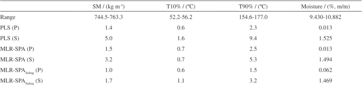
Table 1 presents the RMSEP values obtained without the use of calibration transfer techniques at the primary and secondary instruments. As can be seen, with the
exception of the T10% case for MLR-SPA, the prediction performance of all models is substantially deteriorated when applied to data acquired at the secondary instrument, which justiies the use of calibration transfer.
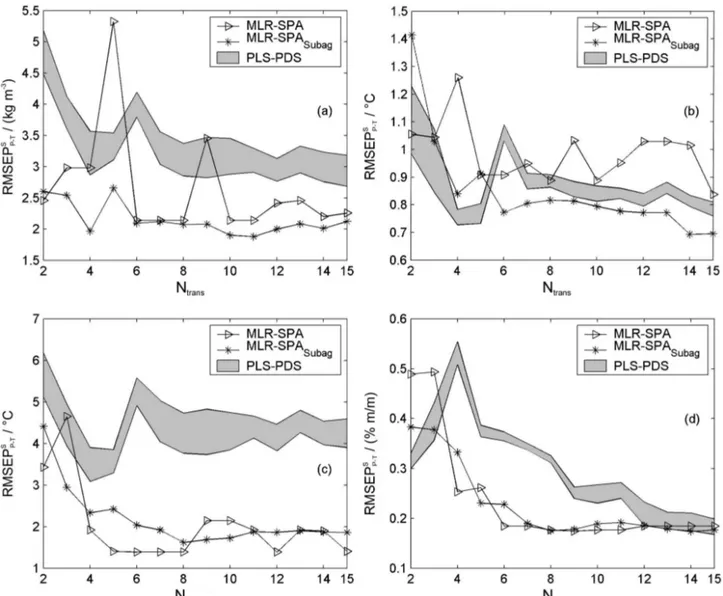
Figure 2 presents the curves of RMSEPP-TS as a function of the number of transfer samples (Ntrans) for the three calibration transfer techniques under consideration. For PLS-PDS, the boundaries of the shaded area correspond to the best and worst results obtained by varying the window size. By contrasting the RMSEP values in this igure with those presented in Table 1, it can be seen that the use of calibration transfer techniques did improve the prediction results obtained at the secondary instrument. As compared to the best results of PLS-PDS, MLR-SPASubag is considerably better for SM and T90%, slightly better for moisture and similar for T10%. In the moisture case, it is worth noting that PLS-PDS only achieves the performance of MLR-SPASubag if a suficiently large number of transfer samples is employed (Ntrans≥ 12). Another positive aspect of MLR-SPASubag is a more systematic tendency of reduction in RMSEPP-TS with the number of transfer samples, in comparison with the behaviour observed for MLR-SPA and PDS-PLS.
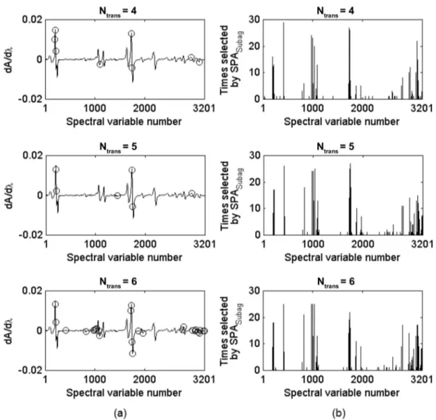
The advantage of SPASubag over SPA can be better understood by analyzing Figure 3, which depicts the variables selected for T10% with the use of transfer samples. As can be seen in Figure 3a, the inclusion of each additional transfer sample may cause a considerable change in the variables selected by SPA. In some cases, such a change may have detrimental effects, which are relected in a large local increase in the curve of RMSEPP-TSversus Ntrans. Therefore, the choice of Ntrans may be a critical task for the performance of SPA in the context of calibration transfer. On the other hand, in SPASubag this problem is attenuated by the averaging effect of subagging, which can be explained by considering the histograms in Figure 3b. The relative frequency of selection for each variable
Table 1. RMSEPPP and RMSEP P
S values obtained with the models developed for the primary instrument. In this case, no calibration transfer procedures
were employed
SM / (kg m-3) T10% / (ºC) T90% / (ºC) Moisture / (%, m/m)
Range 744.5-763.3 52.2-56.2 154.6-177.0 9.430-10.882
PLS (P) 1.4 0.6 2.3 0.013
PLS (S) 5.0 1.6 9.4 1.525
MLR-SPA (P) 1.5 0.7 2.5 0.013
MLR-SPA (S) 3.2 0.7 5.3 1.494
MLR-SPASubag (P) 1.0 0.6 1.5 0.062
MLR-SPASubag (S) 1.7 1.1 3.2 1.469
(number of times that the variable was selected divided by a total of 30 subagging iterations) may be regarded as the weight assigned to this variable in the inal ensemble model. As Ntrans is increased in SPASubag, the weight for each variable can be modiied in a gradual manner, in comparison with the binary (include/exclude) outcome of a standard variable selection procedure.
Conclusions
This paper proposed a new technique for calibration transfer, which combines the use of robust variable selection by SPA with the subsampling and model aggregation technique known as subagging. The proposed approach is aimed at building MLR models that are robust with respect to the differences between two instruments.
The results obtained with both FT-IR and NIR data sets demonstrate that subagging does provide systematic
improvements on the SPA-based strategy for variable selection in calibration transfer. In particular, the use of subagging resulted in a more systematic reduction in the prediction error of the secondary instrument with the successive inclusion of transfer samples. Such a systematic behaviour, associated to the smoothing effect of the model averaging procedure in subagging, is important to facilitate the choice of an adequate number of transfer samples.
In comparison with the classical PDS-PLS standardization approach, the proposed SPA-Subagging strategy provided better transfer results in all cases considered in the study. In addition, it should be emphasized that the SPA-Subagging does not require the same samples to be measured at the primary and secondary instruments. Although such a possibility was not exploited in the present work, it could be an important advantage in situations where the storage and/or physical transportation of transfer samples proves to be impractical.
Figure 2. RMSEPP-TS values as a function of the number N
Figure 3. Variables selected for the determination of T10% by (a) SPA and (b) SPASubag for different numbers of transfer samples. In the SPASubag case, the histograms indicate the number of times that each variable was selected in the course of the subagging iterations.
Acknowledgments
The support of CNPq (MSc scholarship, research fellowships and Universal grant 475204/2004-2), FAPESP (doctorate scholarship 05/04400-7), CAPES (PROCAD grant 0081/05-1) and FINEP-CTPETRO Research Program is gratefully acknowledged. The authors wish to thank Dr. Fernanda Araújo Honorato for collaborating in the acquisition of the gasoline spectra. The authors are also indebted to Prof. Mário César Ugulino de Araújo
(LAQA/UFPB) for granting access to the secondary FT-IR
spectrometer.
Supplementary Information
Supplementary data are available free of charge at http://jbcs.sbq.org.br, as PDF ile.
References
1. Feudale, R. N.; Woody, N. A.; Tan, H.; Myles, A. J.; Brown, S. D.; Ferré, J.; Chemom. Intell. Lab. Syst.2002, 64, 181. 2. Shenk, J. S.; Westerhaus, M. O.; Templeton Jr., W. C.; Crop
Sci. 1985, 25, 159.
3. Bouveresse, E.; Hartmann, C.; Massart, D. L.; Last, I. R.; Prebble, K. A.; Anal. Chem. 1996, 68, 982.
4. Wang, Y.; Veltkamp, D. J.; Kowalski, B. R.; Anal. Chem. 1991, 63, 2750.
5. Despagne, F.; Massart, D. L.; Chabot, P.; Anal. Chem. 2000, 72, 1657.
6. Beebe, K. R.; Pell, R. J.; Seasholtz, B.; Chemometrics: A Practical Guide, Wiley: New York, 1998.
8. Blank, T. B.; Sum, S. T.; Brown, S. D.; Anal. Chem. 1996, 68, 2987.
9. Pierna, J. A. F.; Massart, D. L.; de Noord, O. E.; Ricoux, P.; Chemom. Intell. Lab. Syst. 2001, 55, 101.
10. Yoon, J.; Lee, B.; Han, C.; Chemom. Intell. Lab. Syst. 2002, 64, 1.
11. Andrew, A.; Fearn, T.; Chemom. Intell. Lab. Syst. 2004, 72, 51. 12. Swierenga, H.; Haanstra, W. G.; de Weijer, A. P.; Buydens, L.
M. C.; Appl. Spectrosc. 1998, 52, 7.
13. Honorato, F. A.; Galvão, R. K. H.; Pimentel, M. F.; Barros Neto, B.; Araujo, M. C. U.; Carvalho, F. R.; Chemom. Intell. Lab. Syst. 2005, 76, 65.
14. Araujo, M. C. U.; Saldanha, T. C. B.; Galvão, R. K. H.; Yoneyama, T.; Chame, H. C.; Visani, V.; Chemom. Intell. Lab. Syst. 2001, 57, 65.
15. Bühlmann, P.; Yu, B.; Ann. Stat. 2002, 30, 927.
16. Galvão, R. K. H.; Araujo, M. C. U.; Martins, M. N.; José, G. E.; Pontes, M. J. C.; Silva, E. C.; Saldanha, T. C. B.; Chemom. Intell. Lab. Syst. 2006, 81, 60.
17. Galvão, R. K. H.; Pimentel, M. F.; Araujo, M. C. U.; Yoneyama, T.; Visani, V.; Anal. Chim. Acta 2001, 443, 107.
18. Efron, B.; Tibshirani, R. J.; An Introduction to the Bootstrap, CRC Press: Boca Raton, 1993.
19. Opitz, D. W.; Maclin, R. J.; J. Artif. Intell. Res. 1999, 11, 169. 20. Skurichina, M.; Duin, R. P. W.; Pattern Recognition 1998, 31,
909.
21. Martin, E. B.; Morris, A. J. In Statistics and Neural Networks-Advances at the Interface; Kay, J. W.; Titterington, D. M., eds.; Oxford University Press: Oxford, 1999, pp. 195-258. 22. Breiman, L.; Mach. Learn. 1996, 24, 123.
23. Breiman, L.; Mach. Learn. 1996, 24, 41.
24. Kennard, R. W.; Stone, L. A.; Technometrics1969, 11, 137. 25. Haaland, D. M.; Thomas, E. V.; Anal. Chem. 1988, 60, 1193. 26. Li, B. X.; Wang, D. M.; Xu, C. L.; Zhang, Z. J.; Microchim.
Acta2005, 149, 205.
Received: February 10, 2009
Web Release Date: October 23, 2009
Supplementary Information
0103 - 5053 $6.00+0.00
*e-mail: [email protected]
Multivariate Calibration Transfer Employing Variable Selection and Subagging
Marcelo N. Martins,a Roberto K. H. Galvão*,a and Maria Fernanda Pimentelb
aInstituto Tecnológico de Aeronáutica, Divisão de Engenharia Eletrônica,
12228-900 São José dos Campos-SP, Brazil
bDepartamento de Engenharia Química, Universidade Federal de Pernambuco,
50740-521 Recife-PE, Brazil
Figure S1. FT-IR spectra of the gasoline samples acquired at the (a) primary and (b) secondary instruments.
Figure S2. NIR spectra of the corn samples acquired at the (a) primary and (b) secondary instruments.
Figure S3. Derivative spectra of the gasoline samples. (a) Primary, (b) secondary and (c) differences between the two instruments.