A proposal for generating gsgp-hard datasets : an introductory research towards gsgp hardness

(1)

i

A Proposal for Generating GSGP-Hard Datasets

Cornelis Marnik Verschoor

An introductory research towards GSGP hardness

Dissertation presented as partial requirement for obtaining

the Master’s degree in Advanced Analytics

(2)

(3)

iii

NOVA Information Management School

Instituto Superior de Estatística e Gestão de Informação

Universidade Nova de Lisboa

A PROPOSAL FOR GENERATING GSGP HARD DATASETS

by

Cornelis Marnik Verschoor

Dissertation report presented as partial requirement for obtaining the Master’s degree in Advanced Analytics

Advisor: Leonardo Vanneschi

(4)

A PROPOSAL FOR GENERATING GSGP HARD DATASETS

Copyright © Cornelis Marnik Verschoor, NOVA Information Management School, NOVA

University of Lisbon.The NOVA Information Management School and the NOVA University of

Lisbon havethe right, perpetual and without geographical boundaries, to file and publish this

dissertation through printed copies reproduced on paper or on digital form, or by any other

means known or that may be invented, and to disseminate through scientific repositories

and admit its copying and distribution for non-commercial, educationalor research purposes,

as long as credit is given to the author and editor.

(5)

Acknowledgements

As to be expected, writing this thesis did not come without its obstacles, robbing me of at least some of my motivation at numerous occasions. Luckily, I’ve found myself surrounded with people who could aid me with their expertise or simply with their presence and support, keeping me on track towards finishing this thesis.

I would first and foremost like to thank professor Leonardo Vanneschi of the In-formation Management School at Universidade Nova de Lisboa. His expertise on the subject of this thesis has been invaluable to me during numerous stages into this re-search. His enthusiasm on the subject gave me a motivational boost after each meeting we had and his willingness to help is admirable and appreciated. Despite his busy schedule, he was always readily available for me whenever I had any questions. This thesis would not have been what it is now without his help.

I would furthermore like to thank my family and friends. Their presence has been of great importance to me throughout my life and during this research. They provided me with constant support, even in the last months when this thesis kept me from giving them the attention they deserve. Besides their support, they also provide me with much needed distraction.

In particular I would like to mention my parents. To thank them for all the things they have done for me in my life so far would require a thesis on itself, therefore I’d like to concretely express my gratitude for the last 2 years. Without them I would not have been able to move to Lisbon, where I attended my master’s degree and was privileged to live in one of Europe’s finest cities (in my humble opinion). Their support and encouragement enabled me to complete this thesis and with it my master’s degree. Maybe even more so, they enabled me to grow as a person.

Thank you

(6)

Abstract

Since its introduction, GSGP has been very successful in optimizing symbolic regres-sion problems. GSGP has shown great convergence ability, as well as generalization ability. Almost without exception, GSGP outperforms GP on real life applications. These results give the impression that almost all symbolic regression problems are easy for GSGP to solve. However, little to no research has been done towards GSGP hardness, while GP hardness has been researched quite extensively already. The lack of real life applications on which GSGP has more difficulty converging than GP creates a paradox: if there are no, or very little, problems that are GSGP hard, no research can be done towards it. In this paper we propose an algorithm that generates and evolves datasets on which GP outperforms GSGP, under the condition that the GP model re-mains as accurate as possible. The algorithm can also be altered so that it produces datasets in which GSGP outperforms GP. This allows for comparing GP hard datasets with GSGP hard datasets. The algorithm has shown to be able to produce favorable datasets for both GP and GSGP using multiple settings for the number of instances and the number of variables. Therefore, the algorithm proposed in this paper breaks the earlier mentioned paradox by producing GSGP hard datasets, thus allowing GSGP hardness to be effectively researched for the first time. Furthermore, tuning the algo-rithm led to some early observations about the relation between dataset composition and GP/GSGP performance. GSGP has difficulty converging when using only 1 de-pendent variable and 1 indede-pendent variable, while it is easy to produce datasets on which GP heavily outperforms GSGP with the same settings. GSGP performs better when more independent variables are added. Furthermore, a big range of the dataset has been shown to be beneficial for GP convergence, while a small range is beneficial for GSGP convergence.

Keywords: Geometric Programming; Geometric Semantic Genetic Programming; Par-ticle Swarm Optimizaion; Multi Objective Optimization; Multi Objective ParPar-ticle Swarm Optimizaion; GP hardness; GSGP hardness

(7)

3 Methodology & Results 9 3.1 Phase I . . . 10 3.1.1 Experimental Setup . . . 11 3.1.2 Results . . . 12 3.1.3 Discussion . . . 13 3.2 Phase II . . . 14 3.2.1 Experimental Setup . . . 14 3.2.2 Results . . . 15 3.2.3 Discussion . . . 18 3.3 Phase III . . . 18 3.3.1 Experimental Setup . . . 19 3.3.2 Results . . . 19 3.3.3 Discussion . . . 23 3.4 Phase IV . . . 24 3.4.1 Experimental Setup . . . 24

(8)

C O N T E N T S 3.4.2 Results . . . 25 3.4.3 Discussion . . . 33 3.5 Phase V . . . 34 3.5.1 Experimental Setup . . . 35 3.5.2 Results . . . 36 3.5.3 Discussion . . . 39 3.6 Final Algorithm . . . 39 4 Conclusion 41

5 Limitations and Recommendations for Future Research 43

Bibliography 45

(9)

List of Figures

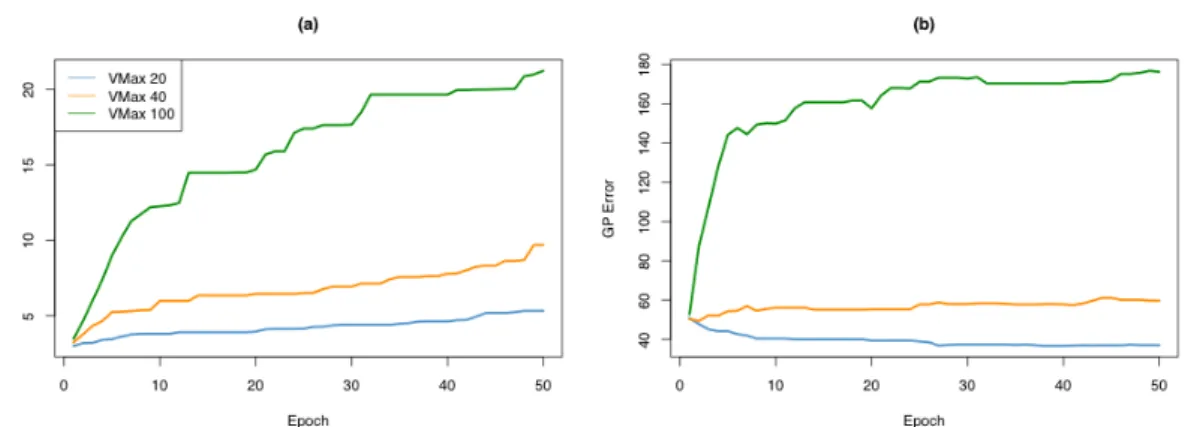
3.1 Results of running ODF V1 for the first time. Evolution of (a) delta error and the corresponding (b) GP error. The delta error denotes the difference between the GP error and GSGP error in favor of GP: the higher the delta error, the higher the dataset favorability is towards GP. The GP error is the RMSE value of the final solution produced by GP. Median values over 10 runs. . . 12

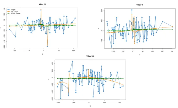
3.2 GBest position plotted against the predicted outputs of GP and the pre-dicted outputs of GSGP. Positions are given for VMax values of 20, 40 and 100. Each plot is the GBest position of the median run for the respective parameters. The y axis holds the independent variable and the x axis holds the dependent variable . . . 14

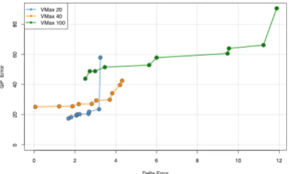
3.3 Local Pareto front of the median non dominant sets out of 10 MOPSO runs for VMax values of 20, 40 and 100. Each point in the plot represents a Pareto particle in the objective space. . . 15

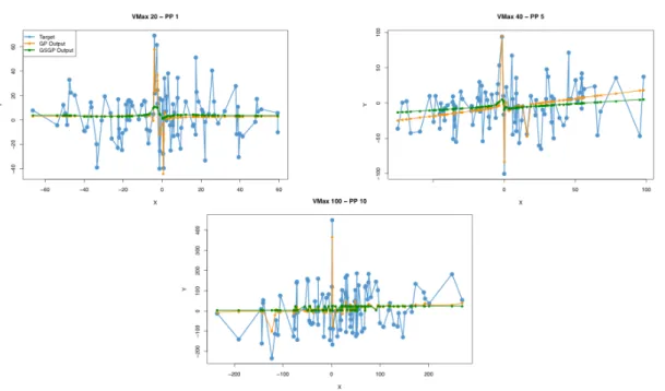
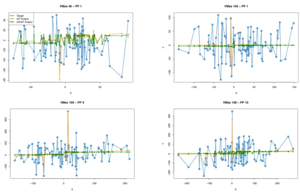
3.4 Positions of pareto particles from different non dominant sets, produced by different VMax settings. ‘PP’ in the titles stands for pareto particle. VMax 20 – PP 1 has a GP error of 19, VMax 40 – PP5 has a GP error of 28 and VMax 100 – PP 10 has a GP error of 90.. . . 16

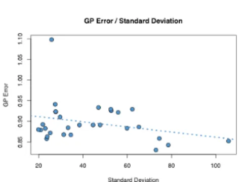
3.5 GP errors from all pareto particles from Figure 3 expressed against their standard deviation of the dependent variable and the regression line for this data. . . 17

3.6 Positions of pareto particles from different non dominant sets, produced by different VMax settings. ‘PP’ in the titles stands for pareto particle. VMax 40 – PP 1 has a delta error of 0, VMax 100 – PP1 has a delta error of 2.5, VMAX 100 – PP 9 has a delta error of 12 and VMax 100 – PP 10 has a delta error of 13. . . 17

3.7 GP NRMSE from all pareto particles from Figure 3 expressed against their standard deviation of the dependent variable. . . 19

(10)

L i s t o f F i g u r e s

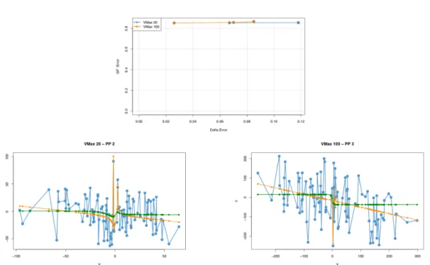
3.8 Positions of non-dominated particles in the objective space for the median runs with different VMax settings. The results were obtained with NRMSE turned on and outlier processing turned off. . . 20

3.9 Positions of two pareto particles produced by the ODF with VMAX 20 and VMax 100 respectively and the new NRMSE error function. . . 20

3.10 Local Pareto fronts (top plot) and the positions of selected particles (bot-tom plots) they contain. MOSPO was run with both NRMSE and outlier processing activated. . . 21

3.11 Perturbations of the non-dominated set. . . 21

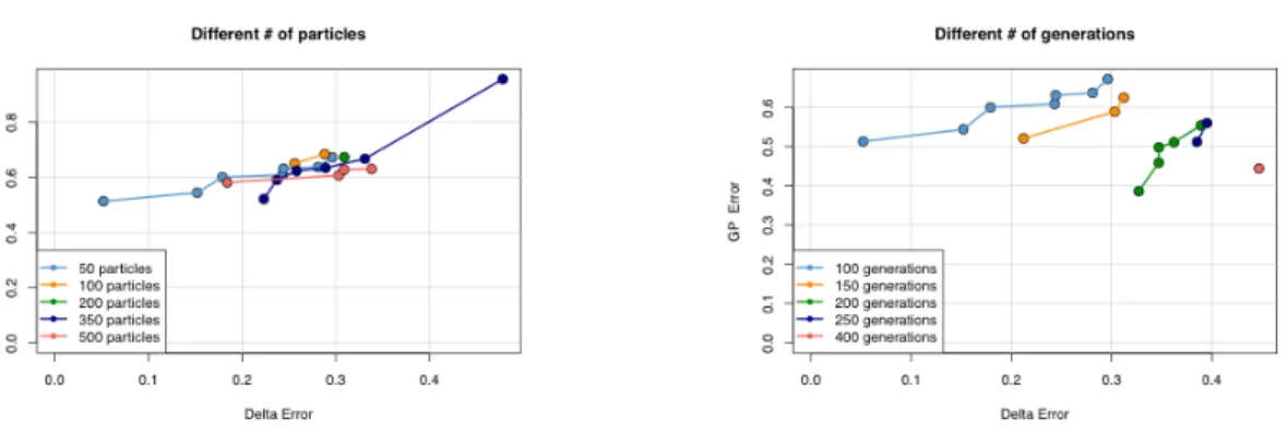
3.12 Comparison of local Pareto fronts produced by different particle settings and G(SG)P generation settings respectively. These results are obtained with the number of instances set to 30. . . 22

3.13 Comparison of local Pareto fronts produced by different particle settings and G(SG)P generation settings respectively. These results are obtained with the number of instances set to 30. . . 26

3.14 Validated results of the Evolution of GBest when optimizing delta errors in favor of GP and GSGP respectively. . . 27

3.15 Validated evolution of GSGP error of GBest for different number of variables. 28

3.16 Evolution of GBest when optimizing for GSGP on 20, 100 and 500 particles. 29

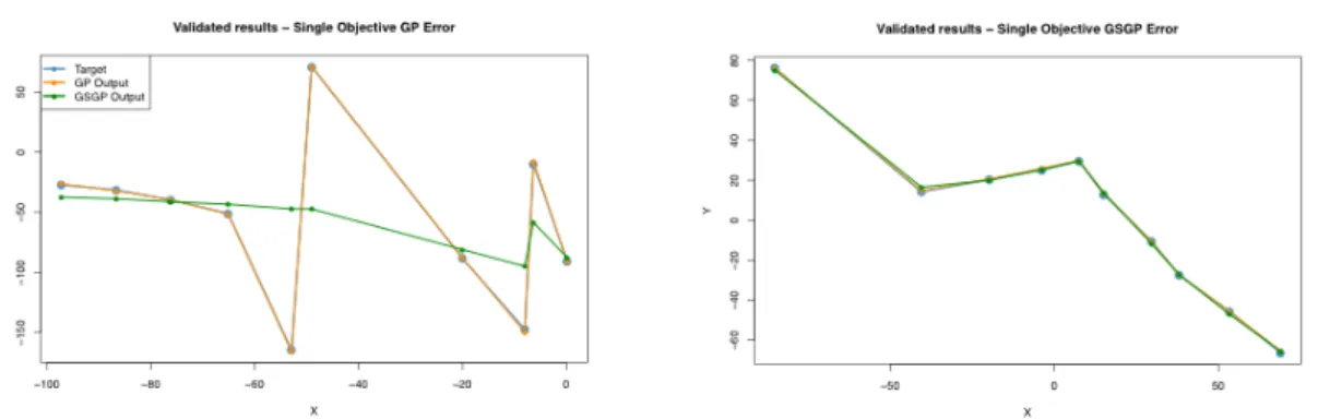
3.17 Original and validated evolutions of GP/GSGP errors for GBest solution when improving for GP as presented in Table 3.5.. . . 30

3.18 Original and validated positions of GBest after optimizing for GP as pre-sented in Table 3.5 with the corresponding GP and GSGP outputs. . . 31

3.19 Pareto fronts produced by the original ODF runs when optimizing for GP and GSGP separately on 2 and 3 dimensions. . . 36

3.20 Perturbations to the non-dominated sets per epoch when optimizing for GP and GSGP seperately using 2 and 3 variables. . . 38

3.21 Validated results for the Pareto fronts when optimizing for GP and GSGP separately using 2 and 3 variables. . . 38

(11)

List of Tables

3.1 Execution times of the ODF in hours for different settings of GP/GSGP and number of particles. . . 23

3.2 Original and validated results for optimizing datasets for GP and GSGP respectively. NRMSE was used as the objective function and the dataset consists of 10 instances.. . . 25

3.3 Original results for optimizing GSGP with delta error as the objective func-tion, using different number of variables.. . . 27

3.4 Original and validated NRMSE results for running the ODF with different number of particles while using NRMSE as objective function. The results are obtained from optimizing datasets for both GP and GSGP separately. 29

3.5 Original and validated results for optimizing datasets for GP and GSGP respectively. Delta error was used as the objective function and the dataset consists of 20 instances.. . . 30

3.6 Original results after running the ODF with different ranges for different optimizable algorithms and different objective functions: Optimizing for GP on NRMSE, optimizing for GP on delta error, optimizing for GSGP on NRMSE and optimizing for GSGP on delta error. . . 32

3.7 Validated results after running the ODF with different ranges for different optimizable algorithms and different objective function: Optimizing for GP on NRMSE, optimizing for GP on delta error, optimizing for GSGP on NRMSE and optimizing for GSGP on delta error. . . 32

(12)

Listings

2.1 Pseudocode for a basic PSO algorithm . . . 5

2.2 Pseudocode for a basic MOPSO algorithm . . . 8

(13)

Acronyms

GBest Global Best. A concept of Particle Swarm Optimization. The best solution found by all particles through all epochs (see Glossary).

GP Genetic Programming. A heuristic based optimization technique that uses tree structured genes to encode computer programs.

GSGP Geometric Semantic Semantic Genetic Programming. An altered implemen-tation of the Genetic Programming algorithm that uses geometric operators to search semantic space.

LBest Local Best. A concept of Particle Swarm Optimization. The personal best solution found by a particle (see Glossary).

MOOP Multi Objective Optimization Problem. An optimization problem that has more than one objective function that needs to be maximized/minimized. MOPSO Multi Objective Particle Swarm Optimization. A particle swarm

optimiza-tion algorithm that uses more than 1 objective funcoptimiza-tion.

NRMSE Normalized Root Mean Square Error. Root Mean Squared Error divided by the standard deviation of the dependent variable.

PSO Particle Swarm Optimization. A heuristic based optimization problem algorithm based on animal flock behavior.

RMSE Root Mean Square Error. A measure that indicates the accuracy of a model. VMax Velocity Maximum. A concept of Particle Swarm Optimization. The maximum

value for velocity (see Glossary).

VMin Velocity Minimum. A concept of Particle Swarm Optimization. The minimum value for velocity (see Glossary).

(14)

Terminology

Because of the use of multiple algorithms throughout this thesis there are a lot of different concepts and definitions that will be mentioned interchangeably through-out this paper. Some of these concepts could cause confusion because they are quite similar. For example, both Particle Swarm Optimization and Genetic Programming (algorithms used to optimize our problem, as discussed later) evolve their individual solutions by going through multiple iterations. If the word iteration would be used, it would not be clear for the reader whether the iteration of a GP/GSGP run or a PSO run is meant. It is important to have a clear distinction between concepts such as these so that there will be no confusion when reading this paper. It is also simply useful to have common terminology for often occurring definitions. For these purposes, below is a small list of definitions with their respective meanings.

Definitions for Genotype of the solutions

• Data Point: A point in n dimensional space, containing values of all dependent variables and the independent variable of one instance.

• Dependent variable: The variable that needs to be predicted by the symbolic regression engine, also known as the target variable.

• Independent variable: Variable that is used to build a model to predict the de-pendent variable.

• Instances: Observations in the dataset.

Definitions for Particle Swarm Optimization

• Cognitive Learning Factor: Factor that determines how much a particle is steered towards its own best found solution.

• Epoch: One iteration in the PSO algorithm.

• GBest: The best solution found by all particles through all epochs. The whole algorithm has only one GBest value.

• LBest: The best solution found by an individual particle through all executed epochs.

(15)

T E R M I N O L O G Y

• PBest: The personal best solution found by a particle. Every particle has their own PBest value.

• Position: The genotype of the solution, which is a dataset containing of m in-stances and n dimensions.

• Social Learning Factor: Factor that determines how much a particle is steered towards the global best found solution.

• Swarm: The entire population, which is made up of all the particles.

• Velocity: The direction and speed in which a particle “flies” through the search space.

• VMax/VMin: The maximum and minimum values for velocity.

Definitions for (Geometric Semantic) Genetic Programming • Error: The difference to the global optima, or the fitness of an individual • Generation: One iteration of the GP or GSGP algorithm.

• Individual: An individual member of the GP/GSGP population.

• Population: All solutions of the GP and GSGP algorithms, consisting of all the individuals

Definitions for Multi Objective Particle Swarm Optimization

• Local Pareto Front: The multi-objective equivalent of a local optimum: a Pareto front outputted by the algorithm that is not the true/global Pareto front.

• Pareto Front: The hyperplane in objective space on which the individuals lie with the best possible tradeoff between different objective functions.

• Pareto Particle: A particle of which it’s position is a member of the non-dominated set.

• Non-Dominated Set: A set of particles of which it’s position is not dominated by any other particle’s position found so far.

(16)

Introduction

1

In the field of symbolic regression, Genetic Programming (GP)[1] has been a popular algorithm to solve optimization problems. Geometric Semantic Genetic Programming (GSGP) [2] is an alteration of GP using geometric crossovers, which has been shown to outperform GP in real life applications [3] [4] [5]. As this introduction will further point out, numerous studies have been conducted to GP hardness but little to no research has been done towards GSGP hardness. Research towards GSGP hardness has so far been impossible due to the excellent performance of GSGP, leaving no to very little datasets which hare GSGP hard. The objective of this paper is to address this lack of GSGP hard datasets by designing and implementing an algorithm that generates datasets that are harder to solve for GSGP than for GP. This allows for effectively analyzing GSGP hardness for the first time.

Since the introduction of GP in 1992 [1] it has been widely studied and used in many fields, like climatology [6], cryptanalysis [7] and finance [8]. In 2011, M. Korns [9] researched accuracy in state-of-the-art symbolic regression. In said research, GP was used for the experiments and it was concluded that a serious issue exists for symbolic regression engines; even though a solution is returned with good fitness, this doesn’t mean that the correct formula is returned. In fact, even for very simple test problems consisting of one basis function with no noise and only a few features, GP is very often not able to return the correct formula to the user. It is stated that even simple test problems can have very large search spaces, hence the poor performance in accuracy.

To overcome this problem and to improve GP in general, different alternative implementations of the GP algorithm have been proposed throughout the years. One of those alternatives is Geometric Genetic Semantic Programming (GSGP) [2]. GSGP uses geometric operators that allow the algorithm to search in semantic space, thus being able to transform a solution’s genotype based on an alteration in its phenotype. The main advantage of this approach is that this creates a unimodal fitness landscape for any supervised learning problem, turning even complex fitness landscapes into simple fitness landscapes. The test results from Moraglio et al. [2] showed that this new implementation heavily outperformed GP.

(17)

C H A P T E R 1 . I N T R O D U C T I O N

The biggest limitation of GSGP on its introduction however, was the size of the solution. The geometric operators caused the solutions to grow exponentially, render-ing the program useless even within just a few generations because of the extensive computational power required to build and compute an individual. Vanneschi et al. [3] proposed a solution for this problem by using references (or memory pointers) instead of actually building every individual with every generation. This approach requires storing only the original population and the random trees (used by crossover and mutation) that are still used by any individual in the current generation. A third reference table is then used that holds the current solutions by “pointing” to the par-ent(s), the operator used and the random tree(s) used during the operation. This way, the individual is never actually build and only the semantics need to be computed.

This still left researchers with the problem that upon finishing the algorithm the solution is still too big to be constructed and thus to be used externally or logically interpreted (which has been recently addressed by J.F. Martins et al [10]), but it did allow for GSGP to be used on real life data. Upon using GSGP on real life data for the first time, it was shown that GSGP outperforms GP on training data and also, surprisingly at first, in terms of generalization ability [3] [4] [5]. After that, GSGP has successfully been applied to many different real life problems, like predicting concrete strength [11] [12], predicting the severity of Parkinson’s disease symptoms [13] and sentiment analysis [14].

GSGP’s performance on training data decreased by a little bit when a small alter-ation was made to the mutalter-ation [3] than originally proposed when GSGP was first introduced [2] by adding a logistic function to the random trees that are generated. This limits the output of the random trees in the interval [0,1]. Gonçalves et al. [15] researched the implications of this small alteration and found that the training error got higher with the new mutation implemented by Vanneschi et al. [3], but it per-formed significantly better in terms of generalization ability. The mutation was named bounded (BM) mutation [15] and became the standard for GSGP. Even though the training error of GSGP with BM on was higher than GSGP without BM, it still outper-formed GP on all but one dataset in said research and continues to outperform GP in other applications.

1.1 GP Hardness vs GSGP Hardness

It is known that there are a lot of problems where GP has difficulties converging to a desirable solution. Several researches have been performed towards GP hardness. M. Korns [9] researched several simple benchmark problems and found that some were hard for GP to solve. K.E. Kinnear [16] researched GP problem difficulty early after

GP’s inception by examining the structure of the fitness landscapes, which showed good correlation with problem difficulty. J.Daida et al. [17] investigated the role of structure on GP hardness. Their hypothesis was that structural mechanisms existed

(18)

C H A P T E R 1 . I N T R O D U C T I O N

[18] [19]. This implies that all possible tree structures can be divided into different categories based on a scale of hardness. The research states that most structures are difficult to create for GP, which might contribute to GP hardness.

M. Clerque et al. [20] researched if the fitness distance correlation (fdc), used earlier for measuring Genetic Algorithm difficulty [21], could also be used to measure GP problem difficulty and concluded that it is indeed a suitable problem difficulty metric. Vanneschi et al. [22] continued the research towards fdc as a GP difficulty

metric and confirmed that fdc is a suitable metric for this purpose but with some limitations, e.g. the existence of counterexamples (functions that are easy for GP to optimize while fdc says the opposite) and the global optima has to be known a priori. Therefore, they proposed another measure for GP problem difficulty that overcomes these limitations; negative slope coefficient (nsc). Vanneschi et al. [23] expanded on this research by pointing out that the nsc is not a reliable measure if a fitness cloud [24] is partitioned into arbitrary segments and proposed a more suitable way of partitioning the fitness cloud.

The research that has been conducted on GP problem difficulty is extensive and doesn’t limit itself to the researches mentioned above. While GP hardness has been researched quite well, there is no research to be found on GSGP hardness. In fact, the impression that the good performance of GSGP has raised seems to be that virtually any problem is easy to solve for GSGP. Not only is this contradictory to the No Free Lunch theorem [25], it is also unsubstantial to make such a statement without adequate research available towards GSGP problem difficulty. In this research we attempt to address the lack of research to GSGP hardness. Concretely, we propose an algorithm that generates datasets on which GP outperforms GSGP. Alternatively, the algorithm can be tuned to generate datasets in which GSGP performs better than GP, so that the results of both can be compared. A lot of different parameters come into play when designing such an algorithm. This paper presents the algorithm, its different parameters, the effect that different parameter values have on the outcome, and finally reports and discusses the findings that were derived from the results.

(19)

Background

2

This section explains the theory of the different algorithms and concepts that are used throughout this research: the Particle Swarm Optimization algorithm, the concepts of multi-objective optimization and Multi Objective Particle Swarm Optimization.

2.1 Particle Swarm Optimization

The original algorithm is a basic Particle Swarm Optimization (PSO) [26]. PSO is a heuristic based optimization technique which is based on animal flock behavior using swarm intelligence. One of the key features of PSO is that besides that solutions learn from their own search history, it is also social, i.e. the different solutions within the algorithm don’t just act independently from each other but they share information so that they can learn from each other. A couple of characteristics of the PSO algorithm made it a suitable choice for this research. Firstly, it is designed for continuous opti-mization problems, which is exactly the kind of problem we are dealing with in this paper. Secondly, considering the many different parameters already involved in this algorithm, PSO requires just a few parameters to adjust which reduces the complexity of an already complex algorithm. Thirdly, PSO is known to require low computational cost. This is a plus considering the heavy fitness function that is used for the algorithm (as will be presented later).

The entire population in PSO is called a swarm, which consists of particles. Each particle is an individual member of the swarm. GBest stands for global best and de-notes the best solution found by all particles over all executed iterations. An iteration in PSO is called an epoch. PBest stands for personal best and denotes the personal best found by a particle over all executed epochs, which means there are as many PBest values as there are particles. Velocity is the speed in which a particle “flies” through the search space. VMax and VMin are the maximum and minimum boundaries for the velocity value. The cognitive learning factor is a factor that determines how much a particle is steered towards its PBest value and the social learning factor is a factor that determines how much a particle is steered towards GBest. Every epoch the velocity is

(20)

C H A P T E R 2 . BAC KG R O U N D

calculated for every particle, which is then used to update the position of every parti-cle, where the position is the genotype of a particle. Equation2.1is used to update the velocity for a particle, after which2.2is used to update the position of a particle.

Vi(t + 1) = Vi(t) + c1ri1×(pbesti(t) − Xi(t)) + c2ri2×(gbest(t) − Xi(t)) (2.1) X_i(t + 1) = X_i(t) + V_i(t + 1) (2.2) Where i=1,2,3. . . ,n and n is the number of particles in a swarm. Xi(t) is the position

of the particle i at epoch t and V_i(t) is the velocity of particle i at epoch t. pbest_i(t) denotes the ith particle personal best found up and until the tth epoch and gbest(t)

denotes the global best found up and until the tth epoch. c1 is the cognitive learning

factor and c2 is the social learning factor. r1 and r2 are both random real value num-bers between the interval of [0, 1], which means they are a factor for the proportion in which a particle is steered towards the global best and how much it is steered towards their local best. The pseudocode of a basic PSO is given below:

Listing 2.1:Pseudocode for a basic PSO algorithm

1 Randomly initialize swarm

2 Evaluate each particle

3 While termination condition is not met

4 For every particle

5 Compute velocity according to Equation 1

6 If velocity > VMax

7 Velocity = VMax

8 If velocity < VMin

9 Velocity = VMin

10 Update position according to Equation 2

12 Evaluate Particle

13 If PBest is worse than current fitness

14 Current position is set to be new PBest

15 If GBest is worse than PBest

16 PBest is set to be new GBest

(21)

2.2 Multi Objective Optimization

Multi Objective Particle Swarm Optimization (MOPSO) is a PSO that is adapted to work with multi-objective optimization problems (MOOP) [27]. MOOP has 2 or more objectives that have to be optimized, where all different objectives are optimized simul-taneously. A solution to a multi-objective optimization problem is the best possible tradeoff between all given objectives. Formally, a MOOP can be represented as:

Minimize/Maximize fi(x), i = 1, 2, . . . , I

Subject to g_j(x) ≥ 0, h = 1, 2, . . . , J

hk(x) = 0, h = 1, 2, . . . , K xLm≤xi ≤ xLm, m = 1, 2, . . . , M

(2.3)

Where x is the decision vector and f_i is the ith objective function. g_j(x) and h_k(x) are inequality and equality constraints respectively. The last constraint, xL_m≤_x_i≤_xL

m,

constrains the variable xi to be within the lower bound xmL and the upper bound xLm.

A solution is said to be feasible if all constraints and variable limits are met. If it doesn’t, the solution is called infeasible. All feasible solutions together are called the feasible region. Comparing different solutions with a MOOP is more complex than with a single objective optimization problem since the results of more than 1 objective function have to be compared with each other. A way of comparing solutions in a MOOP is based on Pareto dominance [28] [29]. Assuming a maximization problem on all objective functions, the concept of dominance states that a solution x dominates a solution y (written as x ≺ y) when two conditions are met:

1. x is no worse than y for all objective values:

fi(xi) ≥ fi(xk); ∀k = 1, 2, 3, . . . , N

2. x is strictly better than y in at least one objective function:

f_i(x_i) > f_i(x_k); for at least one k ∈ 1, 2, 3, . . . , N

Pareto dominance uses the concept of dominance to rank solutions of a MOOP. Pareto dominance uses this ranking system to return a set of possible solutions. The ranking system is explained by a number of definitions [30] [31]:

Definition 1 (Non Dominated Set)

A vector of decision variables x ∈ S ⊂ Rnis said to be non-dominated if there exists no other x0∈_{S such that f (x}i_{) ≺ f (x).}

Definition 2 (Pareto Optimality)

A vector of decision variables x ∈ F ∈ R is said to be Pareto optimal if it is non-dominated with respect to the feasible region F.

(22)

Definition 3 (Pareto Optimal Set)

The Pareto optimal set contains all Pareto optimal solutions. Formally, the Pareto optimal set P∗is defined as P∗={x ∈ F|x is Pareto optimal}

Definition 4 (Pareto Front)

The Pareto front P F∗ are all the Pareto optimal solutions positions in the objective space. The Pareto front P F∗is formally defined as P F∗= {f (x) ∈ Rk|_{f (x) ∈ P}∗}

A MOOP based on pareto dominance thus tries to determine the pareto optimal set from the set F, which we call a globally Pareto front. Just like finding the global best in a single objective optimization problem is not a certainty, finding the global pareto optimal set is also not always achievable. A Pareto front that is produced by an algorithm that is not the true Pareto front is called a local Pareto front.

2.3 Multi Objective Particle Swarm Optimization

A number of changes have to be made to the original PSO algorithm so that it can op-timize multiple objective functions based on pareto dominance, which is called Multi Objective Particle Swarm Optimization (MOPSO) [32]. Firstly, the algorithm needs to store the non-dominated particles. Note that when we say non dominated particles, we refer to the non-dominated positions of the particles. These non-dominated particles are called leaders. Any of the leaders can be used to guide the search of a particle and every particle can choose a different leader at epoch t. This leads to a slightly altered velocity function as can be seen in equation2.4.

Vi(t + 1) = Vi(t) + c1ri1×(pbesti(t) − Xi(t)) + c2ri2×(Ph−Xi(t)) (2.4)

Where P is the external archive containing the non-dominated particles, Phis a

sin-gle leader that is selected from it and h is selected randomly from the non-dominated set. The external archive is updated with each epoch, at which all the currently non dominated solutions are entered into the archive and any solution in the archive that is now dominated is removed from the archive. Finally, PBest is chosen using Pareto dominance. If PBest and the new position both don’t dominate each other, one of them is randomly selected. The procedure of MOPSO is given in listing2.2.

(23)

Listing 2.2:Pseudocode for a basic MOPSO algorithm

1 Randomly initialize swarm

2 Evaluate each particle in the swarm

3 Setup non dominant set S

4 While termination condition is not met

6 Compute velocity according to equation 2.4

7 If velocity > VMax

8 Velocity = VMax

9 If velocity < VMin

10 Velocity = VMin

11 Update position according to equation 2.2

13 Evaluate Particle

14 If current position ≺ PBest

15 Current position is set to be new PBest

16 If both current position and PBest don ’t dominate each other

17 Randomly choose PBest

18 Update non - dominated set S

(24)

Methodology & Results

3

The main goal of the experiments that follow is to design and implement an algo-rithm which outputs a dataset consisting of dependent and independent variables, on which GP outperforms GSGP for symbolic regression problems. These solutions would then form a solid basis towards analyzing GSGP problem hardness, of which little to nothing is known to date. We want to emphasize that the focus is on designing and implementing an algorithm that is successfully able to produce solutions that meet the stated goal. However, analyzing these results so that definitive conclusions can be made as to what characteristics of a dataset define what makes an optimization problem GSGP hard is not the main goal of this thesis. It is however desirable and the aim is to draw conclusions wherever possible, but the main goal is to provide a foundation that can be used in future research towards GSGP hardness.

The original thought behind the thesis was simple: write an algorithm that produces data sets in which GP outperforms GSGP. It was at first also believed that the

implemen-tation of such an algorithm would prove to be not too complex either. As so often happens, reality proved differently and this thesis and the research behind it grew a whole lot bigger than initially expected. Actually, this research consists of multiple researches. Each research building upon the results of the previous researches: the first results led to observations, which led to the conclusion that the algorithm had to be altered in a way such that more desirable results would be achieved. The alterations led to new results, which led to new observations, which led to new changes in the algorithm and so on.

This section will therefore be divided into 5 sub-sections, where each sub-section represents a research phase. Each research phase is characterized by its own implemen-tation of the Optimal Dataset Finder (ODF) algorithm and/or its own research goals. Every research phase therefore has its own experimental setup and results. Since every subsequent research phase builds on the results of the previous research phase, the re-sults will be presented and discussed for every research phase separately. Even within a single research phase it is possible that the interpretation of experimental results led to new experiments within the same research phase. These sub-experiments still using the same algorithm and they are run with the same goals in mind that are applicable

(25)

C H A P T E R 3 . M E T H O D O L O G Y & R E S U LT S

to that research phase. This means that it is not uncommon for small new experiments to be proposed (and executed) in the results section of a given research phase.

Phase I proposes the initial ODF algorithm and runs the first experiments with it. Phase II proposes a new version of the ODF algorithm that is able to handle multiple objective functions. Phase III focuses on solving issues with the ODF that arose during Phase II and were deemed critical to solve. Phase IV goes in depth to different parame-ter settings and the effect they have on single objective functions. Phase V combines all knowledge from the previous research phases to try and evolve solutions that satisfy our goals. Lastly, the final ODF algorithm is shortly reviewed.

3.1 Phase I

Phase 1 presents the initial design of the ODF algorithm. The purpose of the algorithm is to output a data set in which GP outperforms GSGP. This means that the genotype of every particle is a matrix of size mn consisting of real numbers, where m is the number of instances and n is the number of dimensions. This is also the position of a particle and therefore represents the matrix X in equations 2.1, 2.2 and2.4. The variables in a symbolic regression problem consist of independent variables and dependent variables. In our case, we are always predicting 1 dependent variable. This means that there are n − 1 independent variables. The learning process for these datasets is a PSO run as described in section2.1at which in every epoch the velocity and positions are computed for each particle.

The fitness function is simple in terms of definition but complex in terms of com-putational effort. We are looking for datasets that are more suitable for GP than for GSGP. This translates itself into a maximization problem where the fitness metric is the difference between the fitness of GSGP and the fitness of GP. This means that both GP and GSGP have to be executed on the dataset in order to compute the fitness, which is expected to be computationally extensive but a necessity none the less. Formally, the fitness function f can be defined as follows:

f (X) = g(X) − h(X) (3.1)

Where g(X) is the fitness output of GSGP, h(X) is the fitness output of GP and f (X) needs to be maximized. Informally, the fitness output is the difference between the fitness of GSGP and the fitness of GP. GP and GSGP both use Root Mean Square Error (RMSE) as their fitness metric. It is formally defined in equation3.2

RMSE = v t _n X i=1 ( ˆy − y)2 n (3.2)

Where n is the number of instances, y is the predicted value of the dependent variable for the ith instance and ˆy is the actual value of the dependent variable for

(26)

the ith instance. The lower the RMSE, the better the individual. To avoid confusion

between the fitness of the PSO algorithm as outputted by equation3.1and the fitness of GP and GSGP as outputted by equation3.2, GP and GSGP fitness will from now on be referred to as simply GP Error and GSGP Error. The PSO fitness will be referred to as delta error. The PSO algorithm updates the velocity of a particle using equation2.1

after which the position of the particle is updated using2.2.

3.1.1 Experimental Setup

The number of variables is set to 2, so this means that we have 1 independent variable and 1 dependent variable. The reason we choose this number is for plotting purposes. Using only 2 variables makes it possible to plot the independent variable against the dependent variable on a 2D plane. This allows for visually analyzing and interpreting the outputted datasets such that we might be able to identify patterns and/or functions that determine what makes a dataset easier to solve for GP than for GSGP. The number of instances is set to 100 and the particles positions are initialized within the range [-100:100]. The swarm consists of 50 particles and the particles will evolve for 50 epochs. No other termination condition is set because we want the delta error to be as high as possible. Different values of VMax are used to see the effect it has on the delta error. Every variant of the PSO was run 10 times. The results presented in this paper are the median al of those 10 runs. Ideally, the number of runs would be higher but the heavy computational cost of the algorithm limits us in the number of runs (as will be pointed out later). For now this is deemed sufficient to get a good impression of the performance of the algorithm. Once the algorithm reaches a more final stage, solutions will be proposed to address the heuristic nature of the algorithm.

The algorithms used for the PSO fitness function are canonical GP and canonical GSGP. The function set consists of the four binary arithmetic operators +, -, * and / protected as used in early studies of GSGP [3] [4] [5] and as in [1]. The terminal set contains constants within the range [-1:1] with increments of 0.25, totaling to 9 constants in total. The total number of terminals will therefore be 9 + n, where n is the number of independent variables. The number of individuals is fixed to 50 and all GP and GSGP runs iterate over 100 generations. It might be argued that these values are low but they are set low intentionally. Keeping these settings low saves a lot of computational cost in an already computational expensive program. If these settings prove to be too low after analyzing the results, the settings will be altered accordingly.

The initialization method used is Ramped Half and Half [1] with maximum ini-tial depth set to 6 and selection is done with tournament size 2. GP uses standard crossover [1] and mutation [1], where crossover probability is set to 0.9 and mutation probability to 0.1. This means that crossover will be performed 90% of the time and individuals will be mutated 10% of the time. GP has a depth limit that is set to 17 to limit computational cost. GSGP uses a crossover rate of 0.0 and a mutation rate of

(27)

1.0, meaning that all the perturbations to individuals are done by mutation only as proposed in [15]. The only small alteration made to the canonical GSGP is that it uses bounded mutation (BM) [15]. Reason for this is because in real life applications GSGP would most likely use BM as well because of its good generalization ability. We are aware of the heuristic nature of both GP and GSGP but choose to run both algorithms only once none the less. Our first goal is to implement an algorithm that is able to produce suitable solutions. If we are able to reach this stage the heuristic nature of both GP and GSGP will be addressed accordingly. This approach saves much needed time in finding the right settings for the algorithm.

3.1.2 Results

The experimental results are presented through the curves of the delta error and the curve of the GP Error and describe the initial results of running the algorithm and the effect changing VMax has on the results. GP Errors are analyzed as well because it can lead to more insights about the behavior of the ODF. The plots mentioned above represent the median values for 10 PSO runs. We like the emphasize that we are aware that this is low for a heuristic based algorithm, but as we mentioned earlier this is a necessity because of the heavy fitness function. The heuristic nature will be further addressed at the more final stages of the algorithm. This is discussed more thoroughly in section 3.1.1. The median value is preferred over average values because of its robustness to outliers. The position of GBest after the last epoch is also plotted. These results are plotted against the predicted outputs of GP and GSGP.

Figure 3.1:Results of running ODF V1 for the first time. Evolution of (a) delta error and the corresponding (b) GP error. The delta error denotes the difference between the GP error and GSGP error in favor of GP: the higher the delta error, the higher the dataset favorability is towards GP. The GP error is the RMSE value of the final solution produced by GP. Median values over 10 runs.

Plots (a) and (b) of Figure 3.1show the evolution of the median delta error and the median GP error over all epochs. Three different values of VMax were used for this test: 20, 40 and 100. The results in plot (a) clearly show that the delta error rises

(28)

significantly when raising VMax. Even more so, the higher VMax, the longer and quicker the delta error rises. There seems to be no decline in the increase of delta error at 50 epochs when VMax is set to 100. These results would indicate that the algorithm is working well, as in it is doing what it is supposed to do: maximizing the delta error. Plot (b) shows that the GP error also grows significantly when raising VMax. In the early epochs the GP error skyrockets upwards when VMax is set to 100. After that the drastic increase in GP error makes room for a more steady, fluctuating increase during the remaining epochs. PSO with VMax set to 20 is the only run that decreases the GP error but upon finishing it has a delta error that is almost identical to the delta error at initialization.

Figure3.2shows the position of GBest for the median run for every different VMax

value. Each data point represents the independent variable (X axis) against the depen-dent variable (Y axis). The predicted outputs of GP and GSGP of GBest are plotted as well. All different VMax settings have an almost perfectly linear line running through approximately the center of the data points of GBest. What is also a common occur-rence is that all the positions have some extreme values which GP is able to predict pretty accurately, while GSGP is not able to predict them at all. In general the posi-tions still look very random but GP is able to adjust to the randomness a little more than GSGP. This explains why GP is “outperforming” GSGP as per the definitions of the algorithm. The range gets bigger for both GP and GSGP but their models stay the same, almost linearly running through the mean of the data points. However, since GP is able to predict some extreme values quite accurately, it is able to “outperform” GSGP in terms of delta error, but it comes with an increase of the GP error as well.

3.1.3 Discussion

it is safe to conclude that both the GP and GSGP models are equally bad for all differ-ent VMax values. In the field of symbolic regression we would not be interested in a model that takes the mean of data points (assuming the data points are spread out), nor are we interested in a model that does the same except for predicting 1 or 2% of the independent variable while totally missing the others. One can argue how suit-able a solution with high delta error is when the GP Error is very high as well. What good would a dataset that’s beneficial for GP be, if GP itself performs very poorly too? It could informally be stated that both GP and GSGP perform badly, but GP is the algorithm that performs a little less bad. If both algorithms perform very poorly, the results might be neglectable since any algorithm with this kind of performance wouldn’t stand in real life applications. Ideally we would want the difference to be as high as possible, while the GP error stays at low as possible. This indicates that we are not dealing with a single objective optimization problem but with a multi-objective optimization problem instead.

(29)

Figure 3.2:GBest position plotted against the predicted outputs of GP and the pre-dicted outputs of GSGP. Positions are given for VMax values of 20, 40 and 100. Each plot is the GBest position of the median run for the respective parameters. The y axis holds the independent variable and the x axis holds the dependent variable

3.2 Phase II

Phase II proposes a multi objective version of the original ODF algorithm. The goal of this phase is to successfully implement a multi objective variant of the ODF and to test different parameter settings to see which set of settings result in the best solutions.

The ODF was altered into a Multi-Objective Particle Swarm Optimization (MOPSO) as described in Section2.3consisting of 2 objective functions. The first objective function is the delta error as computed in Equation 3.1, which will have to be maximized. This function was also used in the first experiments as the only fitness function. The second objective function is h(x) from Equation3.1, which denotes the GP error that is computed as in3.2. The GP error is a minimization problem. In short, we are trying to maximize the delta error while simultaneously trying to minimize GP error. Since we do not know what kind of dataset patterns/functions we are looking for, there are no constraints that the solutions need to satisfy. All parameter settings were kept the same as in the previous experimental settings.

(30)

3.2.2 Results

Unlike the previous single objective PSO, MOPSO produces a set of possible solutions instead of just a single solution. This set of solutions will from now on be referred to as S. A single solution in S will from now on be named a pareto particle. Having multiple solutions returned leads to a different way of presenting and interpreting the results. MOPSO is run 10 times. The median run is not used because selecting the median run is not as straight forward when there’s multiple solutions with different objective functions, since this greatly limits the possibility of aggregating the results and comparing them. Instead, one run is selected manually by estimating which run produced a non-dominated set S that appears to hold pareto particles with average objective function values.

Figure 3.3:Local Pareto front of the median non dominant sets out of 10 MOPSO runs for VMax values of 20, 40 and 100. Each point in the plot represents a Pareto particle in the objective space.

Figure 3.3shows the local Pareto front for S, where the local Pareto front refers to the Pareto front that is produced by the ODF but does not necessarily resemble the true/global Pareto front. VMax set to 20 produced 9 pareto particles ranging approximately between a delta error of 1.6 and 3.2 and a GP error between 19 and 60. VMax set to 40 produced 10 particles ranging approximately between a delta error of 0 and 4.3 and a GP error between 25 and 43. VMax set to 100 produced 10 particles ranging approximately between a delta error of 2.5 and 12.5 and a GP error of 41 and 90. On first sight, VMax set to 40 seems to have produced the best set of solutions since the delta error is bigger than VMax 20 but it doesn’t increase the GP error as much as VMax 100 does. However, a GP error of 25+ still seems to be too high to represent even a slightly accurate model. A pattern can also be noticed in the different Pareto fronts of Figure3.3. The higher VMax is set, the higher the GP error seems to become. To further try to explain this phenomena, Figure3.4plots the position of one pareto particle for each VMax setting. The Pareto particles that are chosen to plot are the Pareto particle with the lowest GP error, the median GP error and the highest GP error over all different settings.

(31)

Figure 3.4:Positions of pareto particles from different non dominant sets, produced by different VMax settings. ‘PP’ in the titles stands for pareto particle. VMax 20 – PP 1 has a GP error of 19, VMax 40 – PP5 has a GP error of 28 and VMax 100 – PP 10 has a GP error of 90.

Figure 3.4 shows the position of the Pareto particles (denoted as PP in the plot titles) in increasing magnitude of GP error. VMax 20 - PP 1 has the lowest GP error, VMax 100 – PP 8 has the highest GP error and VMax 40 – PP 3 is in between. The GP and GSGP outputs for all Pareto particles are almost a linear line through the middle of the data points, just like with the previous experiments. VMax 40 and VMax 100 also show one or two extreme values that gets predicted accurately by GP but not at all by GSGP. The standard deviation of the data seems to get higher over the Pareto particles. VMAX 20 – PP 1 is clearly less spread out on the Y axis (independent variable) than VMax 40 – PP 3, which in turn is clearly less spread out than VMax 100 – PP 8. This indicates that there might be a correlation between GP error and the spread of the data.

Figure3.5shows data for all Pareto particles of the different median non-dominated sets that were produced during this experimental phase. Every point in the plot repre-sents a Pareto particle’s standard deviation of the dependent variable (y axis) against the Pareto particle’s GP Error (y axis). The dotted line is the regression line for this data. It is evident that GP error and standard deviation are very highly correlated. The Pearson’s R value is 0.995, indicating a nearly perfect positive correlation between GP Error and the standard deviation of the dependent variable.

The increase in delta error is analyzed in a similar way as the increase in GP error was. Two of the lowest delta errors were picked from all non-dominated sets and com-pared to the two Pareto particles with the highest delta errors from all non-dominated

(32)

Figure 3.5: GP errors from all pareto particles from Figure 3 ex-pressed against their standard deviation of the dependent variable and the regression line for this data.

sets. The positions of these Pareto particles are plotted in Figure 3.6 against their respective GP and GSGP outputs. VMax 40 – PP 1 and VMax 100 – PP1 have low delta errors, while VMax 100 – PP 9 and VMax 100 – PP 10 have high delta errors. A difference between the positions of pareto particles with high and low delta errors is an outlier that is present. VMax 100 – PP 9 and VMax 100 – PP 10 both have an extreme outlier that GP is able to predict quite accurately, while GSGP is not able to predict it at all.

Figure 3.6:Positions of pareto particles from different non dominant sets, produced by different VMax settings. ‘PP’ in the titles stands for pareto particle. VMax 40 – PP 1 has a delta error of 0, VMax 100 – PP1 has a delta error of 2.5, VMAX 100 – PP 9 has a delta error of 12 and VMax 100 – PP 10 has a delta error of 13.

(33)

3.2.3 Discussion

In order to get the GP error down, the algorithm is shrinking the spread of the data instead of finding a data set that better fits a model produced by GP. Thus, the algo-rithm is doing what it’s programmed to do (minimizing GP error) but not doing it in a way that was expected, nor in a way that satisfies our objectives. A smaller GP error at this stage simply means a smaller spread of the data as proven in Figure3.5, not a better fitted model. Besides that, the ODF also seems to be increasing the delta error by producing an outlier. This outlier is accurately predicted by GP but not by GSGP, hence the increase in delta error. The further the outlier is removed from the rest of the data, the further the increase in delta error. After seeing these results MOPSO was run more times and this behavior of increasing the delta error was confirmed. It is very likely that this result is simply because of an overfitted model and therefore not behavior that we want to see in the ODF. Even if it wasn’t due to overfitting, a model that predicts only one value accurately can’t be considered a good model.

To summarize, the algorithm is successfully able to both lower the GP error and to increase the delta error, but not doing so in the way that is desired. The “shortcuts” that are being taken by the ODF probably prevents the algorithm from actually searching for datasets in which it is able to better fit a model. Instead, the ODF is searching for data that better fits a linear model through the center of the data. Firstly, an adjustment has to be made to the algorithm so that the spread of the data is not correlated anymore with the GP error. This will force the ODF to look for other ways of reducing the GP error, hopefully by producing data sets where GP is able to fit a better model. Secondly, the algorithm needs to be prevented from producing outliers to boost the performance of GP compared to GSGP, which is not able to predict these outliers but GP is. The same goes here: if this behavior is restricted, hopefully the ODF will find more suitable ways of improving the datasets.

3.3 Phase III

Phase 3 focuses on addressing the main issues that were discovered in the previous research phase. The goal of this phase is to resolve these issues. Alterations to the ODF are proposed to prevent the ODF from shrinking the spread in order to lower the GP error and to prevent the ODF from producing outliers. Once these issues are resolved, experiments are run to see if the updated ODF is able to evolve the datasets in a way such that the datasets actually become more favorable for GP.

(34)

Figure 3.7: GP NRMSE from all pareto particles from Figure 3 ex-pressed against their standard de-viation of the dependent variable. To address the problem of the ODF shrinking the

standard deviation of the data in order to shrink the GP error, an alteration to the fitness function is implemented. The RMSE from Equation 3.2

is divided by the standard deviation of the inde-pendent variable, which we will call Normalized Root Mean Squared Error (NRMSE). From now on, when we refer to GP error, GSGP error or delta error we are always referring to the NRMSE value. The terms GP/GSGP Error and NRMSE will be used interchangeably. A NRMSE of 0 means the model predicts all independent vari-ables perfectly, a NRMSE of 1 means the model is simply a linear line through the center of the data

points as seen in our experiments, thus solving the problem of the algorithm seeing a linear line through the center as a good solution. 3.7 plots the same Pareto parti-cles from Figure3.3, but this time using the new NRMSE value instead of the RMSE value. It proofs that the correlation between the GP error and standard deviation of the earlier tested data is now non-existent after applying the normalization step. An additional big benefit is that all errors are now range independent. This allows for comparing solutions with different data, e.g. a dataset that has its data points within the range of [0:1] with a NRMSE of 0.5 performs equally as good as a dataset in the range [-1,000:1,000] with a NRMSE of 0.5.

An additional alteration is made to the algorithm to address the “shortcut” of outlier generation in order to improve GP error, as discussed in Phase II. Before a particle is evaluated, their positions go through an outlier removal phase. The outliers that need to be removed are the outliers in the independent variable. An outlier is considered an outlier if it is below Q1 − (1.5 × IQR) or above Q3 + (1.5 × IQR), where

Q1 is the first quartile of the particles set of independent variables, Q3 is the third

quartile of the same set and IQR is the interquartile range. If an outlier is found it is replaced by a random value that lies between the current Q1 and Q3. The ODF is run with the same settings as before but now only limiting the runs to VMax values of 20 and 100. PSO is first run with only the new NRMSE fitness measure turned on to see the effects of this by itself. After this, outlier processing is turned on as well to analyze the changes in outcome this new feature has by itself.

3.3.2 Results

The results are obtained in the same way as with the previous experiment/ MOPSO is run 10 times for each setting and the run that appears to have average results is hand

(35)

selected.

Figure 3.8: Positions of non-dominated particles in the objective space for the median runs with different VMax settings. The results were obtained with NRMSE turned on and outlier processing turned off.

To first see the effects of the new NRMSE fitness measures, Figure3.8 presents the local Pareto fronts without the proposed outlier processing mechanism turned on. Where the earlier used RMSE function produced around 10 Pareto particles per non dominated set S, the new NRMSE function produces not more than two Pareto particles in a non-dominated set. This number was higher for some other runs but still a lot less than before. This implies that the algorithm has a harder time finding solutions now it is restricted from taking “shortcuts” in finding better solutions. The fact that the solutions are not able to go below a GP error of 0.8 strengthens this assumption. Next to the GP errors being similar for different VMax settings there also seems to be no significant difference in delta error.

The GP error values of 0.8 translate into the positions of the pareto particles as seen in Figure3.9. Both models show an almost linear line through the center of the data, which is what is expected with a high GP error of 0.8, thus the new measure is successful in penalizing the way it was previously improving the GP error. The

Figure 3.9:Positions of two pareto particles produced by the ODF with VMAX 20 and VMax 100 respectively and the new NRMSE error function.

(36)

Figure 3.10:Local Pareto fronts (top plot) and the positions of selected particles (bot-tom plots) they contain. MOSPO was run with both NRMSE and outlier processing activated.

Pareto fronts in Figure3.10show the local Pareto fronts produced by the ODF with now also outlier processing turned on. The delta errors of these Pareto particles are noticeably lower compared to the Pareto fronts produced without outlier processing. This indicates that the ODF now has a harder time increasing the delta error since it is limited in producing outliers that are only predictable by GP. The positions of the two Pareto particles with the highest delta error confirm this assumption. VMax 20 – PP2 still has a somewhat big value but it is not nearly as extreme as the outliers produced with outlier processing turned off.

Figure 3.11: Perturbations of the non-dominated set.

The ODF is now not showing unwanted be-havior anymore as in that it is taking “shortcuts” to falsely indicate that a solution is getting bet-ter. The solutions are, however, far from desirable since they do not represent accurate models in the slightest. It is highly probably that the solution to this problem is not to be found in a different VMax value or increasing the number of epochs as can be concluded after looking at Figure3.11. The plot shows the size of S at every epoch and the amount of additions and deletions performed in that epoch. There are not a lot of perturbations

(37)

Figure 3.12:Comparison of local Pareto fronts produced by different particle settings and G(SG)P generation settings respectively. These results are obtained with the num-ber of instances set to 30.

taking place throughout the entire ODF run and even if the Pareto front would con-tinue evolving like this indefinitely, which is highly improbable, it would take months to produce an acceptable solution. Two other parameters, which have intentionally been kept low so far to save computational cost, that might improve the performance of the ODF are the number of particles and the number of generations for GP and GSGP.

To research the effect of changing the number of particles and generations, the number of instances has been lowered to 30. The reason for this being the very big increase in computational effort with the increase in both parameters (Table 1). VMax has been fixed to 50. Changing the number of particles doesn’t result in any real improvement to the produced solutions as can be seen in Figure3.12. There is a slight difference but nothing that leads to believe that increasing the number of particles has a positive effect on the ability the ODF has on finding a suitable solution.

Changing the number of generations clearly does lead to an overall improvement in the solutions found by the ODF. The local Pareto front moves beneficially with every increase of the number of generations. However, it doesn’t seem like improving the generations would lead to the ODF producing desirable solutions since it doesn’t seem like the GP error will converge somewhere close to 0 anytime soon. Even if it did, it would not be able to do so within reasonable limits: raising the number of generations increases the execution time of the ODF significantly, as can be seen in Table3.1.

(38)

C H A P T E R 3 . M E T H O D O L O G Y & R E S U LT S Generations 100 200 300 400 Particles 50 0.74 2.36 4.2 6.17 150 2.06 6.38 14.62 18.78 300 3.42 12.96 30.25 37.33 Table 3.1:Execution times of the ODF in hours for different settings of GP/GSGP and number of particles.

3.3.3 Discussion

The implementation of the new NRMSE measure effectively solved the problem of the ODF reducing the standard deviation of the dataset in order to reduce the error of both GP and GSGP. However, the ODF doesn’t come anywhere near converging to a satisfiable solution. This indicates that in this state, it’s not possible for the ODF to find other ways of improving the solutions, i.e. by finding data sets that GP is actually better able to fit its models on. The same goes for the new outlier processing step. It does solve the problem it’s designed to address, but it makes it even harder for the ODF to evolve the solutions. It also doesn’t seem like changing VMax can have that much of an impact to get the ODF to produce suitable solutions. Instead, we assume that the solution lies in the number of GP/GSGP generations and the number of particles.

Both parameters have intentionally be kept low so far to limit computational cost. Also, it was argued that it might produce even better solutions when these parameters are kept low. The reasoning behind this was that if the ODF is able to find solutions at only 100 generations that have very low GP errors and very high delta errors, it would surely imply that a dataset is very easily solvable by GP but very difficult for GSGP. Since this assumption has not been able to be proven so far, different particle and generation settings were used. Increasing the number of particles did not noticeably improve the solutions, but improving the number of generations did. That the increase in the number of generations would lead to a decrease in GP error was expected since GP/GSGP has more time to fit its model. However, it also leads to a noticeable increase in delta error, implying that the it does more than just allowing GP/GSGP to evolve for longer. That the increase in particles did not lead to better results was not expected considering that the search phase is infinite for every instance. With a search space that big, one would expect that more particles would surely lead to better performance.

Either way, the ODF is not coming anywhere near converging to a solution that allows for analyzing GSGP hardness effectively. It also doesn’t seem that any of the tried parameters will influence the performance of the ODF enough to achieving such solutions. The optimization problem proves to be too complex at this complexity level, so it is believed to be beneficial to take a step back by starting from a low complexity level and build up the complexity from there. This can be done by lowering the number

(39)

of instances even further, evolving the ODF successfully on that number of instances, and then raise the number of instances to do the same on the new complexity level. Using single objective optimization instead of multi objective optimization lowers the complexity level as well, plus that it might lead to valuable insights. Knowing what minimizes the GP/GSGP error and what maximizes the delta error separately would be valuable knowledge that allows for targeted parameter setting.

3.4 Phase IV

Previous experiments with MOOP have not yet been able to produce solutions that can be used to effectively analyze GSGP hardness: both the GP error and the delta error are not nearing convincing values. Therefore it is decided to focus on one of the measures first instead. Specifically we would like the GP error to be as low as possible, but so far it has not been anywhere near to closing in on zero, nor did it look like it would anytime soon. If we would know what settings lead to a low GP error, that knowledge could be integrated in MOPSO which would in turn produce better results as well. The same can be said about knowing what settings lead to a high delta error, independently from the GP/GSGP error.

Focusing on these objectives separately allows for a more scoped research to the optimization problem at hand. Thus, this phase does not focus on multi-objective optimization, but once again on single objective optimization. Unlike in the first phase however, we are not only maximizing the delta error but also minimizing the GP or GSGP error, depending on the goals of the experiment. The goal of this phase is to gain insights towards the effect of different parameter settings on GP/GSGP error, which in turn can then be applied to the multi objective version of the ODF. This is done by starting from a low complexity problem (low instances & single objective) and building up in complexity from there.

The algorithm is altered so that it only produces datasets that minimizes the GP error or maximizes the delta error, reverting it back to a single objective PSO. Firstly the focus will be on producing datasets that minimize the GP error. After this research has been concluded, attempts will be made to produce datasets that minimize the GSGP error. The starting point of this research will be a dataset with only 10 instances. If good results are obtained for this number of instances, the number of instances will be increased. This allows us to build our way up to increasing levels of complexity while reducing computational complexity. GP/GSGP generations are raised to 700 generations. This decreases the chance of a too low number of generations being the reason why the ODF is not able to converge to a solution. The number of epochs are set to 15. All other settings remain the same as with the previous experimental phase.