A Multi-Population Hybrid Genetic Programming System

(1)

A Multi-Population Hybrid Genetic Programming

System

Bernardo Gil Câmara Galvão

Dissertation presented as partial requirement for obtaining

šZ

D

_{•š Œ}

_[

_•

_PŒ

_]v

_{Advanced Analytics}

(2)

NOVA Information Management School

Instituto Superior de Estat´ıstica e Gest ão de Informaç ão

Universidade Nova de Lisboa

A MULTI-POPULATION HYBRID GENETIC PROGRAMMING

SYSTEM

by

Bernardo Galv ˜ao

Dissertation presented as partial requirement for obtaining the Master’s degree in Infor-mation Management, with a specialization in Advanced Analytics

Advisor: Dr. Leonardo Vanneschi

(3)

ABSTRACT

In the last few years, geometric semantic genetic programming has incremented its popularity, obtaining interesting results on several real life applications. Never-theless, the large size of the solutions generated by geometric semantic genetic programming is still an issue, in particular for those applications in which read-ing and interpretread-ing the final solution is desirable. In this thesis, a new parallel and distributed genetic programming system is introduced with the objective of mitigating this drawback. The proposed system (called MPHGP, which stands for Multi-Population Hybrid Genetic Programming) is composed by two types of sub-populations, one of which runs geometric semantic genetic programming, while the other runs a standard multi-objective genetic programming algorithm that op-timizes, at the same time, fitness and size of solutions. The two subpopulations evolve independently and in parallel, exchanging individuals at prefixed synchro-nization instants. The presented experimental results, obtained on five real-life symbolic regression applications, suggest that MPHGP is able to find solutions that are comparable, or even better, than the ones found by geometric semantic genetic programming, both on training and on unseen testing data. At the same time, MPHGP is also able to find solutions that are significantly smaller than the ones found by geometric semantic genetic programming.

KEYWORDS

(4)

LIST OF FIGURES

A.1. Effect of cosine function - Bioavailability (%F) . . . IX

A.2. Effect of cosine function - PPB . . . X

A.3. Effect of cosine function - Toxicity (LD50) . . . XI

A.4. Effect of cosine function - Concrete . . . XII

A.5. Effect of cosine function - Energy . . . XIII

A.6. Effects of varying migration rate - Bioavailability (F%) . . . XVI

A.7. Effects of varying migration rate - PPB . . . XVII

A.8. Effects of varying migration rate - Toxicity (LD50) . . . XVIII

A.9. Effects of varying migration rate - Concrete . . . XIX

A.10. Effects of varying migration rate - Energy . . . XX

A.11. 2-subpopulation MPHGP vs. MOGP and GSGP - Bioavailability

(%F) . . . XXXII A.12. 2-subpopulation MPHGP vs. MOGP and GSGP - PPB . . . XXXIII A.13. 2-subpopulation MPHGP vs. MOGP and GSGP - Toxicity (LD50)XXXIV

A.14. 2-subpopulation MPHGP vs. MOGP and GSGP - Concrete . . XXXV

A.15. 2-subpopulation MPHGP vs. MOGP and GSGP - Energy . . . . XXXVI A.16. Introspection of 2-subpopulation MPHGP - Bioavailability (%F) . XXXVIII A.17. Introspection of 2-subpopulation MPHGP - PPB . . . XXXIX

A.18. Introspection of 2-subpopulation MPHGP - Toxicity (LD50) . . . XL

A.19. Introspection of 2subpopulation MPHGP and MPHGP*

-Concrete . . . XLI

A.20. Introspection of 2-subpopulation MPHGP - Energy . . . XLII

A.21. Introspection of 2-subpopulation MPHGP* - Energy . . . XLIII

A.22. Performance of higher number of subpopulations - Bioavailability

(%F) . . . XLV

A.23. Performance of higher number of subpopulations - PPB . . . . XLVI

A.24. Performance of higher number of subpopulations - Toxicity

(LD50) . . . XLVII A.25. Performance of higher number of subpopulations - Concrete . . XLVIII

(6)

(7)

LIST OF TABLES

2.1. Description of test problems . . . 6

2.2. Synthesis of the parameter tuning for the tested MPHGP-2

system . . . 7

2.3. Changes in subpopulation size, tournament size, number of elite

survivors and number of migrants according to the increasing

number of subpopulations. . . 13

A.1. Statistical significance of cosine function, according to Wilcoxon

Rank-Sum tests - Bioavailability (%F) . . . XIV

Rank-Sum tests - PPB . . . XIV

Rank-Sum tests - Toxicity (LD50) . . . XIV

Rank-Sum tests - Concrete . . . XIV

Rank-Sum tests - Energy . . . XIV

A.6. Wilcoxon RankSum test on training error and unseen error

-Bioavailability (%F) . . . XXI

A.7. Wilcoxon Rank-Sum test on size and depth - Bioavailability (%F) XXI

A.8. Continuation of Table A.6. . . XXII

A.9. Continuation of Table A.7. . . XXII

A.10. Wilcoxon RankSum test on training error and unseen error

-PPB . . . XXIII

A.11. Wilcoxon Rank-Sum test on size and depth - PPB . . . XXIII

A.12. Continuation of Table A.10. . . XXIV A.13. Continuation of Table A.11. . . XXIV A.14. Wilcoxon RankSum test on training error and unseen error

-Toxicity (LD50) . . . XXV

(8)

A.16. Continuation of Table A.14. . . XXVI A.17. Continuation of Table A.15. . . XXVI A.18. Wilcoxon RankSum test on training error and unseen error

-Concrete . . . XXVII A.19. Wilcoxon Rank-Sum test on size and depth - Concrete . . . XXVII A.20. Continuation of Table A.18. . . XXVIII A.21. Continuation of Table A.19. . . XXVIII A.22. Wilcoxon RankSum test on training error and unseen error

-Energy . . . XXIX A.23. Wilcoxon Rank-Sum test on size and depth - Energy . . . XXIX

A.24. Continuation of Table A.22. . . XXX

A.25. Continuation of Table A.23. . . XXX

A.26. Rank-Sum test results, for MPHGP-2 - Bioavailability (%F) . . . XXXVII A.27. Rank-Sum test results, for MPHGP-2 - PPB . . . XXXVII A.28. Rank-Sum test results, for MPHGP-2 - Toxicity (LD50) . . . XXXVII

A.29. Concrete - Rank-Sum test results in terms ofp-values, for

MPHGP*-2 . . . XXXVII

A.30. Rank-Sum test results, for MPHGP*-2 - Energy (f = 25,

r= 0.35) . . . XXXVII A.31. Wilcoxon Rank-Sum tests on training and unseen errors for an

increasing number of subpopulations - Bioavailability (%F) . . . L

A.32. Wilcoxon Rank-Sum tests on unseen and training errors for an

increasing number of subpopulations - PPB . . . L

increasing number of subpopulations - Toxicity (LD50) . . . L

increasing number of subpopulations - Concrete . . . L

increasing number of subpopulations - Energy . . . LI

A.36. Median running time with increasing number of subpopulations LIV

A.37. Statistical significance of impact of number of subpopulations on

running times and size - Bioavailability (%F) . . . LIV

running times and size - PPB . . . LIV

running times and size - Toxicity (LD50) . . . LV

(9)

(10)

1 INTRODUCTION

Genetic Programming (GP) [Koz92] is a machine learning algorithm (typically used for supervised problems) that aims at finding programs - mathematical func-tions or computer programs - that best map inputs to outputs. It is called “genetic” due to the inspiration it takes from evolutionary biology. GP in fact belongs to the Evolutionary Computation class of algorithms.

A GP algorithm evolves a population of individuals (i.e. the programs) over the course of a prefixed number of generations. The evolution within a generation is carried out by the selection phase and the variation phase. The selection phase selects individuals (i.e. programs) based on their fitness into the variation phase - where fitness is captured by a set of objective functions to be optimized.

The variation phase is a means to search for fitter individuals by manipulating the ”genome” of the individuals - i.e. the genotypic (or syntactic) content of the program. In standard GP this is typically a crossover with a randomly selected crossover point or a mutation with a randomly selected mutation point. For a tree-based representation of programs, both these operations replace subtrees of a parent which consequently results in a new offspring. It should be noted that there are several other possible crossover and mutation operators. Each of these programs is considered to be an individual and a population of individuals is evolved for a prefixed number of generations. At the end of the evolution, the algorithm returns the fittest individual.

In recent years, many efforts to improve GP were undertaken [VCS14]. In par-ticular, Moraglio et al. [MKJ12] found variation operators that have known effects on the semantics of the offspring individuals [Van17] - where semantics are de-fined by the vector of outputs of a program on the different training data. These operators constitute Geometric Semantic Genetic Programming (GSGP). The ge-ometric semantic (GS) crossover and GS mutation operators are correspondingly defined as:

(11)

and

TM U =ms.(TR1−TR2) +T

Wheremsis the mutation step constant; R,R₁ andR₂ are random real functions

with codomain [0,1]; and T, T₁ and T₂ represent parents of the offspring. The

semantics of a crossover offspring are the result of a geometric mean of the semantics of its parents, hence, regarding distance to the global optimum, the offspring cannot be worse than the worst of its parents.

GS mutation corresponds to a ball mutation that induces a unimodal fitness land-scape [Van17] in supervised learning problems. A unimodal fitness landland-scape is that which is constituted by a single local optimum: the global optimum. To convince oneself of this property, any individual that is not the global optimum in the semantic space has at least one neighbor whose semantics are closer to the target values. To put it simply, there is virtually no risk of the algorithm being stuck in the non-existent local optima. It must be noted, this is one of the reasons this work opted to undertake only GS mutation, therefore excluding GS crossover. However, GSGP comes at a cost regarding size of found solutions: GS operators take the entirety of the nodes of the parents to produce the offspring. This results in a linear size growth if using GS mutation and exponential growth if using GS crossover. In order to circumvent this issue, an efficient implementation of GSGP proposed by Castelli et al. [Cas+13] (which is used in this thesis) allowed for the application of GSGP in real-world datasets [Van+13]. It essentially puts aside building the genotypic constitution of individuals, thus evolving the population us-ing only the semantics which are obtainable by the definition of the GS operators. Despite this, offline reconstruction (i.e. after evolution) still remains a problem due to the large size of GSGP individuals. Even when possible, readability and interpretability of the model produced by GSGP remains an issue.

In contrast, GP is not aggressive in size growth, at least by construction of its variation operators. Nevertheless, GP can incur in bloat, which is defined as the growth in size of the program without an improvement in fitness. In spite of GP facing the bloat issue, its solutions are yet acknowledged as parsimonious enough for readability and interpretability, being considered one of its main advantages [Koz10]. It is worth mentioning that such property of GP solutions ”shines” when bloat-limiting methods are used [SC09] [Tru+16] or when fitness and size are conjointly optimized in a multi-objective framework [VSD09].

Regarding performance of GSGP versus GP, it is important to note that GP is

(12)

operations on the syntax of individuals. This makes it frequently unable to find solutions that are competitive with those found by GSGP in terms of training error. In terms of unseen error, there is indication for the potentially better generalization ability [Van17] of GSGP on three pharmacokinetic datasets [Van+13] that are presented in this work as well.

(13)

2 MULTI-POPULATION HYBRID GENETIC

PROGRAM-MING

The proposed MPHGP system presented here has two types of subpopulations, one running multi-objective genetic programming (MOGP) and another one run-ning GSGP. The former optimizes size and trairun-ning error and the latter optimizes only training error. Each subpopulation is assigned to a thread and evolution is carried out by running each in parallel. MPHGP is completely implemented in Java, which carries out and handles parallelism with the class Thread. The synchronization instants correspond to moments of migration between the

sub-populations. These are prefixed by the migration frequency parameter f, i.e.

migration moments occur every f generations, thus each subpopulation evolves

independently duringf generations.

Following Fern ´andez et al. [FTV03], the migration direction is configured as a ring for any number of subpopulations. This means that if there are two subpop-ulations, the ring configuration corresponds to a simple exchange of individuals between the two subpopulations. If the number of subpopulations is, for instance, three, then subpopulation 1 sends its best individuals to subpopulation 2; sub-population 2 to 3; and finally, subsub-population 3 sends migrants to subsub-population 1.

In order to provide a comparative framework, this work considers standalone ver-sions denoted by MOGP and GSGP. The hybrid system is denoted by MPHGP (Multi-Population Hybrid Genetic Programming) and to refer its subpopulations, the terms sub-MOGP and sub-GSGP are employed. MOGP, GSGP and MPHGP run with a population size of 400 individuals each. Thus, if MPHGP has two sub-populations, this means that sub-MOGP and sub-GSGP run with 200 individuals each. All these variants are initialized using Ramped-Half-Half-Initialization [Koz92].

The migration policy isbest-to-worst, meaning that the individuals selected to

(14)

size of the overall population of MPHGP constant, a copy of these best individu-als remains in the origin subpopulation, so as to not waste the genetic material found by the evolution of that subpopulation. Except where noted, the selection of best individuals to migrate changes according to the optimization criteria of the subpopulation: in sub-GSGP, this means simply picking the fittest; in sub-MOGP, to follow a multi-objective policy, this means picking the fittest starting from the

best pareto front. Other migration policies, such asrandom-to-randomor

best-to-randomare not explored in this thesis.

In a view to address cross-domain robustness of the approaches, these three GP variants are tested in 5 real-world symbolic regression problems described by Table 2.1. The problems %F, PPB and LD50 [Arc+07] pertain to problems in pharmacokinetics research aiding drug discovery - respectively to human-oral bioavailability, plasma protein binding level and toxicity. These problems use as in-put a set of molecular descriptors of a potential new drug. The Concrete [CVS13] problem pertains to predicting the strength of this material according to its fea-tures and the Energy [Cas+15] problem refers to predicting the energy consump-tion using as input meteorological data of that and previous days, for instance. All of these problems have already been used in previous GP studies. These problem sets cover different degrees of dimensionality as proxies to their level of difficulty. Finally, to address optimization and generalization ability, these datasets are split into 70% for training data and 30% for unseen (test) data and the median Root Mean Square Error (RMSE) of 30 independent runs is reported.

It ought to be noted that the %F dataset faces criticism due to the presence of raw data and missing data that ideally would be cleaned up and transformed beforehand. This cannot be the case for this thesis. From the perspective of developing a machine learning technique, it is preferable to observe its behavior with a hard dataset. Moreover, GP is a machine learning technique that performs data transformations and feature selection with its evolutionary process. Such behavior ought to be nurtured namely, its ability to work around hard data -when designing new approaches to GP.

2.1 I

NTRA

-

POPULATION

C

ONFIGURATION

(15)

Dataset # Features # Instances

Bioavailability (%F) [Arc+07] 241 206

Protein Plasma Binding Level (PPB) [Arc+07] 626 131

Toxicity (LD50) [Arc+07] 626 234

Concrete [CVS13] 8 1029

Energy [Cas+15] 8 768

Table 2.1.:Description of the test problems. For each dataset, the number of features (independent variables) and the number of instances (observations) are re-ported.

individuals whose depth is well beyond a traditional depth limit of 17. For exam-ple, a depth limit mechanism works by rejecting an offspring if its depth is beyond the limit (and keeping one of the parents as replacement) and only accepting oth-erwise. Enabling depth limits would mean making MOGP be a storing sub-population that would just return sub-GSGP individuals from previous migration instants. Furthermore, MOGP that includes size as an objective to be minimized is aggressive in reducing size of individuals: notice how an individual with only one node is in the first pareto front regardless of its uselessness in capturing the complexities of the dataset and its training error. The selection mechanism -pareto rank selection (NSGA-II) - is thus going to consider such small individuals as among the fittest.

GSGP uses the aforementioned efficient implementation [CSV15] and has a crossover rate of 0. This is justified because geometric semantic mutation does not increase size as dramatically as geometric semantic crossover would, making MPHGP testable in useful time - notice that GSGP individuals have to be built at each migration instant and that MOGP cannot work on these individuals offline! Note that GS mutation builds up from a single individual rather than from two entire in-dividuals. This is also convenient in offline rebuilding of the fittest individual after an evolution has ended, and, in the context of MPHGP, at migration instants: with

only mutation, each individual has only a single parent, and after g generations,

the fittest individual will haveg ascendants to look up in the offline records. 1 _In

the opposite extreme case of only crossover, each individual will have two

par-ents, meaning that the winning champion will have to be rebuilt upon 2g _parents

and looking up such an amount of individuals is an expensive task itself. For this reason, crossovers are handled by sub-MOGP only, which will be in charge of making crossovers between sub-GSGP individuals and its own small

individu-1_{I.e. the hash tables storing the references to relevant individuals in the history of the evolution}

(16)

Parameter MOGP GSGP

Objectives training error and size training error

Crossover Rate 0.9 0

Elitist Survival 5 5

Tournament Size 15 15

Parent Selection Method Pareto Rank Selection Tournament Selection

Mutation Step - 1.0

Bounded Mutation - Yes

Migrant Selection multi-objective single-objective

Table 2.2.:Synthesis of the parameter tuning for the tested 2-Population Hybrid Genetic Programming (MPHGP-2) system. In order to provide a comparative basis, standalone MOGP (with 400 individuals) and standalone GSGP (with 400 individuals as well) follow the same tuning as the one reported here for the MPHGP-2 subpopulations, each of which with a size of 200 individuals. Multi-objective migrant selection means picking the fittest from the first pareto rank, then from the second pareto rank and so on.

als.

The cosine function is included along with protected division, multiplication, addi-tion and subtracaddi-tion operators. Generally it improves fitness, generalizaaddi-tion ability and reduces size. Please refer to Figures A.1 to A.5 and Tables A.1 to A.5, where standalone MOGP and GSGP are measured against their equivalents without the cosine operator. It is observed that regardless of the dataset, the cosine operator allowed for a reduction in size for GSGP while improving or retaining training error and (or) unseen error - except for the exquisite LD50 dataset. Differences are not notable in MOGP due to the aforementioned issue that it cherishes a small num-ber of nodes excessively, which may have hindered this algorithm from actually taking advantage from the cosine function the way GSGP did. For this reason, the cosine was opted to be included in the MOGP subpopulations of MPHGP, a context in which sub-MOGPs will definitely be operating with individuals of greater sizes that they receive from sub-GSGPs.

(17)

The number of elite survivors is unusually high and fixed at 5. Considering the case of MOGP, which has a tendency of being blind to optimization quality in favor of lower size, this is meant to keep the fittest individuals in place of the smallest of the new generation with no comparable quality - hence, the selection of elites and deletion of the worst individuals was purely single-objective even in MOGP. In the case of GSGP, this is based on the idea of growth along generations: individuals from previous generations are expected to be smaller than those of the current generation [CVP15]. Elitism in GSGP is used not only under the perspective of keeping solutions of better fitness but also of keeping other solutions that may slow down size growth.

Similarly to the number of elite survivors, the tournament size is high as well. It follows the rule of 7.5% of subpopulation size with a minimum constraint of 3 indi-viduals - this pertains to a higher number of subpopulations, which is mentioned in Section 2.4. For a 2-population MPHGP, this equates to 15 individuals. Re-garding MOGP (remind that it uses ”pareto rank selection” from NSGA-II), in the event that very small solutions are randomly drawn to the selection phase, it is de-sirable that such solutions do not have an excessively higher probability of being selected than solutions of better optimization quality, and increasing tournament size is equivalent to approximating to a uniform density function. In the case of GSGP, this increases the chances of finding the fittest solution, given tournament selection.

2.2 I

NTER

-P

OPULATION

P

ARAMETER

T

UNING

For the analysis of a 2-population MPHGP system, the effect of varying two mi-grational parameters is discussed in this section. The first one is the migration

frequencyf, which is defined as the number of generations that each

subpopu-lation uses to evolve independently from the other one. The second parameter to

be discussed is the migration rater, the percentage of the subpopulation size that

determines the integer number of migrants. For instance, if the MPHGP system is split into two subpopulations, each will have a size of 200 individuals. Then, for a migration rate of 0.15, MOGP will send its best 0.15 * 200 = 30 individu-als to GSGP and this subpopulation in its turn will return its fittest 30 individuindividu-als

to MOGP. This study covers migration frequencies{25, 50, 100} that result

cor-respondingly to {12, 6, 3} migration instants in 300 generations; and migration

rates{0.05, 0.15, 0.25, 0.35}that correspond to{15, 30, 45, 60} individuals

(18)

parameters that were ran for the 5 datasets across 30-independent runs.2

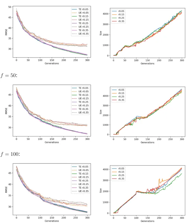
For each dataset, Figures A.6 to A.10 show on the left-hand side line plots for the median training and unseen errors, where unseen errors are portrayed by dotted lines; and a right-hand side plot for the size. Each row in each these figures

pertains to a migration frequency f and all migration rates are plotted together.

One observes that migration rates are generally ineffective in median terms, at least for a given migration frequency.

To further look into this matter, matrices of p-values for the Wilcoxon Rank-Sum

test - testing whether two samples come from the same distribution - between the results of two migrational parameter combinations are provided in Tables A.6 to A.25. If one wants to check for the statistical significance of effects of migration rate for a given migration frequency, one only needs to look at the “blocks” in the diagonal of these tables. In most cases, there is close to no difference in varying the migration rate for a fixed migration frequency. The ”blocks” standing outside

the diagonal represent cross-frequencyp-values. In these cases, the difference is

more noticeable, indicating the higher impact of varying migration frequencies.

Overall the combination f = 50 and r = 0.15 seemed to obtain the best results

across the datasets. For this reason and the sake of simplicity, the migrational parameters are generally fixed to these values and the analysis in the following

sections is to be seen as one ofcoeteris paribus.

2.3 2-P

OPULATION

H

YBRID

G

ENETIC

P

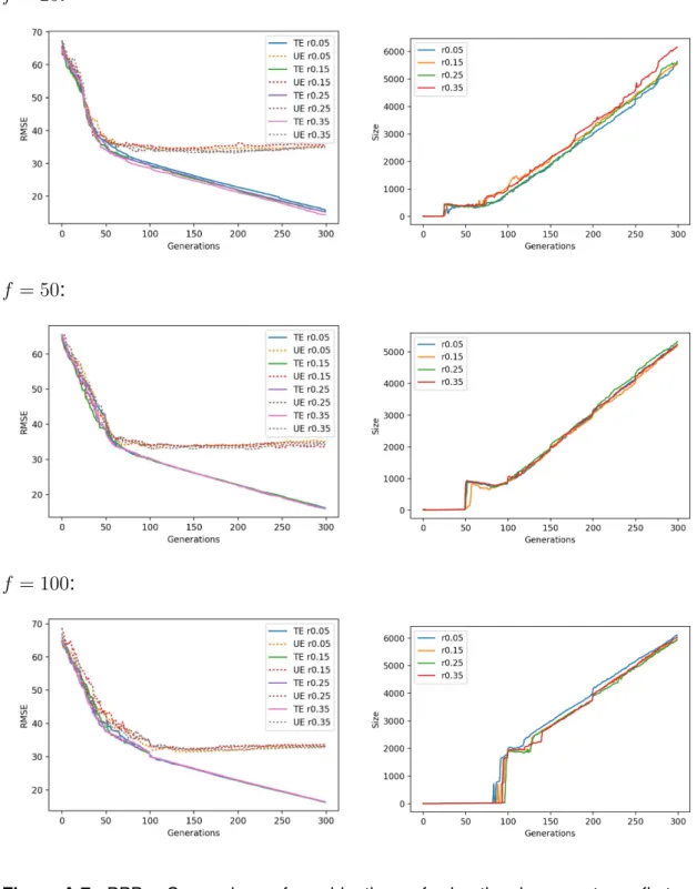
ROGRAMMING

The work included in this section is already published and was presented by the author in an international conference [VG17]. The results presented pertain to migration frequency 50 and migration rate 0.15 for a MPHGP with two subpopu-lations, except where noted. In this section it is attempted the study of MPHGP against the standalone MOGP and GSGP versions as well as the exercise of studying the relationship between GSGP and MOGP subpopulations of MPHGP - these are denoted as sub-MOGP and sub-GSGP in the introspection Figures A.16 to A.21.

The reported results show that MPHGP is able to at least retain the best training and unseen errors from the subpopulations. In some cases, improvement on one

2_{Please note that this resulted in}₁₂_∗₃₀_∗_{5 = 1800}_{runs just for MPHGP results pertaining to this}

(19)

of these measures can be observed. General statements cannot be made about the obtained size of solutions for a 2-population hybrid system.

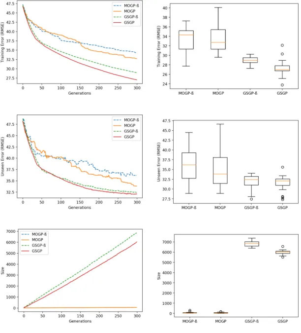
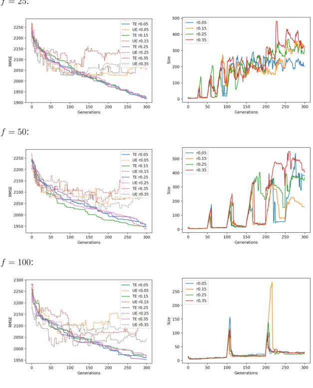
In the Bioavailability case (Fig. A.11 and Table A.26) MPHGP retained the training error and improved both unseen error and size. To understand how the algorithm got to this outcome, it is useful to look into the behaviour of each subpopulation in Fig. A.16. Note that MPHGP picks the best individual on training error from the two subpopulations to be reported, and each subpopulation reports only its best individual on training error to be reported as well. The first migration event takes place after evolving generation 50, at which point sub-GSGP is leading on training error, thus these fitter individuals emigrate to sub-MOGP, which causes not only sub-MOGP to improve its fitness but also to take in the size of these individuals, causing the spike in its median size at generation 50.

It is after this moment that sub-MOGP takes over the lead of MPHGP, suggesting that its NSGA-II selection mechanism and standard variation operators are more suitable for the sub-GSGP individuals at this moment of the evolution of MPHGP. Leadership in training error is important to help determine what way size will shift to at each migration event. With this notion in mind, one can observe that size of sub-GSGP shifted downwards at migration instants of generation 100 and 150: it is because sub-GSGP applied its operators on the fitter and smaller individuals that came from sub-MOGP and updated its best individual accordingly. For the remaining generations, sub-GSGP takes back the leadership and does not stem away from its size evolution trajectory anymore as sub-MOGP becomes a passive participant of MPHGP.

This aspect is important to the success of a basic hybrid system: each subpopu-lation ought to be an active participant in the evolution process and this is verified with the exchange of leadership in fitness between the subpopulations. To put it in other terms, what use would be of MPHGP if sub-GSGP led throughout the entire evolution? Is MOGP contributing at all in this case? Would it not be bet-ter to run only GSGP instead with offline reconstruction of individuals and end the run sooner instead of forcing MOGP to build large individuals? One has to ensure active participation of all subpopulations in MPHGP to reach the goals of this algorithm.

(20)

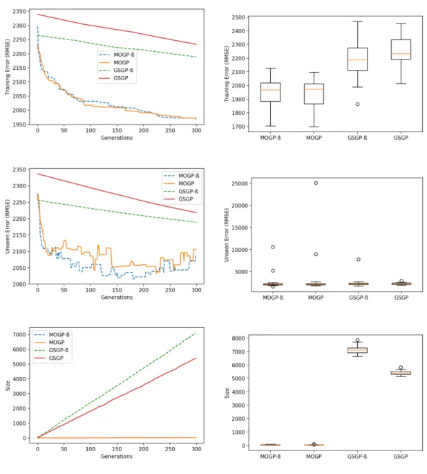
sub-MOGP has the lead before the first migration instant, and concedes it indefinitely to sub-GSGP from this moment onwards. The main observation one can make is that there is only one size reduction event that takes place in the evolution of MPHGP: at the first migration instant (generation 50) when sub-MOGP dominates in training error and in size. As no fitter and smaller individuals from sub-MOGP arise in the remaining generations of the evolution of MPHGP, sub-GSGP runs on its own and sub-MOGP merely becomes a follower. MPHGP finds a more par-simonious solution (in terms of size) than GSGP due to this single occurrence. Refer to Table A.27 for the statistical significance of these results.

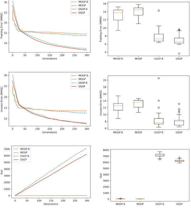
In the Toxicity dataset, MPHGP was only better in terms of training error - Fig. A.13 and Table A.28. In fact the best performing algorithm for 300 generations was MOGP with the lowest reported median unseen error and size. When looking into introspection (Fig. A.18), it is verified that GSGP played the passive role throughout all of the 300 generations. It is also observable that the spikes in size occurred only with the migration moments every 50 generations, meaning that the fittest on training error from MPHGP lied in the sub-MOGP. Further proof that MPHGP gravitated towards solutions of MOGP lies in Table A.28, where one can observe that MPHGP does not differ significantly from MOGP.

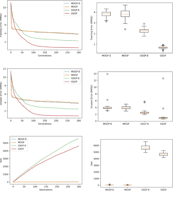
Finally for the Concrete and Energy datasets, statistically significant size reduc-tion was not achieved by employing the base MPHGP. A special strategy - de-noted by MPHGP* - to be able to achieve this result with two subpopulations can be synthesized by force-feeding sub-MOGP individuals into sub-GSGP. For this goal, two changes were applied to MPHGP:

• The selection of emigrants in sub-MOGP is single objective on training error,

so as to increase the chances of these individuals of being selected in sub-GSGP.

• Sub-GSGP only sends one individual to sub-MOGP.

(21)

This suggests that in the case of MPHGP*, sub-MOGP* individuals were being more frequently mutated and performant in sub-GSGP*, even becoming the fittest in some runs. If this is the case, then there is support for MPHGP: there is no full reliability on the first migration instant nor on the hope that MOGP leads at such moment. This means that another way to improve MPHGP could be to properly tune or find better algorithms for each of the subpopulations.

For the Energy dataset (Fig. A.15 and Table A.30), MPHGP* had its migration frequency dropped to 25 (Figures A.20 and A.21, respectively) in order to take advantage of the leadership of sub-MOGP* at this moment of the evolution, caus-ing sub-GSGP* to “reset” the size of its fittest individual after the first migration instant. In fact, the difference in size between MPHGP* and MPHGP and GSGP is due to this single “reset” and one can observe that despite this gap, the growth trend of MPHGP is identical to that of GSGP. Yet significant size decrease was achieved as showed in Table A.30.

This closes the study of a 2-population MPHGP system. In general, this system with basic configurations was able to keep the performance in training and unseen error of the standalone versions, or even improve in some cases. With regards to size, this strategy is not robust, which justified running MPHGP* with its tweaks. Nonetheless, active participation (leadership exchange on training error) of all subpopulations is important for the effectiveness of a basic MPHGP algorithm on reducing size of found solutions when two different subpopulations are evolving individuals in different size ranges. In other words, it is necessary to ensure that subpopulations run on par with each other in terms of training error in order to achieve the important “collaboration” between them. The case of the Concrete dataset showed that, in spite of having MOGP be a passive participant, sub-MOGP can still influence sub-GSGP to bring down the size of solutions.

2.4 I

NCREASING

N

UMBER OF

S

UBPOPULATIONS

(22)

Number of Subpopulation Tournament Elite

Migrants

Subpopulations Size Size Survivors

2 200 15 5 30

4 100 7 5 15

8 50 3 5 7

20 20 3 5 3

40 10 3 5 1

Table 2.3.:Changes in subpopulation size, tournament size, number of elite survivors and number of migrants according to the increasing number of subpopula-tions. Overall population remains constant at 400 individuals. Tournament size obeys to the rule of 7.5% of subpopulation size with a floor constraint of 3. Number of migrants obeys to the constant migration rater = 0_.15_{. It is} attempted to study the impact of only changing the number of subpopulations.

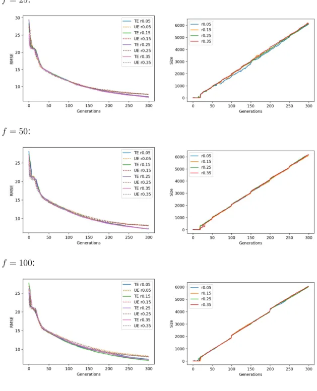
The number of subpopulations tested were 4, 8, 20 and 40. In order to capture the effect of varying only this parameter as much as possible, only tournament size was adapted for each number of subpopulations and is determined by a rule of [0.075 * subpopulation size] subject to a minimum of three. In order to have a clear picture of how these runs were performed, please refer to Table 2.3. Increasing the number of subpopulations generally proved to be effective in reducing the size of the solutions found.

For the Bioavailability dataset (Fig. A.22, Table A.31), and for an increasing num-ber of subpopulations, median training error increased slightly, but generalization ability of the solutions found by MPHGP was kept and their respective sizes de-creased. This can be considered a successful experiment that is also verified for the PPB (Fig. A.23, Table A.32) and Energy datasets (Fig. A.26, Table A.35). The effect of decreasing size seems to reach a plateau at 8 subpopulations for the Bioavailability and PPB datasets. Since increasing the distribution of the popu-lation yet retains the generalization ability, one may state that 40 subpopupopu-lations is optimal for the cases of Bioavailability, PPB and Energy, as computation time decreases as discussed in section 2.5.

(23)

(24)

2.5 R

UNNING

T

IMES

The results in this section correspond to the following available data on running times:

• MOGP-ß, standalone multi-objective GP, optimizing training error and size,

without the cosine operator.

• GSGP-ß, standalone single objective Geometric Semantic Genetic

Pro-gramming, without the cosine operator.

• MPHGP*-2, the MPHGP with two subpopulations, where MOGP selects

mi-grants on training error only and GSGP only sends one individual to MOGP.

Withf = 5 andr = 0.5.

• The remaining MPHGPs are those of Section 2.4, with the number of

sub-populations increasing.

• For the Energy dataset, the migration frequency is set to 25; for the

remain-ing datasets it is set to 50.

As mentioned before, increasing the number of subpopulations reduces the size of the best found solution, which contributes to having less nodes being evalu-ated per average individual in the population. Furthermore, subpopulations run in parallel until the prefixed migration instant, which means that more computation is being performed simultaneously, in the sense that instead of having one thread going over each of 400 individuals sequentially, there are, for instance, 20 threads going sequentially over just 20 individuals at the same time.

These two factors both contribute to the decreasing computation time with in-creasing number of subpopulations as verified in Fig. A.27 and in Fig. A.36. The only exception would be for the Toxicity dataset - which always yielded better results with MOGP for 300 generations - where the size of the best found in-dividual increased with the number of subpopulations, by tending to sub-GSGP solutions.

(25)

3 CONCLUSION

This thesis proposed a hybrid model to combine a multi-objective GP and GSGP, two subpopulations that run independently until a prefixed migration instant or synchronization moment when the two subpopulations exchange individuals. The experimental results on five real-world symbolic regression problems show that MPHGP is able to retain the advantageous properties of any of the algorithms while finding statistically significant smaller solutions, namely, than GSGP.

There are caveats to this work however. Firstly, while MPHGP was able to de-crease size, such solutions remain yet greater than desirable for the interpretabil-ity and readabilinterpretabil-ity in any of the problems. Thus, this work ought to be seen as one of first step in that direction.

Moreover, the increase in size of MPHGP solutions as generations go by fol-low the same trend as GSGP for a 2-Population Hybrid system, except for the Bioavailability (%F) dataset. Increasing the number of subpopulations helped getting away from such trend, mainly because of the compacter search-space of each subpopulation, which ”allowed” for the subpopulations to be on par with each other more frequently, thus exchange of individuals was more valuable. Secondly, the bar was lowered with using only mutation in GSGP: size growth is linear, as well as the number of ascendants of an individual. This allowed for the reconstruction of individuals to be trivial at each migration instant. This decision was undertaken for the sake of executing runs in useful time in a setting where MOGP would be responsible for crossovers. Hence, the crossover was never semantically aware and that is a case to be covered when the challenge of dealing with exponential growth is well handled.

(26)

errors of GSGP, in some cases it boosted one of these measures!3 _{Such a fact}

would have gone unnoticed without this extra work and it shows that sub-GSGP and sub-MOGP can complement each other.

Future work includes new research paths. Notice that there are several GP vari-ants out there that can be included in a hybrid system and it is yet to be known how well they would interact in such environment or how well they would benefit or benefit from GSGP. In specific, some of the most sophisticated known algo-rithms of simplification of mathematical expressions [ZZS05] ought to be included among the subpopulations of MPHGP. Given the results presented by this work, it is a given that these simplification algorithms will not be carrying out such a task by themselves!

An ambitious future work is to define a dynamic and versatile parallel and dis-tributed hybrid GP system. While this work was rather parsimonious in the param-eter configuration, ideally one can build a hybrid system that subjects to evolution number and size of subpopulations; algorithms executed in different subpopula-tions; and respective parameters. As a result, these would change during the run according to specific criteria.

3_{Fig. A.13 for an example of a boost on training error; Fig. A.11 for an example of a boost on}

(27)

A APPENDIX: FIGURES AND TABLES OF RESULTS

(28)

(29)

(30)

(31)

(32)

(33)

%F Train Unseen Size

MOGP-ß vs MOGP 0.74987 0.22102 0.50378

GSGP-ß vs GSGP 2.84E-05 0.13591 1.92E-06

Table A.1.:Bioavailability (%F) - Statistical significance of cosine function according to p-values Wilcoxon Rank-Sum tests. Significance at 5% is highlighted in light grey, stating that the distribution of results differs.

PPB Train Unseen Size

MOGP-ß vs MOGP 0.00057 0.44052 0.13779

GSGP-ß vs GSGP 0.06871 0.17138 1.73E-06

Table A.2.:PPB - Statistical significance of cosine function according to p-values Wilcoxon Rank-Sum tests. Significance at 5% is highlighted in light grey, stating that the distribution of results differs.

LD50 Train Unseen Size

MOGP-ß vs MOGP 0.97539 0.81302 0.11080

GSGP-ß vs GSGP 0.00148 0.29894 1.73E-06

Table A.3.:Toxicity (LD50) - Statistical significance of cosine function according to p-values Wilcoxon Rank-Sum tests. Significance at 5% is highlighted in light grey, stating that the distribution of results differs.

Concrete Train Unseen Size

MOGP-ß vs MOGP 0.01852 0.02564 0.06408

GSGP-ß vs GSGP 0.01752 0.65833 1.73E-06

Table A.4.:Concrete - Statistical significance of cosine function according to p-values Wilcoxon Rank-Sum tests. Significance at 5% is highlighted in light grey, stating that the distribution of results differs.

Energy Train Unseen Size

MOGP-ß vs MOGP 0.95899 0.71889 0.03222

GSGP-ß vs GSGP 1.73E-06 0.00003 1.73E-06

(34)

(35)

f = 25:

f = 50:

f = 100:

(36)

f = 25:

f = 50:

f = 100:

(37)

f = 25:

f = 50:

f = 100:

(38)

f = 25:

f = 50:

f = 100:

(39)

f = 25:

f = 50:

f = 100:

(40)

f 25 50

r 0.05 0.15 0.25 0.35 0.05 0.15 0.25 0.35

0.05 - 0.41653 0.00129 0.02703 0.01108 0.00499 0.02304 0.01397 0.15 0.47795 - 0.22888 0.18462 0.11561 0.13591 0.10639 0.12044 0.25 0.58571 0.97539 - 0.68836 0.47795 0.81302 0.92626 0.61431 25

0.35 0.32857 0.08972 0.21336 - 0.53044 0.39333 0.64352 0.34935 0.05 0.57165 0.08972 0.23694 0.99179 - 0.62884 0.33886 0.89364 0.15 0.55774 0.09777 0.19152 0.92626 0.64352 - 0.55774 0.97539 0.25 0.78126 0.08590 0.06268 0.84508 0.86121 0.74987 - 0.95899 50

0.35 0.99179 0.24519 0.29894 0.79710 0.81302 0.73433 0.65833 -0.05 0.02564 0.00468 0.00773 0.04950 0.04070 0.06871 0.05193 0.11093 0.15 0.14139 0.00567 0.01044 0.21336 0.04950 0.11561 0.10201 0.08590 0.25 0.00039 0.00241 0.00316 0.01397 0.01657 0.02183 0.00984 0.01397 100

0.35 0.28021 0.12544 0.17138 0.44052 0.58571 0.45281 0.59994 0.41653

Table A.6.:Bioavailability (%F) - Wilcoxon Rank-Sum test on training error and unseen error. Null hypothesis assumes that two samples (of results) come from the same distribution. Below the marked diagonal lie the p-values for tests on training error and above for unseen error. At 5% significance level, the cases which reject the null hypothesis is highlighted in light grey. The purpose is to visualize the impact of varying migrational parameters.

f 25 50

r 0.05 0.15 0.25 0.35 0.05 0.15 0.25 0.35

0.05 - 0.42242 0.76552 0.06711 0.72656 0.84506 0.90992 0.62881 0.15 0.85313 - 0.69589 0.37088 0.38705 0.28477 0.49722 0.30850 0.25 0.84508 0.45281 - 0.13320 0.88821 0.89362 0.99179 0.97538 25

0.35 0.45901 0.51705 0.21715 - 0.22877 0.12795 0.07268 0.20974 0.05 0.38203 0.24519 0.86121 0.09570 - 0.98359 1.00000 0.93442 0.15 0.74987 0.39333 0.84508 0.11800 0.86121 - 0.91808 0.97538 0.25 0.90993 0.47795 0.92626 0.14704 0.55774 0.81302 - 0.96718 50

0.35 0.44052 0.25364 0.84508 0.15886 0.84508 0.78126 0.51705 -0.05 0.89364 0.74986 0.26230 0.99179 0.44052 0.41653 0.81302 0.54401 0.15 0.82901 0.87740 0.50957 0.81302 0.34935 0.61431 0.81302 0.68836 0.25 0.01522 0.02849 0.00585 0.01657 0.00241 0.00567 0.02703 0.00064 100

0.35 0.84508 0.61431 0.88551 0.23694 0.92626 0.70356 0.74987 0.90993

(41)

f 100

r 0.05 0.15 0.25 0.35

0.05 0.03872 0.00129 0.12044 0.00411

0.15 0.03501 0.06564 0.53044 0.03872

0.25 0.42843 0.79710 0.51705 0.67328

25

0.35 0.38203 0.20589 0.89364 0.17138

0.05 0.65833 0.99179 0.28021 0.81302

0.15 0.71889 0.65833 0.45281 0.71889

0.25 0.37094 0.19152 0.65833 0.58571

50

0.35 0.28948 0.45281 0.39333 0.61431

0.05 - 0.79710 0.25364 0.65833

0.15 0.41653 - 0.17791 0.79710

0.25 0.42843 0.13591 - 0.06268

100

0.35 0.25364 0.79710 0.02849

-Table A.8.:Continuation of Table A.6.

f 100

r 0.05 0.15 0.25 0.35

0.05 0.65089 0.84507 0.00425 0.94260

0.15 0.80221 0.35996 0.04714 0.14700

0.25 0.43627 0.58876 0.00602 0.37091

25

0.35 0.46876 0.20957 0.07568 0.03498

0.05 0.75386 0.72123 0.00683 0.35456

0.15 0.90532 0.95079 0.02242 0.56659

0.25 0.75382 0.98359 0.01478 0.95899

50

0.35 1.00000 0.51697 0.00219 0.58131

0.05 - 0.41741 0.00845 0.41052

0.15 0.78126 - 0.00107 0.71884

0.25 0.00727 0.01319 - 0.00083

100

0.35 0.62884 0.55773 0.00468

(42)

f 25 50

r 0.05 0.15 0.25 0.35 0.05 0.15 0.25 0.35

0.05 - 0.70356 0.15886 0.42843 0.12544 0.12544 0.07865 0.00211 0.15 0.41653 - 0.50383 0.49080 0.15886 0.01319 0.08221 0.00411 0.25 0.05984 0.58571 - 0.44052 0.70356 0.20589 0.41653 0.15886 25

0.35 0.04277 0.18462 0.38203 - 0.41653 0.09368 0.30861 0.10201 0.05 0.23694 0.04492 0.00642 0.00211 - 0.47795 0.45281 0.28948 0.15 0.29894 0.06871 0.00532 0.00120 0.74987 - 0.79710 0.54401 0.25 0.31849 0.09368 0.03327 0.00083 0.68836 0.45281 - 0.55774 50

0.35 0.26230 0.04492 0.00642 0.00077 0.79710 0.92626 0.81302 -0.05 0.28021 0.03501 0.00138 0.00062 0.94261 0.97539 0.36004 0.74987 0.15 0.04492 0.00338 0.00009 0.00022 0.10639 0.16503 0.02564 0.21336 0.25 0.07190 0.01108 0.00039 0.00003 0.26230 0.41653 0.01108 0.23694 100

0.35 0.03160 0.00773 0.00077 0.00002 0.22888 0.11561 0.01752 0.34935

Table A.10.:PPB - Wilcoxon Rank-Sum test on training error and unseen error. Null hy-pothesis assumes that two samples (of results) come from the same distri-bution. Below the marked diagonal lie the p-values for tests on training error and above for unseen error. At 5% significance level, the cases which reject the null hypothesis is highlighted in light grey. The purpose is to visualize the impact of varying migrational parameters.

f 25 50

r 0.05 0.15 0.25 0.35 0.05 0.15 0.25 0.35

0.05 - 0.56463 0.37518 0.12798 0.87333 0.91837 0.92623 0.96718 0.15 0.74987 - 0.81300 0.12738 0.39330 0.29484 0.32510 0.19070 0.25 0.57865 0.42843 - 0.51038 0.30364 0.41115 0.31461 0.16491 25

0.35 0.27116 0.03242 0.27116 - 0.06290 0.10861 0.01687 0.01751 0.05 0.13591 0.31849 0.05984 0.00873 - 0.57827 0.30841 0.87102 0.15 0.04492 0.10201 0.09367 0.01245 0.36004 - 0.55765 0.98274 0.25 0.18462 0.70356 0.10862 0.00773 0.97539 0.51705 - 0.58122 50

0.35 0.17791 0.30861 0.02010 0.00138 0.82901 0.82901 0.84508 -0.05 0.67328 0.27114 0.74987 0.25364 0.08589 0.05575 0.08221 0.08972 0.15 0.16503 0.17137 0.12544 0.00499 0.95899 0.50383 0.90993 0.90993 0.25 0.12798 0.16503 0.19861 0.00439 0.83703 0.89364 0.67328 0.64352 100

0.35 0.12044 0.21336 0.09368 0.00773 0.87740 0.97539 0.50383 0.87740

(43)

f 100

r 0.05 0.15 0.25 0.35

0.05 0.00138 0.01245 0.00642 0.00439

0.15 0.00062 0.00226 0.00089 0.00053

0.25 0.00049 0.00873 0.01397 0.00211

25

0.35 0.00019 0.01657 0.00873 0.00211

0.05 0.00120 0.01752 0.06871 0.01752

0.15 0.00468 0.26230 0.04950 0.07865

0.25 0.01957 0.13591 0.13591 0.07865

50

0.35 0.06564 0.49080 0.34935 0.24519

0.05 - 0.37094 0.27116 0.42843

0.15 0.08972 - 0.41653 0.54401

0.25 0.46528 0.58571 - 0.99179

100

0.35 0.17138 0.54401 0.87740

f 100

r 0.05 0.15 0.25 0.35

0.05 0.03589 0.71887 0.85416 0.86265

0.15 0.13855 0.57859 0.78122 0.39328

0.25 0.25169 0.77335 1.00000 0.39896

25

0.35 0.58875 0.12470 0.17454 0.11786

0.05 0.01912 0.36530 0.49059 0.82895

0.15 0.05059 0.38139 0.98273 0.77012

0.25 0.00411 0.27097 0.26918 0.84500

50

0.35 0.02061 0.54468 0.90173 1.00000

0.05 - 0.31021 0.12090 0.08250

0.15 0.04950 - 0.41478 0.30628

0.25 0.04950 1.00000 - 0.72050

100

0.35 0.15286 0.83703 0.92626

(44)

f 25 50

r 0.05 0.15 0.25 0.35 0.05 0.15 0.25 0.35

0.05 - 0.23694 0.00984 0.10639 0.20589 0.03160 0.05446 0.12044 0.15 0.17138 - 0.33886 0.62884 0.92626 0.81302 0.71889 0.47795 0.25 0.06871 0.41653 - 0.45281 0.40483 0.71889 0.37094 0.94261 25

0.35 0.12544 0.36004 0.78126 - 0.53044 0.57165 0.62884 0.90993 0.05 0.01852 0.02849 0.00211 0.00468 - 0.05710 0.73433 0.78126 0.15 0.87740 0.11093 0.08590 0.05446 0.14139 - 0.26230 0.25364 0.25 0.37094 0.07865 0.05984 0.03327 0.28948 0.92626 - 0.78126 50

0.35 0.47795 0.64352 0.22888 0.25364 0.06564 0.27116 0.67328 -0.05 0.00411 0.00211 0.00014 0.00014 0.50383 0.03872 0.04070 0.00532 0.15 0.00120 0.00024 0.00001 0.00002 0.51705 0.00468 0.00411 0.00138 0.25 0.00567 0.00028 0.00024 0.00017 0.38203 0.00211 0.02183 0.00567 100

0.35 0.02431 0.00642 0.00077 0.00567 0.62884 0.03872 0.19861 0.00499

Table A.14.:Toxicity (LD50) - Wilcoxon Rank-Sum test on training error and unseen er-ror. Null hypothesis assumes that two samples (of results) come from the same distribution. Below the marked diagonal lie the p-values for tests on training error and above for unseen error. At 5% significance level, the cases which reject the null hypothesis is highlighted in light grey. The purpose is to visualize the impact of varying migrational parameters.

f 25 50

r 0.05 0.15 0.25 0.35 0.05 0.15 0.25 0.35

0.05 - 0.33879 0.27930 0.01395 0.57857 0.93106 0.14141 0.07349 0.15 0.46883 - 0.24514 0.16963 0.90175 0.29878 0.45555 0.10468 0.25 0.25363 0.33368 - 0.65747 0.45881 0.07517 0.72653 0.51696 25

0.35 0.04716 0.15583 0.78916 - 0.33870 0.04600 0.95078 0.61416 0.05 0.14704 0.22182 0.70356 0.99179 - 0.55366 0.87111 0.20574 0.15 0.58879 0.99179 0.42843 0.25364 0.34935 - 0.16970 0.06116 0.25 0.10201 0.15285 0.41653 0.55772 0.73433 0.22102 - 0.68832 50

0.35 0.03242 0.03327 0.38203 0.24519 0.61431 0.13059 0.92626 -0.05 0.00027 0.00004 0.00003 0.00003 0.00053 0.00083 0.00019 0.00009 0.15 0.09368 0.06268 0.04716 0.03501 0.11560 0.04277 0.01591 0.06267 0.25 0.01108 0.02183 0.00873 0.00773 0.00439 0.01903 0.00705 0.00453 100

0.35 0.01566 0.01566 0.01245 0.01107 0.04099 0.04276 0.00984 0.01688

(45)

f 100

r 0.05 0.15 0.25 0.35

0.05 0.04070 0.09777 0.18462 0.01245

0.15 0.74987 0.50383 0.70356 0.46528

0.25 0.81302 0.87740 0.13591 0.97539

25

0.35 0.61431 0.61431 0.50383 0.50383

0.05 0.51705 0.19152 0.92626 0.08590

0.15 0.74987 0.64352 0.11093 0.45281

0.25 0.34935 0.64352 0.59994 0.22888

50

0.35 0.27116 0.46528 0.45281 0.31849

0.05 - 0.71889 0.34935 0.95899

0.15 0.71889 - 0.30861 0.78126

0.25 0.70356 0.81302 - 0.06564

100

0.35 0.59994 0.45281 0.20589

f 100

r 0.05 0.15 0.25 0.35

0.05 0.00017 0.05698 0.01588 0.01317

0.15 0.00007 0.03239 0.01653 0.01478

0.25 0.00003 0.01851 0.01106 0.00772

25

0.35 0.00004 0.01477 0.00466 0.00984

0.05 0.00066 0.07348 0.01074 0.03138

0.15 0.00077 0.04272 0.02739 0.04425

0.25 0.00015 0.00704 0.00749 0.00388

50

0.35 0.00011 0.01173 0.00284 0.01319

0.05 - 0.30125 0.83684 0.98273

0.15 0.36370 - 0.22232 0.58819

0.25 0.74207 0.27480 - 0.93645

100

0.35 0.67323 0.33581 0.62872

(46)

f 25 50

r 0.05 0.15 0.25 0.35 0.05 0.15 0.25 0.35

0.05 - 0.79710 0.40483 0.45281 0.28948 0.00984 0.09368 0.09777 0.15 0.87740 - 0.61431 0.99179 0.20589 0.00258 0.08590 0.17791 0.25 0.23694 0.42843 - 0.44052 0.38203 0.12044 0.41653 0.53044 25

0.35 0.53044 0.64352 0.42843 - 0.07190 0.01245 0.12044 0.03501 0.05 0.01957 0.04277 0.07521 0.01566 - 0.12044 0.41653 0.33886 0.15 0.00684 0.01245 0.23694 0.03160 0.89364 - 0.38203 0.84508 0.25 0.04492 0.09777 0.53044 0.03001 0.76552 0.65833 - 0.45281 50

0.35 0.02304 0.08590 0.36004 0.06871 0.87740 0.57165 0.92626 -0.05 0.00604 0.01397 0.17791 0.00642 0.50383 0.67328 0.28948 0.68836 0.15 0.04716 0.05193 0.20589 0.01957 0.74987 0.90993 0.55774 0.94261 0.25 0.01657 0.01957 0.26230 0.00727 0.94261 0.94261 0.67328 0.64352 100

0.35 0.00927 0.05193 0.06871 0.01044 0.53044 0.45281 0.29894 0.39333

Table A.18.:Concrete - Wilcoxon Rank-Sum test on training error and unseen error. Null hypothesis assumes that two samples (of results) come from the same dis-tribution. Below the marked diagonal lie the p-values for tests on training error and above for unseen error. At 5% significance level, the cases which reject the null hypothesis is highlighted in light grey. The purpose is to visu-alize the impact of varying migrational parameters.

f 25 50

r 0.05 0.15 0.25 0.35 0.05 0.15 0.25 0.35

0.05 - 0.77030 0.74983 0.14125 0.82896 0.97412 0.53709 0.91835 0.15 0.89364 - 0.57161 0.34128 0.90933 0.90528 0.57156 0.93964 0.25 0.73433 0.82901 - 0.49720 0.49718 0.85310 0.86120 0.86263 25

0.35 0.08221 0.31849 0.19861 - 0.60361 0.51628 0.78116 0.45891 0.05 0.51705 0.14139 0.19861 0.06268 - 0.99091 0.42353 0.71305 0.15 0.59994 0.27116 0.46528 0.13591 0.97539 - 0.45885 0.49544 0.25 0.59994 0.53044 0.50383 0.13059 0.47795 0.92625 - 0.32832 50

0.35 0.24519 0.12543 0.45281 0.06871 0.90178 0.59994 0.42843 -0.05 0.61431 0.09570 0.15286 0.01175 0.59994 0.46528 0.30861 0.61431 0.15 0.71889 0.04716 0.40483 0.00873 0.81302 0.44663 0.42842 0.86121 0.25 0.28021 0.06123 0.15286 0.00684 0.61431 0.14992 0.08590 0.11561 100

0.35 0.25364 0.39332 0.33368 0.01437 0.82100 0.31988 0.19152 0.69594

(47)

f 100

r 0.05 0.15 0.25 0.35

0.05 0.05984 0.17138 0.10639 0.11561

0.15 0.03001 0.30861 0.04277 0.08972

0.25 0.28948 0.27116 0.39333 0.19152

25

0.35 0.01480 0.03327 0.01319 0.01852

0.05 0.13591 0.50383 0.39333 0.26230

0.15 0.90993 0.39333 0.73433 0.95899

0.25 0.45281 0.99179 0.65833 0.68836

50

0.35 0.97539 0.92626 0.70356 0.31849

0.05 - 0.87740 0.84508 0.89364

0.15 0.78126 - 0.81302 0.86121

0.25 0.78126 0.97539 - 0.57165

100

0.35 0.92626 0.74987 0.42843

f 100

r 0.05 0.15 0.25 0.35

0.05 0.41383 0.02959 0.89129 0.38694

0.15 0.46515 0.07336 0.64339 0.24288

0.25 0.88819 0.18709 0.65830 0.82034

25

0.35 0.47520 0.08161 0.44021 0.82893

0.05 0.90519 0.06827 0.65719 0.69848

0.15 0.51619 0.04882 0.72200 0.50111

0.25 0.82868 0.40421 0.20397 0.62123

50

0.35 0.84888 0.13514 0.27444 0.81969

0.05 - 0.34593 0.24501 0.82829

0.15 0.92248 - 0.02361 0.28831

0.25 0.54401 0.56463 - 0.29345

100

0.35 0.87740 0.86121 0.74986

(48)

f 25 50

r 0.05 0.15 0.25 0.35 0.05 0.15 0.25 0.35

0.05 - 0.45281 0.73433 0.19861 0.99179 0.36004 0.73433 0.46528 0.15 0.79710 - 0.21336 0.40483 0.29894 0.14139 0.28948 0.03872 0.25 0.89364 0.86121 - 0.14704 0.99179 0.67328 0.94261 0.62884 25

0.35 0.41653 0.50383 0.70356 - 0.22888 0.02304 0.12544 0.02703 0.05 0.21336 0.15286 0.10201 0.06871 - 0.47795 0.55774 0.30861 0.15 0.28021 0.23694 0.09368 0.06564 0.81302 - 0.76552 0.55774 0.25 0.20589 0.15886 0.08972 0.09368 0.90993 0.92626 - 0.57165 50

0.35 0.24519 0.16503 0.15286 0.07190 0.78126 0.81302 0.84508 -0.05 0.00045 0.00104 0.00642 0.00017 0.03501 0.01566 0.01319 0.01480 0.15 0.00016 0.00004 0.00057 0.00045 0.01480 0.00411 0.00773 0.01657 0.25 0.00361 0.00083 0.00604 0.00241 0.05710 0.01566 0.04716 0.02564 100

0.35 0.02564 0.00727 0.00984 0.00684 0.19152 0.28021 0.31849 0.09368

Table A.22.:Energy - Wilcoxon Rank-Sum test on training error and unseen error. Null hypothesis assumes that two samples (of results) come from the same dis-tribution. Below the marked diagonal lie the p-values for tests on training error and above for unseen error. At 5% significance level, the cases which reject the null hypothesis is highlighted in light grey. The purpose is to visu-alize the impact of varying migrational parameters.

f 25 50

r 0.05 0.15 0.25 0.35 0.05 0.15 0.25 0.35

0.05 - 0.01747 0.67311 0.90993 0.08965 0.06406 0.05317 0.20967 0.15 0.06294 - 0.02180 0.05973 0.00225 0.00124 0.00120 0.00159 0.25 0.68080 0.00567 - 0.97538 0.02815 0.06561 0.00704 0.14430 25

0.35 0.76552 0.15886 0.64351 - 0.14412 0.13052 0.06561 0.33365 0.05 0.07521 0.00241 0.47795 0.26230 - 0.92247 0.81194 0.66536 0.15 0.04716 0.00104 0.13591 0.14139 0.92626 - 0.72119 0.46213 0.25 0.03327 0.00066 0.05446 0.07190 0.42842 0.44052 - 0.42989 50

0.35 0.17791 0.00148 0.76552 0.46528 0.96719 0.54401 0.33368 -0.05 0.00258 0.00007 0.03001 0.03872 0.07521 0.08972 0.28021 0.02849 0.15 0.00233 0.00001 0.02183 0.01044 0.02564 0.09570 0.27565 0.00873 0.25 0.00031 0.00003 0.00727 0.00684 0.00499 0.00773 0.07190 0.01319 100

0.35 0.03327 0.00277 0.20589 0.16503 0.32857 0.82901 0.87740 0.39333

(49)

f 100

r 0.05 0.15 0.25 0.35

0.05 0.03872 0.01957 0.04492 0.05710

0.15 0.00338 0.00053 0.00211 0.00642

0.25 0.05193 0.04950 0.05984 0.17791

25

0.35 0.00111 0.00089 0.01175 0.00338

0.05 0.04950 0.00183 0.02183 0.02849

0.15 0.05710 0.01175 0.14704 0.29894

0.25 0.04277 0.01566 0.05193 0.12044

50

0.35 0.05193 0.05710 0.17791 0.22102

0.05 - 0.70356 0.30861 0.46528

0.15 0.90993 - 0.31849 0.45281

0.25 0.70356 0.54401 - 0.90993

100

0.35 0.22888 0.19861 0.51705

f 100

r 0.05 0.15 0.25 0.35

0.05 0.00360 0.00945 0.00059 0.01396

0.15 0.00015 0.00004 0.00002 0.00061

0.25 0.00119 0.00071 0.00014 0.00326

25

0.35 0.00566 0.00349 0.00096 0.02430

0.05 0.04274 0.01610 0.00622 0.07513

0.15 0.02893 0.01073 0.00133 0.17288

0.25 0.06445 0.06966 0.01608 0.39902

50

0.35 0.00584 0.00103 0.00025 0.03869

0.05 - 0.75373 0.09968 0.98358

0.15 0.81302 - 0.52349 0.29401

0.25 0.11093 0.82901 - 0.25333

100

0.35 0.19151 0.01752 0.07865

(50)

(51)

(52)

(53)

(54)

(55)

(56)

%F Train Unseen Size

MPHGP vs MOGP 1.73E-06 0.00066 1.73E-06

MPHGP vs GSGP 0.64352 0.25364 2.13E-06

Table A.26.:Bioavailability (%F) - Rank-Sum test results in terms of p-values, for MPHGP-2

PPB Train Unseen Size

MPHGP vs MOGP 1.73E-06 0.00385 1.73E-06

MPHGP vs GSGP 0.00171 0.18462 2.97E-05

Table A.27.:PPB - Rank-Sum test results in terms ofp-values, for MPHGP-2

LD50 Train Unseen Size

MPHGP vs MOGP 0.53044 0.31849 1.53E-05

MPHGP vs GSGP 1.73E-06 0.03501 1.73E-06

Table A.28.:Toxicity (LD50) - Rank-Sum test results in terms ofp-values, for MPHGP-2

Concrete Train Unseen Size

MPHGP* vs MOGP 1.73E-06 1.73E-06 1.73E-06

MPHGP* vs GSGP 0.38203 0.87740 0.00080

Table A.29.:Concrete - Rank-Sum test results in terms ofp-values, for MPHGP*-2

Energy Train Unseen Size

MPHGP* vs MOGP 1.73E-06 2.13E-06 1.73E-06

MPHGP* vs GSGP 0.22102 0.64352 8.47E-06

(57)

(58)

(59)

(60)

(61)

(62)

(63)

(64)

(65)

(66)

(67)

(68)

(69)

ns 2 4 8 20 40

2 - 0.15286 0.49080 0.46528 0.86121

4 0.00014 - 0.18462 0.61431 0.37094

8 0.00003 0.05984 - 0.29894 0.97539

20 0.00007 0.10201 0.46528 - 0.61431

40 0.00057 0.18462 0.55774 0.39333

-Table A.31.:Bioavailability (%F) - Wilcoxon Rank-Sum tests on training and unseen er-rors for an increasing number of subpopulations. Below diagonal lie the p-values for tests on training error and above for unseen error. Migration frequencyf = 50_.

ns 2 4 8 20 40

2 - 0.26230 0.03327 0.00277 0.02703

4 1.80E-05 - 0.73433 0.11093 0.22102

8 1.92E-06 1.49E-05 - 0.22888 0.36004

20 1.73E-06 5.75E-06 0.15286 - 0.87740

40 1.73E-06 1.73E-06 1.24E-05 0.00773

-Table A.32.:PPB - Wilcoxon Rank-Sum tests on training and unseen errors for an in-creasing number of subpopulations. Below diagonal lie thep-values for tests on training error and above for unseen error. Migration frequencyf = 50_.

ns 2 4 8 20 40

2 - 0.36004 0.84508 0.73433 0.32857

4 5.31E-05 - 0.27116 0.64352 0.44052

8 4.07E-05 0.82901 - 0.28021 0.74987

20 6.89E-05 0.30861 0.50383 - 0.90993

40 0.00015 0.47795 0.55774 0.57165

-Table A.33.:Toxicity (LD50) - Wilcoxon Rank-Sum tests on training and unseen errors for an increasing number of subpopulations. Below diagonal lie thep-values for tests on training error and above for unseen error. Migration frequency f = 50_.

ns 2 4 8 20 40

2 - 0.00049 8.47E-06 3.18E-06 1.36E-05

4 2.84E-05 - 0.00049 8.47E-06 1.02E-05

8 5.75E-06 1.13E-05 - 0.01108 0.00258

20 1.73E-06 2.13E-06 0.00096 - 0.12044

40 1.73E-06 1.73E-06 0.00011 0.03160

(70)

ns 2 4 8 20 40

2 - 0.27116 0.00072 3.72E-05 3.11E-05

4 0.00045 - 0.00277 2.84E-05 2.13E-06

8 1.92E-06 1.49E-05 - 0.02183 0.00196

20 1.73E-06 1.73E-06 0.02431 - 0.09777

40 1.73E-06 1.73E-06 3.72E-05 0.00822

(71)

(72)

Bioavailability (%F): Plasma Protein Binding level (PPB):

Toxicity (LD50):

Concrete: Energy:

(73)

Algorithm %F PPB LD50 Concrete Energy

MOGP 0:00:05 0:00:02 0:00:03 0:00:09 0:00:07

GSGP 0:00:12 0:00:05 0:00:09 0:00:39 0:00:27

MPHGP*-2 0:12:51 0:05:46 0:00:22 1:08:07 0:29:36

MPHGP-4 0:06:24 0:03:07 0:00:44 0:34:37 0:19:59

-8 0:03:45 0:01:46 0:00:43 0:18:45 0:09:04

-20 0:01:50 0:00:45 0:00:36 0:09:40 0:05:12

-40 0:01:31 0:00:50 0:00:31 0:07:38 0:05:00

Table A.36.:Median running time [h:mm:ss] with increasing number of subpopulations.

%F MOGP-ß GSGP-ß MPHGP*-2 MPHGP-4 -8 -20 -40

MOGP-ß - 3.11E-05 1.73E-06 1.73E-06 1.73E-06 1.73E-06 1.73E-06

GSGP-ß 1.73E-06 - 1.80E-05 1.73E-06 1.73E-06 1.73E-06 1.73E-06

MPHGP*-2 1.73E-06 1.73E-06 - 0.00042 5.75E-06 9.32E-06 1.13E-05

MPHGP-4 1.73E-06 1.73E-06 2.35E-06 - 0.00984 2.88E-06 0.00927

-8 1.73E-06 1.73E-06 1.73E-06 0.00241 - 3.41E-05 4.86E-05

-20 1.73E-06 1.73E-06 1.73E-06 0.02849 0.51705 - 0.67328

-40 1.73E-06 1.73E-06 1.73E-06 2.35E-06 0.86121 0.09777

-Table A.37.:Bioavailability (%F) - Statistical significance of impact of number of subpop-ulations on running times and size. Thep-values pertain to the Wilcoxon Rank-Sum test and significance at 5% is highlighted with light grey. Below the diagonal the Rank-Sum test is performed on the samples of results of running times; above the diagonal, of size.

PPB MOGP-ß GSGP-ß MPHGP*-2 MPHGP-4 -8 -20 -40

MOGP-ß - 1.73E-06 1.73E-06 1.73E-06 1.73E-06 1.73E-06 1.73E-06

GSGP-ß 1.73E-06 - 0.00211 2.88E-06 1.73E-06 1.73E-06 1.73E-06

MPHGP*-2 1.73E-06 1.73E-06 - 0.00031 4.29E-06 6.98E-06 1.92E-06

MPHGP-4 1.73E-06 1.73E-06 2.60E-06 - 0.00042 1.73E-06 0.00039

-8 1.73E-06 1.73E-06 1.73E-06 1.92E-06 - 5.22E-06 2.35E-06

-20 1.73E-06 1.73E-06 1.73E-06 0.00873 0.17791 - 0.15886

-40 1.73E-06 1.73E-06 1.73E-06 1.73E-06 0.81302 0.86121

(74)

LD50 MOGP-ß GSGP-ß MPHGP*-2 MPHGP-4 -8 -20 -40

MOGP-ß - 1.73E-06 1.73E-06 2.56E-06 1.92E-06 1.73E-06 1.92E-06

GSGP-ß 1.73E-06 - 1.73E-06 1.73E-06 1.73E-06 1.73E-06 2.35E-06

MPHGP*-2 1.73E-06 1.73E-06 - 0.04949 0.00049 1.24E-05 7.69E-06

MPHGP-4 1.73E-06 8.47E-06 0.00499 - 0.06871 0.36004 0.00241

-8 1.73E-06 3.18E-06 0.00019 0.34935 - 0.14704 0.02183

-20 1.73E-06 1.92E-06 2.60E-05 0.01319 0.40483 - 0.51705

-40 1.73E-06 1.73E-06 0.00039 0.31849 0.29894 0.41653

-Table A.39.:Toxicity (LD50) - Statistical significance of impact of number of subpopu-lations on running times and size. The p-values pertain to the Wilcoxon Rank-Sum test and significance at 5% is highlighted with light grey. Below the diagonal the Rank-Sum test is performed on the samples of results of running times; above the diagonal, of size.

Concrete MOGP-ß GSGP-ß MPHGP*-2 MPHGP-4 -8 -20 -40

MOGP-ß - 1.73E-06 1.73E-06 1.73E-06 1.73E-06 1.73E-06 1.73E-06

GSGP-ß 1.73E-06 - 0.00053 1.92E-06 1.73E-06 2.35E-06 3.18E-06

MPHGP*-2 1.73E-06 1.73E-06 - 5.03E-05 1.73E-06 1.02E-05 8.07E-06

MPHGP-4 1.73E-06 1.73E-06 1.73E-06 - 0.00015 1.73E-06 5.31E-05

-8 1.73E-06 1.73E-06 1.73E-06 8.47E-06 - 4.73E-06 2.13E-06

-20 1.73E-06 1.73E-06 1.73E-06 0.00015 0.14139 - 0.00773

-40 1.73E-06 1.73E-06 1.73E-06 1.73E-06 0.00062 0.00642

-Table A.40.:Concrete - Statistical significance of impact of number of subpopulations on running times and size. The p-values pertain to the Wilcoxon Rank-Sum test and significance at 5% is highlighted with light grey. Below the diagonal the Rank-Sum test is performed on the samples of results of running times; above the diagonal, of size.

Energy MOGP-ß GSGP-ß MPHGP*-2 MPHGP-4 -8 -20 -40

MOGP-ß - 1.73E-06 1.73E-06 1.73E-06 1.73E-06 1.73E-06 1.73E-06

GSGP-ß 1.73E-06 - 4.07E-05 1.73E-06 1.92E-06 1.92E-06 1.73E-06

MPHGP*-2 1.73E-06 1.73E-06 - 0.00031 2.60E-05 8.47E-06 1.73E-06

MPHGP-4 1.73E-06 1.73E-06 1.73E-06 - 0.00019 1.73E-06 1.73E-06

-8 1.73E-06 1.73E-06 1.73E-06 1.73E-06 - 1.64E-05 2.60E-06

-20 1.73E-06 1.73E-06 1.73E-06 2.60E-05 0.00143 - 0.12044

-40 1.73E-06 1.73E-06 1.73E-06 1.73E-06 0.00017 0.94261

(75)

BIBLIOGRAPHY

[Arc+07] Francesco Archetti et al. “Genetic programming for computational

phar-macokinetics in drug discovery and development”. In: Genetic

Pro-gramming and Evolvable Machines 8.4 (2007), pp. 413–432. URL:

http://dx.doi.org/10.1007/s10710-007-9040-z.

[Cas+13] Mauro Castelli et al. “An efficient implementation of geometric

seman-tic geneseman-tic programming for anseman-ticoagulation level prediction in

phar-macogenetics”. In: Progress in Artificial Intelligence. Springer Berlin

Heidelberg, 2013, pp. 78–89.

[Cas+15] Mauro Castelli et al. “Prediction of energy performance of residential

buildings: A genetic programming approach”. In:Energy and Buildings

102 (2015), pp. 67–74.

[CSV15] Mauro Castelli, Sara Silva, and Leonardo Vanneschi. “A C++

frame-work for geometric semantic genetic programming”. English. In:

Ge-netic Programming and Evolvable Machines16.1 (2015), pp. 73–81.

[CVP15] Mauro Castelli, Leonardo Vanneschi, and Aleˇs Popoviˇc. “Controlling

Individuals Growth in Semantic Genetic Programming Through

Eli-tist Replacement”. In: Computational Intelligence and Neuroscience

(2015), pp. 1–14.

[CVS13] Mauro Castelli, Leonardo Vanneschi, and Sara Silva. “Prediction of

high performance concrete strength using Genetic Programming with

geometric semantic genetic operators”. In: Expert Systems with

Ap-plications40.17 (2013), pp. 6856–6862.

[Deb+02] K. Deb et al. “A fast and elitist multiobjective genetic algorithm:

NSGA-II”. In:IEEE Transactions on Evolutionary Computation6.2 (Apr. 2002),

A Multi-Population Hybrid Genetic Programming System

A Multi-Population Hybrid Genetic Programming

System

Bernardo Gil Câmara Galvão

Dissertation presented as partial requirement for obtaining

šZ

D

•š Œ

[

•

PŒ

]v

Advanced Analytics

A MULTI-POPULATION HYBRID GENETIC PROGRAMMING

SYSTEM

by

Bernardo Galv ˜ao

ABSTRACT

KEYWORDS

TABLE OF CONTENTS

LIST OF FIGURES

LIST OF TABLES

1 INTRODUCTION

2 MULTI-POPULATION HYBRID GENETIC

PROGRAM-MING

2.1 I

-

C

2.2 I

-P

P

T

2.3 2-P

H

G

P

2.4 I

N

S

2.5 R

T

3 CONCLUSION

A APPENDIX: FIGURES AND TABLES OF RESULTS

BIBLIOGRAPHY

_{•š Œ}

_[

_•

_PŒ

_]v

_{Advanced Analytics}