Development of a Three-Station Creep Machine for Adhesive Joints Testing

(1)

F

ACULTY OF

E

NGINEERING OF THE

U

NIVERSITY OF

P

ORTO

Development of a Three-station Creep

Machine for Adhesive Joints Testing

Eduardo Daniel Roque Silva

Integrated Master in Mechanical Engineering

Supervisor: António M. F. Mendes Lopes

Co-supervisor: Carlos M. S. Moreira da Silva

Co-supervisor: Lucas Filipe Martins da Silva

(2)

(3)

Development of a Three-station Creep Machine

for Adhesive Joints Testing

Eduardo Daniel Roque Silva

Integrated Master in Mechanical Engineering

(4)

(5)

Resumo

Cada vez mais, os materiais adesivos demonstram a sua superioridade em relação a méto-dos de fixação convencionais. Ainda assim, só recentemente a indústria e o meio académico focaram os seus esforços na exploração destes materiais, pelo que é imperativo que se realizem estudos adicionais. O fenómeno de fluência em adesivos encontra-se especial-mente mal estudado.

No Grupo de Adesivos da FEUP (ADFEUP), a investigação e caracterização de ade-sivos e juntas adesivas são os principais alvos de estudo. O grupo ADFEUP usufrui de vários equipamentos de teste, mas carece ainda de um equipamento especificamente ded-icado a ensaios de fluência, que são, por natureza, extremamente morosos.

O principal objetivo deste trabalho é concluir a tarefa, iniciada em dissertações ante-riores, de desenvolver e implementar uma máquina com capacidade para realizar simul-taneamente múltiplos e independentes ensaios de fluência em juntas adesivas. A máquina deverá não só ser capaz de regular e manter uma determinada força nos provetes, mas também de medir e registar a força e os resultantes deslocamentos durante os ensaios.

Foi realizada uma revisão às propostas de hardware feitas nas dissertações de mestrado de Freire e Pina, seguida dos necessários ajustes e adições a cada um dos principais subsis-temas: os componentes mecânicos, o circuito pneumático e o circuito elétrico. A máquina foi então montada e o software do sistema definido e implementado em LabVIEW com sucesso. Por fim, foram realizados testes que comprovaram as capacidades da máquina.

(6)

(7)

Abstract

Adhesives are increasingly proving their superiority over traditional joining methods. Notwithstanding, only in recent times have both the industry and the academia invested their efforts into the further exploration of these materials and so, additional studies are imperative. The phenomenon of creep in adhesives is particularly unexplored.

In FEUP’s Adhesives Group (ADFEUP), the study and characterization of adhesives and adhesive bonds is the main focus of research. ADFEUP makes use of various testing equipments, but lacks a dedicated device capable of performing creep tests, which, by nature, are very time consuming.

This work’s main goal was to conclude the task, already started in previous master dissertations, of developing and implementing a machine capable of carrying out multiple and independent creep tests on adhesive joints, simultaneously. The machine should be able to regulate and maintain a specific load on the specimens and to measure and record the loads and the specimens’ resulting displacements during testing.

A revision of the hardware proposed by Freire and Pina’s master dissertations, was carried out, followed by the necessary adjustments and additions to each of the three es-sential sub-systems: the mechanical components, the pneumatic, and the electric circuits. The machine was then assembled and the system’s software defined and successfully implemented in LabVIEW. Lastly, tests were carried out, ascertaining the machine’s ca-pabilities.

(8)

(9)

Agradecimentos

Primeiramente e acima de tudo aos meus pais. Pelo apoio incondicional. Pela dedicação imensurável. Pela paciência inesgotável. Pelo amor inagualável.

Depois, com especial carinho, aos que comigo ingressaram: aos que, não vivendo comigo, foram partilhando casa, partilhando a vida. Aos que, entre a sua distração e desorganização, me foram guiando, caminhando passo a passo a meu lado. Aos que, entre mil e um projetos, conseguiram fabricar tempo para estar comigo, para cultivar a Amizade (e para rever este documento). Aos que me mostraram que dar absolutamente o máximo é o mínimo que posso fazer. Aos que me ensinaram a aplicar o conceito de integral à vida, tomando partido do mais ínfimo detalhe. Aos que, absolutamente fiéis aos seus valores, me mostraram o que é a verdadeira integridade. Aos teimosos casmurros, que me ensinaram o valor da persistência. Aos que, independentemente de quão chuvoso o dia, me presentearam continuamente com um sorriso na cara. Em suma, a estes que me enriqueceram todos os dias desta jornada e que me fizeram crescer muito mais do que alguma sala de aula seria capaz.

Aos que me acompanhavam ainda antes deste percurso começar e que continuaram a fazê-lo nestes 5 anos, partilhando a casa, partilhando vivências, partilhando tristezas e muitas alegrias. Às que o foram fazendo, à distância, atrás da montanha, com ternura e à rasgada gargalhada.

A todos do grupo ADFEUP. Pela simpatia com que me acolheram. Pela disponibili-dade que sempre me demonstraram. Por todo o acompanhamento durante este processo.

Ao Sr. Ramalho, ao Sr. Joaquim e ao Ângelo, sem os quais não teria sido possível passar do papel.

Por fim, aos meus orientadores professor António Mendes Lopes, professor Carlos Moreira da Silva e professor Lucas da Silva. Pela completa acessibilidade. Pela fran-queza na crítica que me permitiu evoluir. Pelo contínuo acompanhamento. Por todos os ensinamentos.

Daniel Silva

(10)

(11)

“Most folks live and die without moving anything more than the dirt it takes to bury them. You get to change things. ...maybe even the world.”

Zachariah, ”It’s a Terrible Life”

(12)

(13)

List of Figures

2.1 The three stages of creep behavior . . . 6

2.2 Effect of temperature on the creep curve at constant stress . . . 7

2.3 Bulk Specimen . . . 7

2.4 Single Lap Joint Specimen . . . 7

2.5 Testometric’s multi-station UTM . . . 8

2.6 United Testing’s multi-station UTM . . . 8

2.7 Zwick’s multi-station creep testing machine . . . 9

2.8 Instron’s multi-station UTM . . . 10

2.9 An INSTRON 3300 series testing machine . . . 11

2.10 ADFEUP’s spring testing apparatuses . . . 11

2.11 A mechanical indicator used to monitor changes in the specimens’ lenght 12 2.12 Creep test using weights . . . 12

3.1 Pina’s creep test machine mechanical design . . . 14

3.2 Grips’ jaw faces extension springs . . . 14

3.3 Grips’ jaw faces springs minimum and maximum extension . . . 15

3.4 Pina’s pneumatic circuit proposed scheme . . . 16

3.5 Pneumatic cylinders . . . 17

3.6 VPPX . . . 18

3.7 VPPX schematic . . . 18

3.8 Air treatment unit . . . 19

3.9 Directional valves . . . 20

3.10 Flow control valves . . . 20

3.11 Implemented pneumatic circuit scheme . . . 21

3.12 Systems interaction and communications of a testing station . . . 23

3.13 TS Load Cell . . . 24

3.14 TA 4/2 Analog Transmitter . . . 24

3.15 DADE Measured Value Converter . . . 25

3.16 MSSD-EB Plug Socket . . . 27

3.17 SMT Proximity Sensor . . . 27

3.18 Power Supply 1. . . 28

3.19 Power Supply 2. . . 28

3.20 NI6010 DAQ board . . . 29

3.21 NI6703 DAQ board . . . 29

3.22 Signal Conditioning Board 1 . . . 32

3.23 Voltage Divider 1 . . . 33 xi

(16)

xii List of Figures

3.24 Voltage Divider 2 . . . 33

3.25 Signal Conditioning Board 2 Schemes . . . 34

3.26 Prototype circuit . . . 34

3.27 Electric cabinet . . . 35

4.1 General station behaviour . . . 38

4.2 A case structure nested in a while loop . . . 39

4.3 DAQ assistant configuration window . . . 40

4.4 DAQ assistant blocks and connections . . . 41

4.5 Graphical User Interface . . . 42

4.6 "Awaiting Referencing" GUI . . . 43

4.7 "Awaiting Referencing" block diagram . . . 44

4.8 "Referencing" GUI . . . 44

4.9 "Referencing" state machine . . . 45

4.10 "Test Parameters" GUI . . . 45

4.11 "Referenced: Ready to Position" GUI . . . 46

4.12 Property Node blocks . . . 46

4.13 "Positioning" GUI . . . 49

4.14 "Positioning" state machine . . . 50

4.15 Final pre-test preparations (block diagram) . . . 50

4.16 "Test in Progress" GUI . . . 51

4.17 VPPX Command vs. Measured Load . . . 52

4.18 An example of the saved file . . . 54

4.19 A "Test Finished" message . . . 54

4.20 "Test Finished" GUI . . . 55

4.21 Emergency Stop warning . . . 56

4.22 Emergency Controls . . . 56

4.23 Emergency Controls block diagram . . . 57

5.1 The Creep Test Machine performing a test . . . 59

5.2 Endurance Test: Measured Load vs. Time . . . 60

5.3 Bulk adhesive specimens . . . 62

5.4 Araldite AW 106/Hardener HV 953 U creep test . . . 62

5.5 WP 600 experimental unit . . . 64

5.6 A lead specimen after testing . . . 64

(17)

List of Tables

3.1 Pneumatic accessories . . . 21

3.2 DADE’s connections to the electric circuit . . . 25

3.3 VPPX’s connections to the electric circuit . . . 26

3.4 NI 6010 used channels and interacting systems . . . 30

3.5 NI 6703 used channels and interacting systems . . . 31

5.1 Endurance test results . . . 61

5.2 Araldite AW 106/Hardener HV 953 U test results . . . 63

5.3 GUNTS’ lead (Pb) specimens tests results . . . 65

(18)

(19)

Acronyms

ADFEUP Adhesives Group of the Faculty of Engineering of the University of Porto

AI Analog Input AO Analog Output

DADE DADE Measured Value Converter DAQ Data Acquisition

DI Digital Input DO Digital Output

FEUP Faculty of Engineering of the University of Porto GND Ground

GUI Graphical User Interface I/O Input and Output

LabVIEW Laboratory Virtual Instrument Engineering Workbench PC IN Computer Input

PC OUT Computer Output

UTM Universal Testing Machine VI Virtual Instrument

VPPX VPPX Pressure Regulator Valves

(20)

(21)

Chapter 1 Introduction

1.1 Background and Motivation

Adhesives are arising as the best method for joining dissimilar materials, especially in fields were a lightweight approach is important.

Although we have been using them for quite some time, the production and develop-ment of adhesives is still a relatively new field and, because we have now realized of the many advantages in using adhesive joints comparing to traditional mechanical joints, the pertinence of further studies in this field keeps growing exponentially.

In FEUP, there is a group of researchers dedicated to explore the unknown aspects of adhesive bonding and confirm the (unproven) known properties and behaviours of these materials. FEUP’s Adhesives Group (ADFEUP) makes use of varied testing equipment for the different research projects at hands. ADFEUP lacks however a machine capable of performing multiple, simoultaneous creep tests in adhesive joints.

Creep is one of the most general material behaviours. It can be characterized as a time dependant deformation that can lead to fracture [1]. Although this phenomenon has been intensely studied in metals, litle work has been published in the case of adhesives [2, 3].

To allow for new adhesives to be developed and for new applications of these ma-terials in the industry, it is imperative that further studies are derived involving creep in adhesives. The experimental part of these studies is vital. However, because of the time dependency, creep tests can be extremely lengthy and that is why a multi-station dedicated machine for this kind of tests is a great asset for ADFEUP to have.

(22)

2 Introduction

1.2 Objectives

The main goal of this dissertation is to continue the work of two FEUP’s master disserta-tion students in developing a multi-stadisserta-tion creep test machine for adhesive joints.

The specifications for the creep test machine had mostly been defined by these two students with the help of ADFEUP [4, 5].

The machine should be able to run tests at a constant load ranging from 200 N to 2500 N with a maximum displacement of 300 mm. It should have three stations where single lap joint or bulk specimens can be mounted upon, allowing for up to three simulta-neous, independent, tests.

Although it is not an objective of this dissertation, a temperature chamber shall be able to regulate temperature conditions of the testing environment with temperatures ranging from −100◦C to +200◦C.

The system shall enforce automatically the testing conditions and be able to acquire and plot the resultant displacement during the tests, saving the data along the way.

1.3 Methodology

The starting point of this dissertation was to assess the state of development of the ma-chine.

Pina [5], supported on Freire’s work [4], had completed the mechanical design of the machine and the main parts had already been manufactured. These were then assembled to detect any eventual design errors or missing parts.

After that, an assessment of the acquired components of the pneumatic and electric systems was made, followed by a thorough revision of the planed circuits and an analysis of the partially assembled electric circuit.

The circuits were altered, the missing components defined and ordered, while aiming to keep the associated costs to a minimum. They were then assembled according to the new circuits’ plans and thoroughly tested.

Lastly, the commanding software was defined and programmed from scratch, the ma-chine put into operation and some validation tests performed.

The machine, which at the starting point of the present dissertation, was in an unfin-ished state, the only major system close to completion being the mechanical parts, is now complete, apart from a minor electronic component, and able to perform creep tests.

(23)

1.4 Thesis Outline 3

1.4 Thesis Outline

Following the introduction, the second chapter presents a brief literature review on ad-hesives, on creep and on the available methods to perform creep tests. The third chapter focuses on the machine’s hardware, being divided into three distinct sections: the me-chanical design, the pneumatic circuit and the electric circuit. The implemented software and system behaviour are explored in the fourth chapter. In the fifth chapter several test results are presented and analysed and, finally, in the sixth chapter, the main conclusions are drawn and possible future developments addressed.

(24)

(25)

Chapter 2 Literature Review

This chapter consists of a brief literature review on adhesives, creep testing and the avail-able methods to perform creep tests.

2.1 Adhesives

Adhesion is the term commonly used to describe the phenomenon where two dissimilar bodies are stuck together [6]. For millenia, mankind has been using naturally occurring adhesives and creating adhesive bonds using natural products and, since the twentieth century, began manufacturing its own adhesives, based on synthetic polymers [7].

The ability to join unalike materials, to bond thin sheets over large areas, to reduce the number of fasteners and holes in the structures - achieved, in general, with better stress distribution and increased stiffness over traditional mechanical joints - to increase fatigue resistance and vibration damping, and to obtain good cost efficiency and flexible joint design are often cited as advantages of adhesive bonds and the reasons why, nowadays, the industry is so interested in adhesive joints [8, 7].

Adhesives still present some downsides comparing to other technologies. Often is the case were the surfaces to be joined need special treatments and, because adhesives’ shear strength and toughness are generally lower than in most metals, they are not so good when joining thick metallic components. On top of this, adhesive bonds are generally limited by their service temperature [2].

The employment of adhesives in areas such as the aerospace or the automotive indus-tries, in which the safety of the materials is of paramount importance, demands a rigor-ous process control. Because non destructive testing methods cannot measure the joint strength directly and because there are still no universal methods to predict long term

(26)

6 Literature Review performance from short-therm tests, the study and characterization of these materials is a vital step in their further application in technologies and products [8].

2.2 Creep

Creep is an ongoing plastic deformation which, in time, can lead to the rupture of the material at hand [9]. In adhesives, the creep response is the result of the time-dependant untangling of the polymer chains [10].

In real applications, adhesive joints often have to endure sustained loading conditions, and, over time, all adhesives tend to deform, to creep. Unfortunately creep data rarely comes reported in the adhesive manufacturers’ literature because creep tests are normally exceedingly long - what makes them also expensive [11].

A creep test is usually performed by noting the dimensional changes, i.e., measuring the deformation of the adhesive, when submitting the bonded specimen to a constant load, generally below the failing load required to break the bond, at a specific temperature, during a certain amount of time. Relaxation tests can also be performed where the ability of the adhesive to restore its former state on the removal of stress is studied [1].

A usual creep response exhibits three distinct phases, as shown in Figure 2.1:

Primary creep The deformation is transient and the speed of deformation decreases reg-ularly. At this stage the creep resistance increases due to the deformation itself. Secondary creep The speed of deformation is time independent and minimal. This stage

is the result of a balance between the hardening and restoration phenomena. Tertiary creep The deformation speed rises until the rupture of the material [9].

(27)

2.2 Creep 7 The temperature plays a big part in creep response and, in general, higher temperatures mean substantially higher creep rates (Figure 2.2). In thermosetting polymers, the creep response is often negligible below the glass transition temperature. However, in contrast to metals, a greater recovery of the strain can be achieved upon the removal of the load [10, 12].

Figure 2.2: Effect of temperature on the creep curve at constant stress [1].

2.2.1 Creep Test Specimens

Creep tests can be performed using various types of specimens, with diverse geometries. Two of the most commonly used kinds of specimens for these tests are the bulk specimen (Figure 2.3) and the single lap joint (Figure 2.4).

(28)

8 Literature Review Bulk specimens are usually produced by pouring or injecting the adhesive into a mould or, if the viscosity of the adhesive allows it, under pressure, between plates. Tests with these kind of specimens follow the standards used for plastic materials and are normally easy to perform [13].

Because in the real-world applications of adhesives, these are largely used with very small thicknesses, tests using thin sheets of adherends, especially using single lap joint specimens are very common as this kind of specimen reproduces closely joints used in many structures, especially in the aeronautical industry [13].

2.3 Commercial Creep Testing Mechines

There aren’t many manufacturers offering multi-station, creep dedicated testing solutions. The solution often suggested for creep testing is to use universal testing machines (UTM). These can usually perform tensile, compression and bend tests and, as creep tests are, in its essence, tensile tests, the machines can also be used for creep testing. As they are not usually specific for adhesive testing, the machines’ load capabilities are often much higher than the required to perform creep tests on adhesives.

Manufacturers like MTS, Labthink, Marx Test, Shimadzu, United Testing, and Testo-metric offer several UTM options, with climatic chambers also available to allow tests at different temperatures. The last two manufacturers even commercialize multi station UTMs. Despite this, as is the case of the great majority of commercial multi-station machines, Testometric and United Testing’s multi-station UTMs (Figures 2.5 and 2.6, respectively) only allow simultaneous testing, at the same load.

Figure 2.5: Testometric’s multi-station UTM [14].

Figure 2.6: United Testing’s multi-station UTM [15].

(29)

2.3 Commercial Creep Testing Mechines 9 Zwick offers a multi-station electromechanical creep testing machine (Figure 2.7). The machine has 5 individually controlled test axes, each with a maximum load capacity of 10 kN. It can perform creep and relaxation tests and has been designed specifically for long term tests, being able to perform experiments lasting up to 10 000 h. A temperature chamber can also be acquired from the manufacturer, allowing tests between −70◦C and +250◦C [16].

Figure 2.7: Zwick’s multi-station creep testing machine [16].

INSTRON also offers a multi-station solution capable of performing up to 5 simul-taneous, independent tests (Figure 2.8). Each station’s load capacity is the total system load capacity (30 kN) divided by the number of load stations being used. Nonetheless, only the center load station can accommodate full capacity; all other stations are rated to a maximum of 10 kN. INSTRON also commercializes an environmental chamber, ac-commodating test temperatures from −40◦C to +200◦C.

(30)

10 Literature Review

Figure 2.8: Instron’s multi-station UTM [17].

2.4 Creep Testing Solutions in FEUP

ADFEUP has an INSTRON 3367 dual column tabletop testing machine (Figure 2.9) with an INSTRON 3119 environmental chamber. This UTM can perform tests up to a maxi-mum force of 30 kN. The environmental chamber allows for temperature control between −100◦C and +350◦C [18, 19].

Notwithstanding the machine’s ability to perform creep tests, ADFEUP uses it daily for its several other projects and cannot afford to have the machine performing lengthy creep tests, sacrificing precious testing time.

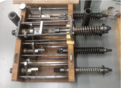
ADFEUP also owns a set of testing apparatus that use springs to apply tension to the specimens (Figure 2.10). The problem with these derives from Hooke’s Law: as the specimen is deformed, the spring’s length changes and so does the exerted force. Besides this, a mechanical indicator (Figure 2.11) is used to monitor the changes in the specimens’ length which requires manual readings and registry.

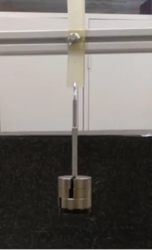
Because of the presented drawbacks, ADFEUP usually resorts to a simpler method when performing creep tests: to use weights attached to the specimen as the load appli-cation mean (Figure 2.12). The manual readings and registry are still required, but, as gravity doesn’t change, the exerted force on the specimens is constant.

(31)

2.4 Creep Testing Solutions in FEUP 11

Figure 2.9: An INSTRON 3300 series testing machine [18].

(32)

12 Literature Review

Figure 2.11: A mechanical indicator used to monitor changes in the specimens’ lenght.

Figure 2.12: Creep test using weights.

2.5 Discussion

Adhesive joints provide significant advantages over traditional joining methods and are increasingly drawing attention from the industry. Because of this, further study of this materials is required, especially regarding the creep phenomena.

As the defining characteristic of creep is time dependency, creep tests are usually lengthy. Besides this, the commercial offer of machines dedicated to this kind of testing is very limited: most multi-station test machines allow for independent tests but only under the same loading conditions, there are no multi stations machines dedicated to adhesive joints testing and the machines available are exceedingly costly. Because of this, manual testing is often the option taken to spare expensive testing machines for other kinds of research.

For these reasons, a multi-station machine dedicated to creep testing would be a valu-able asset to ADFEUP: not only would it spare the labour associated with manual test-ing but also allow more precise results and confident data, without any interference with other running projects. By developing and manufacturing this machine in FEUP, not only can we tailor it specifically to ADFEUP’s needs but we are also able to save significant amounts of money compared to the costs of acquiring a commercial machine with similar capabilities.

(33)

Chapter 3 Hardware

This chapter addresses the machine hardware. The solutions proposed in previous dis-sertations are analysed and the implemented alterations are explored. The chapter is split into three sections: Mechanical Design, Pneumatic Circuit and Electric Circuit. Each, in turn, addressing two topics: the proposed and the revised hardware.

3.1 Mechanical Design

Pina [5] revised the work of Freire [4] on the machine design, carrying out significant changes and improvements.

Pina’s machine (Figure 3.1) consisted of 6 mechanical wedge action grips (1), as-sembled in pairs, forming 3 testing stations.

The upper assembly (2), contains the 3 upper grips, the 3 load cells, the upper cou-plings between each of these sets, each ending in an axial spherical plain bearing, and all the necessary connections between these elements.

The lower assembly (3), contains the 3 pneumatic cylinders and their connections to the lower grips and to the lower beam. Both Freire and Pina planned for a future installation of a Climatic Chamber, encapsulating the testing zone and so, precautions were taken into account to negate its possible undesired effects on the functioning of the machine, namely assuring that the pneumatic cylinders were adequately spaced from extreme temperature sources and that all the materials would resist a broad temperature spectrum (which by ADFEUP specifications will range from −100◦C to +200◦C).

The machine structure (4) consists of a test frame formed by an upper beam and a lower beam, connected by two columns. This frame is assembled on top of a support frame which sustains the entire machine.

(34)

14 Hardware

Figure 3.1: Pina’s creep test machine mechanical design [5].

With the exception of some connecting parts, such as missing screws and bolts, most mechanical components of the machine were already manufactured as per Pina’s design. All except the heat sink, which becomes only relevant when the climatic chamber is im-plemented - which falls out of this dissertation’s objectives - and the extension springs, which pull the jaw faces of the grips against the shoe (Figure 3.2), allowing for the proper placement and tightening of the specimens. The springs are designed as described in the follow-up.

Figure 3.2: Grips’ jaw faces extension springs [5].

At their rest position, the springs have to ensure that the jaw wedges are as far apart as possible, allowing for maximum grip opening in that state. For this reason each set

(35)

3.1 Mechanical Design 15 of two springs has, in the aforementioned state, to counteract the weight of a jaw face wedge. Each wedge has a mass under 250 g, which results in an approximate weight of 9.81 × 250 = 2.45 N.

The centres of the screws holding the springs in place are 42.3 mm apart when the grip is at its maximum opening, and 49.3 mm when it is fully closed without any specimen between the jaw faces. These screws are ISO 4762 M4×12 screws, meaning that their 4 mm diameter has to be taken into account when choosing the springs, as the following scheme shows (Figure 3.3):

Figure 3.3: Grips’ jaw faces springs minimum (left) and maximum (right) extension. An extension spring stiffness, k, can be calculated by

k= 1 8

d4G nDm3

(3.1) where d is the nominal diameter of the spring wire (mm), G denotes the shear modulus of elasticity (N/mm2), n is the number of active windings and Dmrepresents the coil mean

diameter (mm) [20].

The company Fanamol, uses Inox AISI 302 steel, which has a shear modulus of 70.3 kN/mm2, to manufacture springs. Iterative calculations with the available springs led to a spring with the following characteristics: n = 28, Dm= 7 mm, d = 1 mm, L0= 44 mm.

The parameter L0being the undeformed length of the part.

Considering a linear spring behaviour, according to Hooke’s Law, the force, F, re-quired to extend (or compress) a spring is directly proportional to its extension, δ :

F= −kδ (3.2)

being k, the spring’s stiffness, a constant factor.

Through Equations 3.1 and 3.2, a minimum force of 2.1 N, when the spring is at its rest position, and a maximum force of 8.5 N, when the jaws are fully closed, can be determined. These values, the lower one being almost two times the required minimum

(36)

16 Hardware force, make allowance for some eventual loss of spring elasticity due to the effects of time and repetitive use.

Upon machine assembly, a severe design overlook was discovered. With the cylinders fully extended, there is a gap of roughly 170 mm between each set of upper and lower grips. ADFEUP’s specimens usually do not exceed 70 mm, most of them being consid-erably shorter. To mend this problem an extension to the upper coupling was designed. Ease of fabrication and integration with the already produced components was prioritized. The extension rod devised (Appendix A.1) is a simple φ 40×200 cylinder with threaded ends projected to assemble, without the need of additional parts, between the upper cou-pling and the load cells. It is manufactured in the same steel as the upper coucou-pling (AISI 304 austenitic stainless steel) to negate the effects of temperature variations due to the climatic chamber operation.

3.2 Pneumatic Circuit

Pina [5] proposed a pneumatic circuit including an air treatment unit feeding three pres-sure lines, each with a proportional prespres-sure regulator valve, a directional valve, a cylin-der, two flow control valves and two proximity sensors.

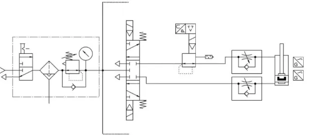
Figure 3.4: Pina’s pneumatic circuit proposed scheme [5].

The sugested pneumatic circuit scheme (Figure 3.4) shows only one of the stations as the remaining two are identical, after the air treatment unit. The suggested pneumatic

(37)

3.2 Pneumatic Circuit 17 circuit was adopted with a minor alteration (discussed in more detail in subsection 3.2.7) and some specific components replacement.

At the starting point of this dissertation the proportional pressure regulator valves and the cylinders had already been acquired by ADFEUP, as selected by Pina.

3.2.1 Cylinders

The chosen means to convert the power available in FEUP’s compressed air network in the form of pressure into the forces needed to perform creep tests were three Festo DDPC-Q-80-300-QA cylinders (Figure 3.5). These are standard cylinders with an integrated displacement encoder. They have a stroke of 300 mm and a φ 80 diameter piston with protection against rotation. Their working temperature can range from −20◦C to 80◦C. At 6 bar the cylinders can exert a theoretical advancing force of 3016 N and a theoretical retracting force of 2721 N. The cylinders are prepared for positioning sensing via external proximity sensors.

Figure 3.5: Pneumatic cylinders [21].

3.2.2 Pressure Regulator Valves

To control the pressure in the cylinders’ active chamber, and therefore the load applied on the specimen, one has to regulate it. This is achieved through the use of Festo’s VPPX-8L-L-1-G14-0L10H-S1 valves (Figure 3.6), from now on referred to as VPPX.

(38)

18 Hardware

Figure 3.6: VPPX [22]. Figure 3.7: VPPX schematic [22].

In Figure 3.7 a shematic of the VPPX valves is presented. The references in the next paragraph regard this image.

The VPPX valves have three connections to the pneumatic circuit: a supply port (1), a pressure output (2) and an exhaust port (3). The valves are designed to control pressure from 0.1 bar to 10 bar, having two operating modes: in the internal mode the valve uses an integrated pressure sensor at the pressure output and compares its signal (X ) to the setpoint value (W ), regulating the output flow to minimize the difference between these two; in the external mode the valve compares instead an external value (Xext) to the setpoint value

(W ).

We wanted to use the external control mode, feeding the valves the signal from the load cells, forcing them to regulate their pressure output according to the load measured and effectively regulating the load on the specimen. However it was only later realized that the valves had been supplied configured for internal mode operation and that, to change to external mode, one had to connect the valves to a computer and reconfigure the valves’ own software. This arose two possible courses of action: ADFEUP could buy the necessary special adapters to connect the valves to a computer and execute this procedure or could request an intervention by a FESTO technician. The latter option was chosen due to the costs associated with the first. Nonetheless, at the time of writing, said intervention had still not been made and so the VPPX valves are operating in internal control mode.

3.2.3 Air Treatment Unit

The MSB4-AGC:C4:H3:N3-WP Festo service unit (Figure 3.8) was selected instead of the one proposed by Pina, as the previously chosen model was unavailable. It is of equiv-alent characteristics, namely: an ON/OFF manual valve with silencer, a 5 µm filter

(39)

(rec-3.2 Pneumatic Circuit 19 ommended for the cylinders good functioning) with a plastic bowl guard, a manual con-densate drain, a pressure regulator ranging from 0.5 bar to 12 bar with a pressure gauge and regulator knob.

Figure 3.8: Air treatment unit [23].

3.2.4 Directional Valves

A solution using using 5/3 directional valves had been suggested by Pina [5]. However a specific valve had not been selected.

Festo’s VUVS-L25-P53C-MD-G14-F8-1-C1 directional valves (Figure 3.9) were cho-sen. These are in-line 5/3 directional valves. When not actuated they are reset by me-chanical springs to their closed mid-position. The 3 positions of the valve allow for the cylinders to move up (by allowing air flow (i.e. pressure) to the lower chamber of the cylinder and connecting the upper one to the exhaust), down (by doing the opposite) or to stand still, thanks to their closed center.

The valves are internally piloted, having a minimum piloting pressure of 2.5 bar and are solenoid-actuated. Their solenoid coils operate at 24 V DC. The valves’ size was chosen according to the size and flow rate of the, already purchased, cylinders and VPPX valves.

(40)

20 Hardware

Figure 3.9: Directional valves [24].

3.2.5 Flow Control Valves

Pina [5] also suggested the use of one-way flow control valves in each chamber to control the flow of the exhaust air. This serves several purposes: in the case of specimen rupture, the flow control valve on the cylinder’s lower chamber negates the rupture effects on the air supply lines (possible spikes in pressure, affecting tests taking place in the machine’s other stations) and the jerking motion of the cylinder itself; the meter-out design helps reduce stick slip, improving the motion of the cylinders and, by restricting the flow rate of compressed exhaust air, we are effectively regulating the piston speed [25].

Festo’s GRLA-3/8-QS-8-D one way flow control valves were selected (Figure 3.10). Their male G3/8 thread allows for direct assembly on the cylinders pneumatic ports and their L shape allows for the cylinders (with the flow control valves) assembly close by each other, directing the pneumatic tubing behind them. On the end not connected to the cylinder the valves have a push-in 8 mm connector. The valves’ flow restriction is adjusted via a screw.

(41)

3.2 Pneumatic Circuit 21

3.2.6 Pneumatic Accessories

Along with the main components of the pneumatic circuit, pneumatic tubing, connection and other kinds of acessories were needed to assemble the complete circuit. Table 3.1 resumes the used material which was acquired from Festo.

Table 3.1: Pneumatic accessories Identification Model Qty. Function

Silencer UC 1/4 9 Noise reduction at the exhaust ports. Distribution Manifold FR-4-3/8 1 Distribution of compressed air from 1

supply line into 3 outlets.

Push-in Fitting QS-3/8-8 6 Easy connection between G3/8 ports and the 8 mm tubing.

Push-in Fitting QS-1/4-8 15 Easy connection between G1/4 ports and the 8 mm tubing.

3.2.7 Implemented Circuit

As was already said, the VPPX allow for a control of pressure from 0.1 bar to 10 bar. Despite this, the directional valves need a minimum of 2.5 bar for their internal piloting to function and the valve be actuated.

As we are doing creep tests, our only interest is to control the pressure when the cylin-ders are applying tension on the specimens, i.e., when they are moving down. Because of this, it was decided to move each VPPX valve downstream from the directional valves, to the line feeding the respective cylinder’s upper chamber as depicted in Figure 3.11.

(42)

22 Hardware One could argue that it is desirable to also control the pressure in the cylinder’s active chamber when it is moving up. However, by restricting the exhaust air flow from the secondary chamber of the cylinders using the existing flow control valves we are able to limit their ascension velocity. Besides that, as the pressure regulator of the air treatment unit is regulated for 6 bar there is no danger for the cylinders (which can handle up to 12 bar) and not even for the load cells if the system were to fail in such way that the cylinders were exerting compressive forces on these at maximum pressure (the load cells maximum permissible load is about 1.5 times greater than such forces).

The new pneumatic circuit has been assembled and is fully functional. The air treat-ment unit and the distribution manifold have been adjusted to the lower support frame using standard M8 T-bolts and nuts. A support for the VPPXs and the directional valves has been manufactured according to the schematics in Appendix A.2, upon which they have been mounted.

3.3 Electric Circuit

The electric circuit was the hardware part that required greater intervention. Pina had started its assembly but had not completed it. Aside from the original electrical circuit schematics [5] there was no further documentation of the state of the circuit. On top of that, FEUP’s technician which had accompanied Pina’s work was not confident that the assembled part of the circuit was in line with said schematics.

Primarily, a thorough revision of the assembled circuit was carried out to ascertain both its (lack of) completion and its corroboration to the schematics. Secondarily, a re-vision of the schematics was made. Finally, the planned modifications were carried out and implemented. The circuit is now fully assembled and functional, with the exceptions specifically identified along this subchapter.

The first problem identified in Pina’s electric schematics [5] was related to his com-mand panel. The machine has three stations that should work independently from each other. In its normal operation, the user has to be able to run a test in a specific station, re-gardless of the remaining stations’ status - whether they are running other tests or standing idle.

Pina proposed a 4 position selector switch to toggle which station was being manually commanded by the user (to set up specimens for example): none, Station 1, Station 2 or Station 3. The problem with this was that the user could unintentionally activate the manual operating mode for a station running a test just by moving this selector switch. Another, more serious, problem would arise if a test was running on Station 2 and the

(43)

3.3 Electric Circuit 23 user needed to set up specimens in Station 1 and in Station 3. To change the manually controlled station from 1 to 3, the user would be forced to pass through the Station 2 position, changing this station’s behaviour from auto to manual and stopping the running test.

Faced with the costs of acquisition of new electric material to circumvent this problem, ADFEUP felt that there was no need for a physical command panel asides from a ON/OFF switch and an emergency button. It was so decided that all other commands would be given through the computer interface. Besides the two mentioned switches, a "Powered On" and an "Emergency" light indicators were assembled on the front side of the electric cabinet.

The other problems with Pina’s schematics were mostly related with signals compat-ibility between the various subsystems. For a better understanding of this, a schematic representation of a station’s components which interact with the electric circuit is now presented in Figure 3.12. In this schematic the arrows represent the flow of information between the various items. It is important to notice that the arrows can represent multiple signals, with different characteristics. The interacting components are further explored along the present chapter, detailing said communications needs and characteristics.

(44)

24 Hardware

3.3.1 Load Cells and Load Cell Transmitters

As was already said, the machine accommodates, in its upper assembly, three load cells. These are used to measure the forces to which the specimen is subjected. Each TS Load Cell (Figure 3.13) is directly connected to a TA 4/2 Analog Transmitter (Figure 3.14), both components were manufactered by AEP Transducers and had already been previously acquired by ADFEUP.

Figure 3.13: TS Load Cell [26]. Figure 3.14: TA 4/2 Analog Transmitter [27].

Each Transmitter powers the respective Load Cell and receives its signals, converting them. Its output is an analog voltage in the range ±10 V, where +10 V correspond to a tension load of 6000 N and −10 V to a compression load of the same magnitude. The transmitter behaves linearly between these two points, with a linearity error inferior to ±0.02 %. Besides this analog voltage output signal, the transmitter needs to be powered at 24 V DC [26, 27].

3.3.2 Encoders and Measured Value Converters

The cylinders have an integrated linear encoder. Their sinusoidal signals outputs are con-verted to a DC voltage, in the range 0.1 V to 9.9 V, using a DADE Measured Value Con-verter - from now on simply referred to as DADE - produced by Festo (Figure 3.15) and also previously acquired.

Similarly to the Load Cell/Transmitter set, the cylinders’ encoders directly connect to the DADE. This connection required however three SIM-M12-8GD-5-PU cables from Festo which had not been purchased. The cables were bought and the three connections are working as expected.

(45)

3.3 Electric Circuit 25

Figure 3.15: DADE Measured Value Converter [28].

As we are working with relative displacement encoders, the DADE needs to be ref-erenced whenever power is lost. An additional first commissioning calibration procedure is also required on its first use or if DADE’s memory has been reset. For this reasons, the DADE requires several connections besides analog voltage output and power supply. These connections to the electric circuit are summarized in Table 3.2.

Table 3.2: DADE’s connections to the electric circuit PIN Description Signal Type Voltage

1 +24 V power supply power supply 24 V 2 Measured Signal analog output 0.1 ... 9.9 V 3 Reference Output digital output 0 / 24 V 4 0 V Measured Signal analog output GND -5 Reference Input digital input 0 / 24 V 6 Calibration Input digital input 0 / 24 V 7 Ready Output digital output 0 / 24 V 8 0 V power supply power supply GND

-The first commissioning procedure is as follows [28]: Step 1 Switch on the operating voltage.

Step 2 Move the cylinder to the zero point of the work stroke. Step 3 Set the "Reference Input" for at least 0.5 s.

Step 4 Reset the "Reference Input" signal. As soon as the "Reference Output" is set, the reference point is saved.

Step 5 Move the cylinder to the end position of the work stroke. Step 6 Set the "Calibration Input" for at least 0.5 s.

(46)

26 Hardware Step 7 Reset the "Calibration Input" signal. As soon as the "Ready Output" is set, the

work stroke is saved permanently.

Once the first commissioning has been executed, the referencing procedure is achieved by completing steps 1 to 4. In this case, the "Ready Output" signal is set along with the "Reference Output" in Step 4 [28].

After the first commissioning, it is not expected that the DADE’s memories are reset. For this reason, after this procedure is completed, the "Calibration Input" terminal will not need to be connected any more. The "Ready Output" shall however be connected to the computer to prevent the cylinder’s use in the unlikely event of the DADE loosing its memory. In that case some manual hardware intervention would be necessary for repeating the first commissioning calibration procedure.

At the time of writing, the first commissioning procedure had been completed for Station 3 only for reasons further explored in this chapter.

3.3.3 Pressure Regulator Valves

Each VPPX valve is powered at 24 V DC, outputs an analog signal X , which results from internal pressure measurements, needs a setpoint value W and, when working in external control mode, also needs an external signal representing the measured pressured X_ext, as said in Subsection 3.2.2. The valves’ electric connections are now summarized in Table 3.3.

Table 3.3: VPPX’s connections to the electric circuit

PIN Description Signal Type Voltage 1 Digital communication no connection -2 +24 V power supply power supply 24 V 3 - Setpoint Value (W−)

analogue differential input 0 ... 10 V 4 + Setpoint Value (W+)

5 Digital communication no connection -6 Actual Value (X ) analogue output 0 ... 10 V 7 0 V power supply power supply GND -8 External Actual Value (Xext) analogue input 0 ... 10 V

3.3.4 Directional Valves’ Solenoid Coils

Each directional valve solenoid needs a 24 V signal to be activated. Six MSSD-EB plug sockets (Figure 3.16) were acquired from Festo and the wiring of said sockets was made

(47)

3.3 Electric Circuit 27 in FEUP to save costs of acquiring the plug sockets with the corresponding cables already connected.

Figure 3.16: MSSD-EB Plug Socket [29].

Each solenoid is activated by a relay triggered by a signal from the computer com-manding the machine. In Pina’s schematics [5], the solenoids responsible for the up movement of the cylinders were activated only by the command panel. As this was elim-inated, some relays were repurposed from the discarded circuitry to allow their activation via the computer output.

3.3.5 Travel Limit Switches

Pina had already suggested the use of magneto-resistive proximity sensors to act as travel limit switches [5]. Six SMT-8M-A-PS sensors (Figure 3.17) were acquired from Festo. These sensors are compatible with the cylinders and designed to be assembled in the T-solts on their body. They operate at 24 V, switching their normally open contact when the piston is sensed. The sensor cable has 3 wire connections: the power supply, the power supply ground and the output.

Figure 3.17: SMT Proximity Sensor [30].

Two sensors have been mounted in each cylinder, imposing a safe work stroke. When activated, each sensor triggers a relay, which blocks the corresponding directional valve from allowing more airflow into the relevant cylinder chamber.

Pina had proposed that only the lower limit sensors’ signals would be used in the computer yet it was found pertinent to use all six sensors’ signals. All corresponding electric connections have been made.

(48)

28 Hardware

3.3.6 Power Supplies

Most of the machine’s subsystems require a 24 V DC power supply to operate.

A MRD-100-24 Mean Well switched power supply had already been acquired - Power Supply 1 (PS1), Figure 3.18. It has a 24 V DC, 4 A output, and the standard single-phase 230 V AC input.

A second linear power supply - Power Supply 2 (PS2), Figure 3.19 - was acquired from BLOCK Transformatoren-Elektronik. The GLS 230/24-3 is a single phase, sta-bilised DC power supply. This device has a 24 V DC, 3 A output and was acquired to power the DADE, the VPPX valves and the load cell transmitters since linear power sup-plies are better for avoiding noise related issues in sensor signals. All the remaining systems requiring a 24 V DC supply are powered by PS1.

Figure 3.18: Power Supply 1 [31]. Figure 3.19: Power Supply 2 [32].

3.3.7 Data Acquisition Boards

As we are using a computer to command the machine, we must be able to generate and in-terpret most of the signals explored so far. In order to attain that, we use a Data Aquisition (DAQ) system. As defined by National Instruments, DAQ "is the process of measuring an electrical or physical phenomenon such as voltage, current, temperature, pressure, or sound with a computer" [33].

For the computer to be able to interact with the electric circuit, two DAQ boards had already been acquired: a NI6010 and a NI6703, both manufactured by National Instru-ments.

The NI6010 (Figure 3.20) is a multifunctional I/O device with 6 single line Digital Input (DI), 4 Digital Output (DO), 16 Analog Input (AI) and 2 Analog Output (AO) channels. Its analog input and output range is −5 V to +5 V.

(49)

3.3 Electric Circuit 29

Figure 3.20: NI6010 DAQ board [34].

The NI6703 (Figure 3.21) is an output device featuring 16 Analog Output channels and 8 digital channels that can act as inputs or as outputs. Its analog output range is 0 V to 10 V.

Figure 3.21: NI6703 DAQ board [35].

The digital signals of both devices, as standard in this kind of equipments, are 5 V signals.

As already exposed, in the electrical circuit we have 24 V digital (input and output) signals and analog signals with various ranges that do not correspond to the DAQ boards ranges. Because of that, most of these signals need conditioning.

Pina’s DAQ channel assignment had some mistakes and was, in many cases, consid-ered somewhat illogic. Besides this, there were many wrongly connected wires to the DAQ boards that did not match Pina’s schematics. Because of this all the DAQ channels were re-assigned from scratch and the corresponding wiring made. One significant aspect of this assignment is that, because we lacked digital input channels, six analog inputs

(50)

30 Hardware were used for the travel limit switches. On Tables 3.4 and 3.5 each DAQ used channels and the corresponding interacting system can be observed.

Table 3.4: NI 6010 used channels and interacting systems I/O Device Interacting System

Channel Pin System Description Pin Terminal AI GND 25

DADE 1 0 V Measured Signal 4 X12.5 DADE 2 0 V Measured Signal 4 X12.3 DADE 3 0 V Measured Signal 4 X12.1 AI 0 1 DADE 1 Measured Signal (Analogue) 2 X12.6 AI 1 21 DADE 2 Measured Signal (Analogue) 2 X12.4 AI 2 22 DADE 3 Measured Signal (Analogue) 2 X12.2 AI 3 5 VPPX 1 Analogue Output X 6 X10.3 AI 4 6 VPPX 2 Analogue Output X 6 X10.7 AI 5 26 VPPX 3 Analogue Output X 6 X10.11 AI 7 28 FDC1 Cyl. 1: Upper Prox. Switch BK X9.2 AI 8 20 FDC2 Cyl. 1: Lower Prox. Switch BK X9.4 AI 9 2 FDC3 Cyl. 2: Upper Prox. Switch BK X9.6 AI 10 4 FDC4 Cyl. 2: Lower Prox. Switch BK X9.8 AI 11 23 FDC5 Cyl. 3: Upper Prox. Switch BK X9.10 AI 12 25 FDC6 Cyl. 3: Lower Prox. Switch BK X9.12 AI 13 7 LCell 1 Load Cell 1: Transmitter V OUT X11.1 AI 14 9 LCell 2 Load Cell 2: Transmitter V OUT X11.2 AI 15 10 LCell 3 Load Cell 3: Transmitter V OUT X11.3 PFI 0/P0.0 13 DADE 1 Reference Output 3 X13.2 PFI 1/P0.1 32 DADE 1 Ready Output 7 X13.1 PFI 2/P0.2 33 DADE 2 Reference Output 3 X13.6 PFI 3/P0.3 15 DADE 2 Ready Output 7 X13.5 PFI 4/P0.4 34 DADE 3 Reference Output 3 X13.10 PFI 5/P0.5 35 DADE 3 Ready Output 7 X13.9 PFI 6/P1.0 17 DADE 1 Reference Input 5 X13.3 PFI 7/P1.1 36 DADE 2 Reference Input 5 X13.7 PFI 8/P1.2 37 DADE 3 Reference Input 5 X13.11 PFI 9/P1.3 19 PC EMER Emerg. Relay (PC) - PC EME

(51)

3.3 Electric Circuit 31 Table 3.5: NI 6703 used channels and interacting systems

I/O Device Interacting System

Channel Pin System Description Pin Terminal AO 0 (V) 34 VPPX 1 Analogue Input W + 4 X10.2 AO GND 0 68 VPPX 1 Analogue Input W − 3 X10.1 AO 1 (V) 66 VPPX 1 Analogue Input Xext 8 X10.4

AO 2 (V) 31 VPPX 2 Analogue Input W + 4 X10.6 AO GND 2 65 VPPX 2 Analogue Input W − 3 X10.5 AO 3 (V) 63 VPPX 2 Analogue Input Xext 8 X10.8

AO 4 (V) 28 VPPX 3 Analogue Input W + 4 X10.10 AO GND 4 62 VPPX 3 Analogue Input W − 3 X10.9

AO 5 (V) 60 VPPX 3 Analogue Input Xext 8 X10.12

P0.0 2 EMERG Emergency Button - X5.1 P0.1 3 DV 1 UP Directional Valve 1: UP - X8.2 P0.2 4 DV 1 DWN Directional Valve 1: DOWN - X8.6 P0.3 5 DV 2 UP Directional Valve 2: UP - X8.3 P0.4 6 DV 2 DWN Directional Valve 2: DOWN - X8.7 P0.5 7 DV 3 UP Directional Valve 3: UP - X8.4 P0.6 8 DV 3 DWN Directional Valve 3: DOWN - X8.8 D GND 36 - Signal Conditioning Boards GND -

-+5 V 1 - Signal Conditioning Boards +5 V -

-3.3.8

Signal Conditioning Circuits

A circuit board designed for digital conditioning already existed (Figure 3.22). This con-ditioning circuit has 16 channels that allow the conversion of digital signals between the computer and the corresponding 24 V interacting system. Half the channels for computer output (PC OUT) signal conditioning and half for computer input (PC IN) signal condi-tioning.

The PC OUT channels, when presented with a high signal in the terminal connected to the DAQ board, connect the corresponding pin of the 24 V interacting system to the ground terminal. This allows for relay triggering, for example, connecting one coil ter-minal to a power source, and the other to the PC OUT terter-minal. The circuit will only be closed when a high signal is given by the computer on the respective channel and so that is when the relay is activated.

(52)

32 Hardware

(a) front (b) back

Figure 3.22: Signal Conditioning Board 1.

The PC IN channels, when presented with a high signal in the terminal connected to the 24 V interacting system, output 5 V in the corresponding pin connected to the DAQ system.

This circuit board has revealed to be of low quality manufacturing. Although having been resoldered several times during the course of this work, some channels’ behaviour is still unreliable. In addition to this, the board does not have enough channels for the necessary digital signal conditioning and presents no analog channels.

A unique signal conditioning board, capable of doing all the needed signal conver-sions, was planned. As, at the time of this dissertation, said board could not be manufac-tured in FEUP with the desired characteristics, smaller, independent circuits manufacture and implementation was carried out for the remaining signal conditioning.

It is important to notice that this existing (unreliable) board was not replaced because it is expected, in the near future, that the fabrication of the desired board to do all the signal conditioning becomes possible in FEUP.

Pina already demonstrated that using a voltage divider to convert the 0-10 V analog signals from the DADE to a 0-5 V range would not cause any loss of resolution [5].

The VPPX control range is from 0 to 10 bar. The 16 bit resolution of the DAQ output for this system, working with its 0 V to 10 V signal, can be calculated by

10

216 = 0.000 15 bar (3.3)

As half of this is still vastly greater than the VPPX input resolution we have no loss of resolution here too.

(53)

3.3 Electric Circuit 33 As the Load Cell Transmitter output is from −10 V to +10 V, and the analog input range of the DAQ board from −5 V to +5 V, we also have to use a voltage divider here.

Two standard voltage dividers were manufactured acording to the shematics in Ap-pendix B (pages 18 and 19), have been connected to the system and are functioning as intended. Voltage Divider 1 (Figure 3.23) halves the tension of the signals from the DADE and from the Load Cell Transmitters and Voltage Divider 2 (Figure 3.23) does the same operation for the VPPX analog output signals.

Figure 3.23: Voltage Divider 1. Figure 3.24: Voltage Divider 2. Some signal conditioning was still needed for the remaining digital signals. As 24 V to 5 V (and vice-versa) conversion is a common need in electric circuitry nowadays, a commercial available solution was approached. Two DST-1R4P-N boards were acquired from the Chinese manufacturer Alzard Automation. Despite their very low cost and the fact that, when tested with a multimeter, the boards were showing the expected behaviour, when connected to the DADE, these boards would not function correctly for unknown reasons (insufficient drive current is a possible (not confirmed) explication).

A new schematic was designed for a in-house manufacturing of this new signal con-ditioning board (Appendix B, page 20). This new board (Signal Concon-ditioning Board 2) works slightly differently from the existing one, as the DADE requires not a connection to the ground to close the circuit but a 24 V signal in its digital inputs. It has four PC OUT and eight PC IN channels. In Figure 3.25 we can see a scheme showing a PC IN and a PC OUT channel of this new circuit.

This design was tested with identical components using a prototyping breadboard, borrowed from one of FEUP’s laboratories (Figure 3.26). Once proven that the board functioned as desired, the circuit for the needed signal conditioning was implemented

(54)

34 Hardware

(a) PC IN

(b) PC OUT

Figure 3.25: Signal Conditioning Board 2 Schemes.

on this breadboard for Station 3 only, pending the manufacturing of Signal Conditioning Board 2.

Figure 3.26: Prototype circuit.

Altough the components to manufacture Signal Conditioning Board 2 are relatively simple and easy to acquire (a standard matrix board, some terminal blocks, PCB sock-ets, optocouplers and resistances), the process for material funding and aqcuision is not. Because of this, it was not possible, up until the time of writing, to produce this board. Therefore, only Station 3 is functional.

(55)

3.4 Discussion 35 All the remaining electric circuit has been implemented and tested. All the wiring con-nections have been made and are ready to receive this missing board, upon installation of which the circuit will be fully functional. It is important to notice that it is still necessary to carry out DADE 1 and DADE 2 first commissioning procedures. In Figure 3.27 the cabinet containing the electric circuit can be seen.

Figure 3.27: Electric cabinet.

3.4 Discussion

Pina’s mechanical components of the machine have been assembled. Asides from some screws and bolts, the only missing parts were the grips’ springs, which have been calcu-lated and bought, and an extension rod (for each station), which has also been manufac-tured.

The missing pneumatic components were chosen and purchased. The pressure regu-lator valves were moved downstream from the directional valves because the latter have a minimum piloting pressure which would reduce the pressure regulation range unnecessar-ily. The entire pneumatic circuit has been assembled and tested, and it is fully functional. The physical command panel was eliminated. All commands to the station will now be given through the computer. A linear DC power supply was acquired to power the

(56)

36 Hardware DADE, the VPPX valves and the load cell transmitters. All the DAQ devices’ channels have been re-assigned and rewired. Two voltage dividers were manufactured to make possible the analog communications between the various systems and the computer. A digital signal conditioning board is pending fabrication, its design having been previously tested. A prototyping board is being used to make possible the operation of Station 3 while this digital signal conditioning board is not fabricated. All the remaining circuitry has been assembled and tested and it is fully functional.

(57)

Chapter 4 Software and System Behaviour

The machine is commanded and supervised by a computer. This chapter addresses the im-plemented software and simultaneously the system behaviour as they are intrinsically de-pendant on each other. Although some specific perks of the programming will be brought to attention, instead of dwelling into the details used to program the system behaviour, the software analysis will be mostly a functional one.

4.1 NI LabVIEW

LabVIEW (Laboratory Virtual Instrument Engineering Workbench) is a programming language developed by National Instruments.

Unlike the conventional programming languages, LabVIEW is a graphically based programming language. Every LabVIEW programming element, called Virtual Instru-ment (VI), has two main components, displayed in separate windows: a front panel and a block diagram. The front panel is where the controls and indicators are displayed, where the user interacts with the program. The block diagram is the source code of the VI. That is, the ambient which contains the programming behind the front panel to actually make it do something [36].

LabVIEW was chosen as the programming language because of two main reasons. The fist is that the DAQ boards were manufactured by National Instruments, and Lab-VIEW has VIs that facilitate the programming involving such boards. The second is that there is already other testing equipment used by ADFEUP programmed in LabVIEW, and so, the researchers of this group are already comfortable using this software.

Pina [5] made some suggestions regarding the Graphical User Interface (GUI) and experimented a bit with the front panel but did not program much on the block diagram. For this reason, his software would not accomplish anything on the hardware, and so it

(58)

38 Software and System Behaviour was not used. All the programming implemented in the machine was entirely developed by the author of the present dissertation.

4.2 System Behaviour Overview

The system was designed to work as an independent state machine for each station. Each state is the program waiting for something: for an event to be detected or actions to be completed. The events can be external to the coding (for example the activation of a relay) or internal (for example a timer inside certain state) [36].

Our machine has 8 possible states (for each station) that are briefly presented in Fig-ure 4.1. Every state acts as a diferent screen for the user to interact with and can contain multiple sub-states and actions. Each state’s behaviour and programming will be explored in detail along this chapter.

Figure 4.1: General station behaviour.

Because, at the moment of writing, only Station 3 is functional (as explained in Sec-tion 3.3) the program was only implemented for this staSec-tion. It was however developed with the three stations in mind and coded in a way that makes easy the implementation of the remaining two. For now, we will focus on Station 3, noting the required adaptations for the implementation of the software to the remaining stations along the way.

(59)

4.3 DAQ Assistant 39 Our main program runs inside a case structure nested in a while loop. The loop allows the code to run continuously, while the case acts as the "state" for our state machine. Every time the loop is ran, the code inside the active case is also ran. The input condition for the case structure is given via a shift register, this logs an output condition from the previous loop and feeds it as an input. In Figure 4.2 an example of this kind of structure is shown. In this case, the loop would run continuously in the "Awaiting Calibration" state, as the shift register (the blue symbol, with the arrow) is continuously being fed this value. Also inside this while loop, but outside the case structure we have the DAQ assistant tasks. These update local variables with the DAQ boards’ inputs or the DAQ boards’ outputs using local variables. Each local variable is associated to a control or indicator. Some of these for the user to interact with, others, hidden from the user, to merely function as auxiliary variables.

To make the program work with the two remaining stations, one would simply have to create a second and a third case structure inside the while loop; to associate these with two new, separate, shift registers; copy the code inside the implemented case structure to the new ones, changing variables accordingly (all local variables associated with Station 3 were coded with the prefix "ST3"). As new local variables have to be created, one simply has to change this prefix to refer to the appropriate station and add the new local variables to the DAQ assistant tasks, reconfiguring the latter accordingly.

Figure 4.2: A case structure nested in a while loop.

4.3 DAQ Assistant

LabVIEW has some built-in VIs to facilitate the programmer’s work. One of these is the DAQ Assistant Express VI. After a simple initial configuration (Figure 4.3) made through an assistant that LabVIEW automatically opens once we place the DAQ assitant block,

(60)

40 Software and System Behaviour the code for the acquisition of signals using DAQ boards is automatically generated and incorporated in a single block with simplified inputs and outputs.

The configuration includes the indication of which channels we are acquiring the sig-nals from, when we are acquiring them (every time the block is run, continuously at a fixed acquisition rate, or even just once), the voltage range of these signals, their terminal configuration and other parameters, like custom scaling and advanced triggering options.

Figure 4.3: DAQ assistant configuration window.

Because of the way LabVIEW runs its code, every DAQ assistant can only perform signal input or signal output. There cannot be multiple DAQ assistants, associated with the same DAQ board, executing similar tasks (i.e., reading AI, reading DI, writing AO or writing DO) and so, these must be combined in the same assistant. In Figure 4.4 we can see the DAQ assistants currently in use.

The first DAQ assitant handles the analog inputs connected to the NI6010 board. The block output is in the form of Dynamic Data (indicated by the thick blue line), this means that the data not only contains the voltage information but also time information. The

(61)

4.3 DAQ Assistant 41

Figure 4.4: DAQ assistant blocks and connections.

block connected to it is a Dynamic Data Converter. All it does is striping the time infor-mation from the data, outputting an array of voltages (thick orange line). Now we need to use an Index Array block to separate the elements of this array, because every one is a different analog input to the computer (orange thin lines). The first element is the mea-surement signal from the DADE. This analog voltage is converted using a custom Sub-VI created for the effect. Simply putting it, a Sub-VI is a program within a program. In this case all it does is the necessary arithmetic operations to convert the voltage signal from the DADE into millimetres. This value is then associated with the local variable ST3 DADE Measured Signal (mm). The signal from the analog output of the VPPX valves is numer-ically equal to half of the measured pressure in bar and so only needs to be mutiplied by two before its association with the local variable ST3 VPPX X (PIN 6). As we are using analog inputs for the travel limit switches, we are checking if the voltage is higher than 2 V and saving this logic value to the local variables ST3 FDC5 UPPER and ST3 FDC6 LOWER, respectively. To convert the voltage signal from the Load Cell Transmitter, one has to multiply this value by 600 (the load cell transmitter outputs 10 V with a load of 3000 N and 0 V at 0 N, behaving linearly between these points, but the voltage from the transmitter is being halved by Voltage Divider 1 before entering the DAQ board). The load cell value, in Newtons, is then associated to ST3 LCell (N).

The second DAQ assistant handles the digital input of the NI6010 board. Even though we only have one signal of this type, the block output is still an array of logic values (green thick line). The single existing element of this array still needs to be extracted with an Index Array block, after which it is linked to the ST3 DADE 3 Ref Output local

Development of a Three-Station Creep Machine for Adhesive Joints Testing

F

E

U

P

Development of a Three-station Creep

Machine for Adhesive Joints Testing

Eduardo Daniel Roque Silva

Integrated Master in Mechanical Engineering

Supervisor: António M. F. Mendes Lopes

Co-supervisor: Carlos M. S. Moreira da Silva

Co-supervisor: Lucas Filipe Martins da Silva

Development of a Three-station Creep Machine

for Adhesive Joints Testing

Eduardo Daniel Roque Silva

Integrated Master in Mechanical Engineering

Resumo

Abstract

Agradecimentos

Contents

List of Figures

List of Tables

Acronyms

Chapter 1

Introduction

1.1

Background and Motivation

1.2

Objectives

1.3

Methodology

1.4

Thesis Outline

Chapter 2

Literature Review

2.1

Adhesives

2.2

Creep

2.2.1

Creep Test Specimens

2.3

Commercial Creep Testing Mechines

2.4

Creep Testing Solutions in FEUP

2.5

Discussion

Chapter 3

Hardware

3.1

Mechanical Design

3.2

Pneumatic Circuit

3.2.1

Cylinders

3.2.2

Pressure Regulator Valves

3.2.3

Air Treatment Unit

3.2.4

Directional Valves

3.2.5

Flow Control Valves

3.2.6

Pneumatic Accessories

3.2.7

Implemented Circuit

3.3

Electric Circuit

3.3.1

Load Cells and Load Cell Transmitters

3.3.2

Encoders and Measured Value Converters

3.3.3

Pressure Regulator Valves

3.3.4

Directional Valves’ Solenoid Coils

3.3.5

Travel Limit Switches

3.3.6