The basis determinants: The European Case
Nuno Miguel Dias
Advisor: Joaquim Cadete
Dissertation submitted in partial fulfilment of requirements for the degree of Master in Finance, at the Universidade Católica Portuguesa
The basis determinants: The European Case
Abstract
With subprime mortgage crisis, Lehman Brothers Holdings Inc. bankruptcy and European government credit crisis, the CDS market assisted to a generalized turmoil, contributing for a decrease of CDS market in more than 50% in less than 3 years.
This dissertation focuses on testing possible determinants of the basis spread for several European companies, analysing data between June 18 2008 and December 31 2012. All financial information and data used in this thesis was gathered from Bloomberg.
Literature on single-name credit modelling and valuing credit derivatives is revised and applied to calculate the basis, with special focus on estimating hazard rates, where we used the optimization method instead of the generally used bootstrap method.
We than, followed Zhu work and analysed the proposed determinants for the basis, updating his work by introducing two new variables as potential determinants of the basis: the CDS Big Bang and the Lehman Brothers bailout.
Finally, we have found some evidence that efforts to standardize and regulate the credit derivative contracts, the CDS Big Bang has contributed to mitigate part of the counterpart risk, and that have also been reflected on the CDS-ASW basis.
This dissertation could not have been done without the direct and indirect support of several people.
I would like to express my gratitude to Professor Joaquim Cadete for the unconditional availability, superior knowledge and experience, promoting very high guidance and delivery necessary tools for the dissertation development and conclusion.
Special thanks to Professor Manuel Monteiro Leite for the review of statistics and econometric concepts.
Finally, I would like to deeply thank to Paula for never-ending love, support, and patience and dedicate this dissertation to her.
Abstract ... 2
Foreword ... 3
Table of Contents ... 4
INTRODUCTION ... 5
BACKGROUND THEORY ... 7
WHAT IS A CREDIT DEFAULT SWAP? ... 7
SINGLE-NAME CREDIT MODELLING –DEFAULT RATE STATISTICS ... 7
SINGLE-NAME CREDIT MODELLING –RECOVERY RATE STATISTICS ... 9
THE PRICING OF CREDIT DERIVATIVES ... 10
DERIVING THE DEFAULT SWAP PREMIUM USING ARBITRAGE ARGUMENTS ... 11
OBTAINING THE DEFAULT PROBABILITY ON A BINOMIAL MODEL ... 12
VALUING CREDIT DERIVATIVES USING STRUCTURAL MODELS ... 12
VALUING CREDIT DERIVATIVES USING REDUCED FORM MODELS ... 17
ANALYSIS FRAMEWORK ... 30
CREDIT DEFAULT SWAPS IN NUMBERS ... 30
THE EQUIVALENCE RELATION BETWEEN CDS AND BOND YIELDS ... 31
ESTIMATION OF RISK-NEUTRAL DEFAULT PROBABILITIES FROM CDS SPREADS ... 32
BUILDING A HAZARD RATE TERM STRUCTURE ... 34
ESTIMATION OF THE RISK-FREE RATES USING GERMAN TREASURIES ... 36
CALCULATING THE BASIS ... 36
DETERMINANTS OF BASIS SPREADS ... 39
DATA SET ... 41
EMPIRICAL ANALYSIS: THE DETERMINANTS OF THE BASIS BETWEEN CDS AND ASW SPREAD ... 43
CONCLUSION ... 48
1.1 APPENDIX –DATA ANALYSIS ... 49
1.2 REFERENCES ... 60
Introduction
Credit default swaps (CDS) have not only become the most widely used credit derivative, but have also turned into a journalistic buzz word due to subprime mortgage crisis in late-2000s and, more recently, due to European sovereign credit crisis.
These richness of events in the last 5 years, start to struggle the credit derivatives desks in major financial institutions in order to price their products. One of the major parameter to price a credit derivative is the spread, which represents the credit risk of a
name involved in the deal and it had no more logic. Subsequently, most of the products
could not be priced any longer, creating some discrepancies in their value and subsequently some arbitrage opportunities.
One of those arbitrage opportunities relied on taking advantage of the difference between the asset-swap spread and the CDS of the respective underline. This difference is called basis. In a market without any arbitrage opportunity the basis is expected to be zero, but recently this basis has moved deeply away from zero.
One of the most interesting papers regarding the basis determinants, where developed by (Zhu, 2006). Zhu analyses data between the years 1999 and 2002 and addresses two major concerns that have significant implications for financial regulators and risk managers. First, is credit risk equally priced between the derivatives market and the cash market? Zhu, refers this question as accuracy of credit risk pricing issue, where low financial transparency and the existence of asymmetric information between protection buyers and sellers leads to potential arbitrage of credit risk across markets. Second, which market reacts more rapidly to changes in credit conditions? This question, reports to price discovery efficiency of both markets, where traders could take potential gains from price differentials.
Using Zhu’s work, we have applied the same framework for the between years 2008 and 2012, but with the introduction of two new dummy variables: the Lehman Brothers bankruptcy (September 15 2008) and CDS Big Bang (April 8 2009).
With the Lehman Brothers bailout, it is expected that the basis move away from zero, hence the risk perception in the market players has worsen. On the opposite, with the CDS Big Bang, it is expected that the basis approximate more to zero, because after April 8 2009 where introduced changes in CDS contracts and conventions in order to make CDS more standardised and consequently to help central clearing of CDS trades, mitigating the counterpart risk.
With our investigation, we tried to bring new information for the bank’s derivatives desk, in order to contribute for the definition of the liquidity premia necessary to face future credit events. Thus, it is expected to answer the following questions: Does the Lehman Brothers bailout augment the risk perception? In which way affected the basis? Does the Big Bang event helped to mitigate the counterpart risk? How it influenced the basis? How does rating events and liquidity influence the basis?
Finally, unlike Zhu did in his paper, hazard rates are taken through the optimization process and not through bootstrapping method. The optimization method has the advantage of dealing with the liquidity of CDS quotes, putting more emphasis in liquid ones and less emphasis in illiquid maturities.
The rest of this thesis is structured as follows. Chapter 2 starts to briefly analyse the dimension of the credit derivative market, explain what is a CDS and introduces a theoretical background regarding the main models of CDS valuation. Chapter 3 explains in detailed the analysis framework used in this dissertation, including the relationship between the credit spreads in the bond market and the derivatives market from a theoretical perspective. Chapter 4 describes the data. Chapter 5 identifies the determinants of the basis. Chapter 6 concludes.
Background Theory
What is a Credit Default Swap?
The most important credit derivative is the credit default swap (CDS). This is a contract between two parties, where one party transfers to another the credit risk of a reference entity, corporate or sovereign, for a specific period of time. A CDS is designed to protect an investor against the loss from par on a bond or loan following the credit event of the reference entity, including bankruptcy, failure-to-pay and restructuring. In return for this, the protection buyer pays a premium to the protection seller.
There are also a number of option-based credit derivatives. These include single-name default swaptions in which the option buyer has the option to enter into a CDS contract on a future date. More recently, we have assisted to the growth of portfolio swaptions, where the holder has the option to enter into a portfolio of CDS. These contracts work by “tranching” up the credit risk of the underlying portfolio. Tranching is a mechanism by which different securities or tranches are structured so that any default losses in the portfolio are incurred in a specific order. The first default losses are incurred by the riskiest equity tranche. If the size of these losses exceeds the face value of the equity tranche then the remaining losses are incurred by the mezzanine tranche. If there are still remaining losses after this, then these are incurred by the senior tranches. The risk of this credit derivatives contract is sensitive to the tendency of the credits in the portfolio to default together. This is known as default correlation and, for this reason, these derivatives are known as correlation products.
An important extension of the CDS is the CDS index. This product allows the investor to enter into a portfolio consisting of 100 or more different CDS in one transaction, exposing the issuer to the default risk of more than one credit or “name”, we call this transaction multi-name product. The multi-name products have several advantages to
the single-name products, mainly considerable liquidity and diversification.
Lastly, we have the credit Constant Proportion Portfolio Insurance (CPPI) structure and the more recent Constant Proportion Debt Obligation (CPDO) structure. These structures exploit a rule-based dynamic trading strategy typically involving a CDS index. In the case of CPPI, it is designed to provide a leveraged credit exposure while protecting the investor’s principal. In the case of CPDO, the strategy is designed to produce a high coupon with low default risk. Due to the complexity involving the valuation of multi-named products, we will focus our thesis in single-named products. Single-name credit modelling – Default rate statistics
In order to define a model for pricing credit derivatives, we need to establish a modelling framework which can capture the appropriate risks, which includes default risk, recovery rate risk, spread risk, interest rate risk and credit rating transition risk. Default risk is the risk that a planned payment of interest or principal on a bond or loan
is not received. Recovery risk is the risk that following a default, the size of the recovered amount is less than the amount due. Spread risk is the risk that the value of a credit security falls as the market’s view regarding the credit quality of the borrower changes, causing us to realise a loss if we sell the credit security. Interest rate risk is the risk that changes in the level of the treasury curve will cause the value of the credit security to fall. Credit rating transition risk is the risk of credit note change of the reference entity or issuance.
Default is a complex event that can occur for several reasons. In some cases it is an entirely idiosyncratic event that strikes just one company. In other cases can be a systemic event in which several companies or sovereigns are all affected by the same factor.
The main sources of default statistics are the credit rating agencies. In order to better assess the issuers’ credit quality, they have collected a significant amount of data over their lifetime. In order to measure default, it is important to understand the default definition. According to Moody’s, a default is “any missed or delayed payment of interest or principal, bankruptcy or distressed exchange where,
(i) the issuer offered bondholders a new security or package of securities that amount to a diminished financial obligation (such as preferred or common stock or debt with a lower coupon or par amount), or
(ii) the exchange had apparent purpose of helping the borrower avoid default”. If a failure to pay principal or coupon occurs as a result of some omission, which is quickly rectified, then the event is known as technical default. Such an occurrence is not usually included in rating agency default statistics.
The rating agency methodology for calculating default statistics has been to construct databases of issuers and to monitor the dating and default behaviour of the senior unsecured bonds of each issuer through time. This is done by identifying a cohort – a group of issuers with the same initial rating. The rating agency then keeps track of the
cohort and records if any of the issuers default. As a result, it is possible to calculate the
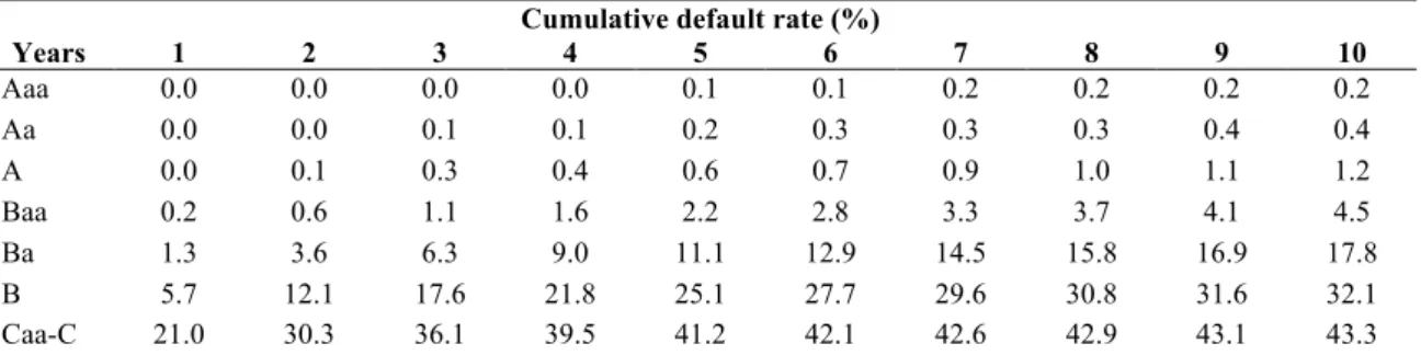
number of defaults in each cohort. Dividing this by the number of issuers in the cohort gives the average default rate of issuers with a specific rating. Each year new cohorts are defined. Averages can then be taken across cohorts with different initial dates but with the same initial rating to give a time-averaged default rate for each rating class. The next table shows time-averaged cumulative default rates and so has averaged out any time variability in default rate statistics. In practice, market participants will use these historical default rates as proxies for the default probabilities used within their credit risk models. This assumes that time-averaged historical default rates by rating are a good predictor of future default rates, and that all issuers with the same rating have the same probability of default. It therefore ignores the current state of the credit environment and differences in credit quality that exist within a rating category. The averages are global, so that differences in the triggering of default and the workout process which may exist across different legal jurisdictions are not captured. The data is
also biased towards US corporate credits since this has traditionally been the dominant market for corporate credit bonds. However, this issue is now being addressed by the rating agencies that have recently begun to produce separate statistics for the European credit market.
Figure 1 Average cumulative default rates of corporate bond issuers by letter rating from 1983 to 2005 Cumulative default rate (%)
Years 1 2 3 4 5 6 7 8 9 10 Aaa 0.0 0.0 0.0 0.0 0.1 0.1 0.2 0.2 0.2 0.2 Aa 0.0 0.0 0.1 0.1 0.2 0.3 0.3 0.3 0.4 0.4 A 0.0 0.1 0.3 0.4 0.6 0.7 0.9 1.0 1.1 1.2 Baa 0.2 0.6 1.1 1.6 2.2 2.8 3.3 3.7 4.1 4.5 Ba 1.3 3.6 6.3 9.0 11.1 12.9 14.5 15.8 16.9 17.8 B 5.7 12.1 17.6 21.8 25.1 27.7 29.6 30.8 31.6 32.1 Caa-C 21.0 30.3 36.1 39.5 41.2 42.1 42.6 42.9 43.1 43.3
Source: Hamilton et al. (2005).
Historical default data is not used by the market for determining the price of a security. It is primarily used as a way of calibrating risk models. When we come to pricing credit risky assets such as credit derivatives, we need to be in a world in which we can hedge out the risk that these contracts present. For that, we need to be in a risk-neutral framework.
Single-name credit modelling – Recovery rate statistics
Credit risk is also about the risk associated with the amount of the claim that can be recovered after default. In the credit derivatives market, the recovery price is the price of some reference obligation determined within 72 days of the default event. The measure of recovery rate used in the credit markets is the defaulted bond price divided by the face value. There are a number of sources for recovery data. In our study, we will a recovery rate of 40% of the face value. This value, is used as general accepted in most models of CDS valuation, and is based on the study performed by Altman et al. (2003b). In this study, it is empirically estimated recovery rates based on prices just after default on loans. The following table resumes the findings:
Figure 2 Empirical estimates of recovery rates
Seniority of debt Debt type Number of
issues Median recovery (%) Mean recovery (%) Standard deviation (%)
Senior secured Loans 155 73.00 68.50 24.4
Senior unsecured Loans 28 50.50 55.00 28.4
Senior secured Bonds 220 54.49 52.84 23.1
Senior unsecured Bonds 910 42.27 34.89 26.6
Senior subordinated Bonds 395 32.35 30.17 25.0
Subordinated Bonds 248 31.96 29.03 22.5
All bonds and loans 1909 40.05 34.31 24.9
The pricing of credit derivatives
The pricing of credit derivatives is not an easy task. One of the major reasons is that the market price of the underlying asset is not often easily observable. This is particularly applicable for loans, which are rarely traded in a secondary market. Nevertheless, if the underlying company is rated by an agency, the rating can be used as a proxy to value the respective debt, but published ratings are often outdate, since agencies are not able to analyse the underlying debt on a timely basis, and defaults are rare events. Especially, since a company typically only defaults once, empirical data on the default of a solvent company is typically unavailable.
In addition, default is usually triggered by a combination of factors, like as credit, market and operational risk, whose correlation has to be integrated into the pricing model. Moreover, with credit derivatives, the counterparty risk is an important pricing element, since the default of the underlying debt typically leads to a large settlement payment of the protection selling counterparty. Ideally, the correlation between the default risk of the counterparty and the default risk of the underlying debt should be considered in the pricing process. All this makes pricing credit derivatives complex. Lastly, there is no pricing model generally accepted as a benchmark as, for example, the Black-Scholes model for standard options. Additionally, incorporating all input variables, summarized in the next table, it is not trivial.
Figure 3 List of variables for valuing a credit derivatives price Input for deriving the price of a credit derivative
1) Default probability and credit deterioration probability of the reference asset 2) Default probability and credit deterioration probability of the credit derivatives seller 3) Correlation between 1) and 2)
4) Volatility of the underlying reference asset 5) Volatility of the credit derivatives seller 6) Correlation between 4) and 5)
7) Maturity of the credit derivative
8) Expected recovery rate of the reference asset 9) Expected recovery rate of the credit derivatives seller
10) Return of the reference asset (e.g. coupon of the reference bond) 11) Risk-free interest rate term structure used to discount future cash-flows
12) Default probability of the credit derivatives buyer in case of periodic credit derivative premium 13) Expected recovery rate of the credit derivatives buyer in case of periodic credit derivative premium 14) Correlation between de default probability of the credit derivatives buyer and the reference asset in case of
periodic credit derivatives premium
15) Market risks (as interest rate risk, currency risk, commodity risk, and stock price risk) and the correlation between market risk and credit risk
16) Operational risks (e.g. legal risks, documentation risks, or settlement risks), which might endanger the enforceability of the payoff and the correlation between operational risk and credit risk
18) Liquidity of the underlying reference asset 19) BIS risk weight on the credit derivatives seller
20) Urgency of protection (e.g. in an immediate credit deterioration expected or does the protection free up credit lines to enable further business with a client)
21) Transaction costs
Source: (Meissner, 2005)
Furthermore, the credit risk models can be divided into two major groups, the structural
models and reduced form models (also known as intensity-based models). The structural models were pioneered by (Merton, 1974), in his framework a firm issues two
types of assets: equities and bonds. A default occurs if the total asset value falls below a default boundary, this is a level of asset value, sufficiently low so that the firm decides to default on its debt if asset value falls beneath this level. By contrast, reduced form
models treat default as a random stopping time with stochastic arrival intensity. The
credit spread is determined by risk neutral valuation under the absence of arbitrage opportunities. This method has been widely used in the pricing of CDSs, the main literature was developed by (Jarrow & Turnbull, 1995), (Das, 1995), (Duffie, 1999), (Duffie & Singleton, 1999), (Das & Sundaram, 2000), (Madan & Unal, 2000), (Hull & White, 2000, 2001), (Archarya, et al., 2002), (Jarrow & Yildirim, 2002), (Das, et al., 2003) and (Schönbucher, 2003).
Before we discuss structural and reduced-form models in detail, is important to understand simple pricing features of credit derivatives, namely the default swap
premium derived from asset swaps, deriving the default swap premium using arbitrage arguments and obtaining the default probability on a binomial model.
Deriving the default swap premium using arbitrage arguments
An important arbitrage argument, used in trading practice to help determine the price of a default swap can be expressed in the following terms:
Default swap premium = Return on risky bond – Return on risk-free bond. (1)
This equation can only serve as an approximation, hence it abstracts from several inputs, already described, which have to be included in the pricing of a default swap. One of the most important points, not included in the previous equation, is the counterparty risk, this is the risk that the default protection seller defaults. In addition, the correlation between counterparty default risk and default risk of the underlying asset assumes also a degree of importance, since the default protection buyer will incur a loss in the amount of his reference asset value plus the default swap premium (minus the recovery rate of the reference asset issuer and the counterparty), if both the protection seller and the underlying asset default.
Obtaining the default probability on a binomial model
One of the most important features when pricing credit derivatives is deriving the probability of default of the underlying debt.
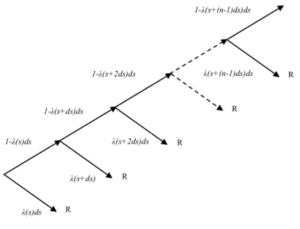
We can model the default in a one-period setting as a binomial tree, which we survive with probability 1- λ(s)ds or default and receive a recovery value R with probability
λ(s)ds. For a n-period, the risky debt with a notional amount of 1, can be designed as
follows:
Figure 4 Binomial model to find the risk-neutral probability of default
Risk-neutrality is an important concept when pricing derivatives. If investors are risk-neutral, they do not require a compensation for taking risk. As a consequence, the expected return on all securities (including derivatives) is the risk-free interest rate. Hence, the present value of any security can be derived by discounting all future cash flows with the risk-free interest rate.
Valuing credit derivatives using Structural Models
As we have presented earlier, structural models derive the probability of default by analysing the capital structure of a firm, especially the value of the firm’s assets compared to the value of the firm’s debt.
The original 1974 Merton model
In 1974 Robert Merton created a firm value model to estimate a company’s value of debt and the probability of default (Merton, 1974).
R R R R R λ(s)ds λ(s+ds) λ(s+2ds)ds λ(s+(n-1)ds)ds 1-λ(s+(n-1)ds)ds 1-λ(s+2ds)ds 1-λ(s+ds)ds 1-λ(s)ds
The Merton call
Merton combined the simple equation, shareholders’ equity (E) = company’s assets (V) – company’s liabilities (D), with the Black-Scholes option pricing framework. Merton’s model is mathematically identical with the original Black-Scholes equation for valuing a call: E0 = V0N(d1) – De-rTN(d2) (2) where 𝑑! = !" !! !!!!! ! ! !!!!! !! ! and 𝑑! = 𝑑!− 𝛿! 𝑇
where E0 is the current value of equity, V0 is the current value of assets, D is the debt to be repaid at time T, N is the cumulative standard normal distribution, r is the risk-free continuously compounded interest rate, 𝛿! is the expected volatility of the asset, and T is the option maturity, measured in years. The previous equation states that equity holders have a claim on the assets of a company: If the asset value V increases, the equity value E will increase with unlimited upside potential; on the downside, it the debt
D exceeds the assets V, the company will go bankrupt. In this case the equity holders
will take the remaining assets to repay part of the debt, the equity value being zero. A well-known property of the Black/Scholes model is that the risk-neutral probability of exercising a call option is N(𝑑!). Therefore, the probability of not exercising the option is N(−𝑑!). Not exercising the equity option means that the debt D is bigger than the assets V. This is the case of bankruptcy. Therefore, the probability of default in the Merton framework is N(−𝑑!).
The Merton put
The value of credit risk and the probability of a company’s default in Merton’s model can also be found by expressing credit risk with the help of a put option on the assets of the company: The equity holders can hedge the credit risk by buying a put on the assets with strike D, the put seller being the asset holders. In case of default, i.e. V < D, the equity holders will deliver the assets to the asset holders, the loss for the asset holders being D – V. Thus, the put option can be expressed as in the following equation:
𝑃! = −𝑉!𝑁 −𝑑! + 𝐷𝑒!!"𝑁(−𝑑 !) (3) where 𝑑! = !" !! !!!!! ! ! !!!!! !! ! and 𝑑! = 𝑑!− 𝛿! 𝑇
where 𝑃! is the current value of a put option on the company’s assets V with strike D, σ is the volatility of the underlying asset, and T is the option maturity expressed in years. The equity holders will exercise the put option in the last equation at time T if D > V. In the Merton model, this is the case of bankruptcy. Thus the probability of exercising the put, which is 𝑁(−𝑑!), is again the probability of default.
Rewriting the previous equation as 𝑃! = −! !!!
! !!! 𝑉!+ 𝐷𝑒
!!" 𝑁(−𝑑
!) results in an intuitive interpretation of the default risk, where the term ! !!!
! !!! 𝑉! reflects the amount retrieved of the asset value 𝑉! in case of default, thus the recovery value. The term 𝐷𝑒!!" is the present value of the debt, thus −! !!!
! !!! 𝑉!+ 𝐷𝑒
!!" is the present value of the loss in the event of default. Multiplying −! !!!
! !!! 𝑉!+ 𝐷𝑒
!!" with the probability of default 𝑁(−𝑑!) gives the present value of the default risk, which equals the put value 𝑃!.
The put option in equation (3) serves as a basis to find a closed form solution for the value of the underlying risky bond B. We can start by expressing 𝐵! as the debt D to be repaid at time T discounted by 𝑒!!" minus the value of the credit risk, which is the put in equation (3):
𝐵! = 𝐷!𝑒!!"− −𝑉
!𝑁 −𝑑! + 𝐷𝑒!!"𝑁(−𝑑!) (4) Rearranging the equation and assuming 1-N(-𝑑!)= N(𝑑!) results in the value of the risky bond of:
𝐵! = 𝐷!𝑒!!"𝑁 𝑑 ! + 𝑉𝑁(−𝑑!) (5) Where 𝑑! = !" !! !!!!! ! ! !!!!! !! ! and 𝑑! = 𝑑!− 𝛿! 𝑇
One drawback of Merton’s model is that we need the asset value V and the asset volatility 𝛿! as inputs. Both parameters are not easily available in practice. However the equity value E and the equity volatility 𝛿! are observable. Using equation (2) and equation (6) derived from Itô’s lemma:
𝐸! =! !!!!!!!
! (6)
We have two equations with two unknowns to solve for, V and 𝛿!.
As mention earlier, the Merton model serves as a basis for structural and reduced form models that value credit risk. Meanwhile, the model simplifies a number of aspects. It principally only allows default at the maturity of the debt T and the debt can only take the form of zero-coupon bonds. Coupons as well as different seniorities cannot be
handled. There is only one bankruptcy event, which occurs when the asset value falls below the value of the debt at maturity of the debt. Other bankruptcy event such as illiquidity, restructuring of debt, or a moratorium is not taken into account.
Nevertheless, the Merton model has served as an excellent basis for developing more realistic complex models.
The Black-Cox 1976 model
(Black & Cox, 1976) suggest an exogenous exponential default boundary with two exogenous constants, k and γ. If the asset value drops below the default boundary during a period of time, the asset holders can force the company in to bankruptcy or restructuring. The mandatory bankruptcy or restructuring, expressed as a safety
covenant of the asset holders, is an important feature of the model. It protects asset
holders from further deterioration of the company’s assets. In that sense a high value of
k and a low value of γ forces early bankruptcy or restructuring and principally protects
asset holders.
Besides safety covenants, Black and Cox also investigate subordination arrangements and restrictions for the equity holders to finance interest and dividend payments. All three provisions tend to increase the value of the risky bond.
Black and Cox also find a closed form solution for the risky bonds, which includes (continuous) dividends to the stockholders and the underlying interest rate process and the recovery rate are rather simple. Interest rates do not follow a stochastic process but are assumed constant at a constant rate and the recovery rate is simply set to the asset value at the time of default.
The Kim, Ramaswamy, and Sundaresan 1993 Model
(Kim, et al., 1993) use a simpler default boundary but a more realistic stochastic interest rate process than Black and Cox. Default is triggered if the asset value drops below a exogenous constant variable. The interest rate process follows the risk neutral Cox-Ingersoll-Ross model, where interest rates mean-revert with a defined rate to the long-term average of rates. These rates cannot get negative, because are taken to the square root.
The default boundary in this model takes into account the coupon rate and the cash outflow of the firm. Thus the default boundary is endogenous but not time-dependent as in the Black-Cox model. The recovery rate is the minimum of the asset value and the face value of the debt, if default occurs before the debt maturity, the recovery rate is the minimum of an exogenous recovery rate expressed in percentage of a risk-free bond and the asset value.
According to the authors of the study, this model had better results in deriving realistic default swap premiums than the original Merton model.
The Longstaff-Schwartz 1995 model
(Longstaff & Schwartz, 1995) suggest a first-time passage model with an exogenous and constant default boundary and recovery rate. For the interest rate, Longstaff and Schwartz use the Vasicek1 model.
With the help of the closed form solution for a zero-coupon bond derived in the Vasicek model, Longstaff and Schwartz find a solution for the price of risky zero-coupon bonds and floating rate bonds.
Key findings of Longstaff and Schwartz imply that credit-spreads decrease when the risk-free Treasury rate increases. This appears counterintuitive but can be explained by the fact that a higher interest rate means a higher growth rate of the asset value. As a consequence of the higher asset value the probability of default is lower, and with it the credit-spreads.
The inverse relationship between long term risk-free interest rates and credit-spread is stronger for firms with lower credit quality. This is intuitive since a strong growth in the asset value can improve the asset-liability relationship of a low rated firm to a significant degree.
Drawbacks of the Longstaff-Schwartz model are the complex parameter calibration of the numerous parameters for the bond equations, and the fact that the underlying Vasicek model for interest rates is generally not arbitrage-free.
The Briys-deVarenne 1997 model
In 1997, (Briys & Varenne, 1997) addressed shortcomings of the Black-Cox, Kim-Ramaswamy-Sundaresan, and Longstaff-Schwartz models. In these models, the payoff to bondholders in case of bankruptcy may be larger than the firm’s asset value. In this respect, payoff demands of the equity holders are not taken into account. Consequently, Briys and de Varenne suggest a default boundary and recovery rate, which guarantee that the payoff to bondholders at the time of default is realistic with respect to demands from the equity holders, and cannot be higher than the firm’s asset value.
Critical appraisal of structural models
The major achievement of the models presented is that unlike in the original Merton model, default before the maturity of the debt at time T is possible. However, several
significant drawbacks remain. First, with the exception of the Kim-Ramaswamy-Sundaresan model, the default boundary involves an exogenous constant. Furthermore, the recovery rate of the models, with the exception of the Black-Cox model, also involves an exogenous constant. Consequently the default boundary and recovery rate are difficult to determine for practical purposes.
In addition, the closed form solutions for the risky bond price, equations of the four last models are quite complex and the calibration of the numerous parameters to match market credit-spreads is difficult in trading practice. Other shortcomings of structural models include the fact that some underlying stochastic processes for the asset value (e.g. CIR2 and Vasicek) are generally not arbitrage-free. Altogether, these drawbacks have so far limited the use structural models in credit risk practice.
Valuing credit derivatives using Reduced form Models
They are called reduced form, since they abstract from the explicit economic reasons for the default, i.e. they do not include the asset-liability structure of the firm to explain the default. Rather, reduced form models use debt prices as a main input to model the bankruptcy process. Default is modelled by a stochastic process with an exogenous
default intensity or hazard rate, which multiplied by a certain time frame, results in the
risk-neutral default probability, also called pseudo-or martingale3 default probability. The value of hazard rate is derived by calibration of the variables of the stochastic process. Since reduced form models only model the timing of the default not the severity, the recovery rate is usually exogenous.
The Jarrow-Turnbull 1995 model
(Jarrow & Turnbull, 1995) were one of the first to derive the value of credit derivative and to price credit derivatives in the arbitrage-free reduced form model environment. They combine a process for risk-free interest rates and a bankruptcy process of the risky debt to derive default probabilities and credit derivatives prices. The two processes are assumed to be independent from each other.
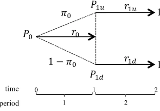
Let’s define P as the price of the risk-free zero-coupon bond with notional amount 1 and maturity at time 2. 𝜋! is the risk-neutral probability of an interest rate increase. This brings us to the following interest rate tree:
Figure 5 Risk-free interest rate tree in the Jarrow-Turnbull model
2 Cox–Ingersoll–Ross model (or CIR model) describes the evolution of interest rates.
Where r = risk-free interest rate, P = risk-free zero-coupon bond price
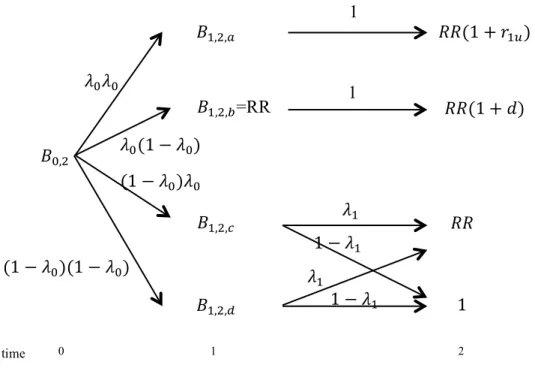
Figure 6 Bankruptcy process of risky bond B in the Jarrow-Turnbull model
The risk-free bond price at time t with maturity T, is Pt,T = 1/ (1 + rt,T). Since r1u > r1d, it follows that P1u > P1d.
Let B be the price of a risky zero-coupon bond with a notional amount of 1 and maturity at time2. Let λ be the risk-neutral probability of default, (1-λ) the risk-neutral probability of survival, and RR the recovery rate in case of default. Thus, we derive the default process for the risky bond B, in the Figure 6
Combining the last two figures, we get the following quadruple tree: 𝑃! 𝑃!! 𝑃!! 𝜋! 1 − 𝜋! 𝑟! 𝑟!! 𝑟!! 1 1 time period 0 1 2 1 2 time period 0 1 2 1 2 𝐵! 𝑅𝑅 𝜆! 1 − 𝜆! 1 𝜆! 1 − 𝜆! 𝑅𝑅
Figure 7 A combined interest rate and bankruptcy process
The unique, risk-neutral or pseudo-probabilities λ and π guarantee that the prices P and
B are martingales, this means that past events doesn’t help to forecast the future, thus
the model is arbitrage-free. Furthermore, the Markov4 property allows displaying the combined interest rate and bankruptcy tree as a recombining tree. They also use a foreign exchange rate analogy to model the risky bond price B. The risky bond price at any time t with maturity T, Bt,T, is equal to the risk-free bond price Pt,T multiplied with the “exchange rate” e, which is 1 in case of no default and equal to the recovery rate RR in case of default. Thus Bt,T = Pt,T et. If E(eT) is the expected payoff at time T, the risky bond price can be expressed as:
𝐵!,! = 𝑃!,!𝐸(𝑒!). (7)
The previous equation states that the risky bond price is the expected payoff E(eT) discounted by the risk-free price Pt,T.
The shortcomings of the Jarrow-Turnbull 1995 model lie in the basic approach of the model: the direct economic reasons for default, i.e. the company’s specific asset-liability structure or the company’s liquidity are not part of the analysis. Rather, bond prices are the major input, assuming that bond prices can serve to reflect the credit risk of the debtor and to derive default probabilities. However, it has been shown that bond prices overestimate a company’s probability of default quite substantially (Altman, 1989). In addition, bond prices are often illiquid, resulting in difficulties in determining a fair mid-market price.
4 A stochastic process has the Markov property if the conditional probability distribution of future states of the process depends only upon the present state, not on the sequence of events that preceded it.
time 0 1 2 1 𝜆!𝜆! 𝑅𝑅(1 + 𝑟!!) 𝐵!,! 𝐵!,!,! 𝐵!,!,!=RR 𝐵!,!,! 𝐵!,!,! 𝜆!(1 − 𝜆!) (1 − 𝜆!)(1 − 𝜆!) 𝑅𝑅(1 + 𝑑) 1 𝑅𝑅 1 𝜆! 1 − 𝜆! 1 − 𝜆! (1 − 𝜆!)𝜆! 𝜆!
Additionally, it is assumed that the interest rate process and the default process are independent. Also, the default intensity is assumed constant, thus default is equally likely over the life of the debt. Last, the recovery rate of the model does not depend on the model variables, but is exogenous.
These shortcomings were addressed in extensions of the model, as in the Jarrow-Lando-Turnbull 1997 model.
The Jarrow-Lando-Turnbull 1997 model
(Jarrow, et al., 1997) derive default probabilities and valuation methods for credit derivatives not from rather illiquid bond prices, but on basis of historical transition probabilities. The analysis is done within the arbitrage-free martingale framework. However, Markov properties are not mandatory since the martingale transition probabilities, also termed risk-neutral, may depend on historical data up to the present. Let’s first look at a historical default matrix, as shown in the next figure:
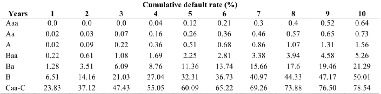
Figure 8 Average global cumulative historical default rates with respect to time Cumulative default rate (%)
Years 1 2 3 4 5 6 7 8 9 10 Aaa 0.0 0.0 0.0 0.04 0.12 0.21 0.3 0.4 0.52 0.64 Aa 0.02 0.03 0.07 0.16 0.26 0.36 0.46 0.57 0.65 0.73 A 0.02 0.09 0.22 0.36 0.51 0.68 0.86 1.07 1.31 1.56 Baa 0.22 0.61 1.08 1.69 2.25 2.81 3.38 3.94 4.58 5.26 Ba 1.28 3.51 6.09 8.76 11.36 13.74 15.66 17.6 19.46 21.29 B 6.51 14.16 21.03 27.04 32.31 36.73 40.97 44.33 47.17 50.01 Caa-C 23.83 37.12 47.43 55.05 60.09 65.22 69.26 73.88 76.50 78.54
Source: Moody’s Investor Service, April 2003
We can get the annual default probability from the previous table, through taking the difference in the cumulative default probability for each entry. Doing so, we get the following table:
Figure 9 Average global annual default rates with respect to time Default rate (%) Years 1 2 3 4 5 6 7 8 9 10 Aaa 0.0 0.0 0.0 0.04 0.08 0.09 0.09 0.10 0.12 0.12 Aa 0.02 0.01 0.04 0.09 0.10 0.10 0.10 0.11 0.08 0.08 A 0.02 0.07 0.13 0.14 0.15 0.17 0.18 0.21 0.24 0.25 Baa 0.22 0.39 0.47 0.61 0.56 0.56 0.57 0.56 0.64 0.68 Ba 1.28 2.23 2.58 2.67 2.60 2.38 1.92 1.94 1.86 1.83 B 6.51 7.65 6.87 6.01 5.27 4.42 4.24 3.36 2.84 2.84 Caa-C 23.83 13.29 10.31 7.62 5.04 5.13 4.04 4.62 2.62 2.04
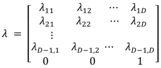
From the previous table we can see that the historical default probability stays constant or increases slightly in time for highly rated credit. However, for low credits such as Caa, the probability of a default decreases with increasing time. This seems quite intuitive, since for a company with a bad rating, the coming years are the most crucial ones. Once they have passed, it can be assumed that the probability of default declines. The last two tables only express the probability of a certain credit to move to default, i.e. to move to credit state, Jarrow, Lando and Turnbull use a transition matrix in their analysis. A transition matrix Λ shows the historical transition probability of a credit in state i to move to a credit in state j, within a certain time frame, thus
𝜆 = 𝜆!! 𝜆!" ⋯ 𝜆!! 𝜆!" 𝜆!! ⋯ 𝜆!! ⋮ 𝜆!!!,! 𝜆!!!,! ⋯ 𝜆!!!,! 0 0 1
Where the transition probabilities 𝜆!" ≥ 0 for all i,j. The probability of default for a certain credit state i, 𝜆!,! , is in the last column of Λ. The probability of survival for a bond in rating class i, 𝑄! = !!!𝑞!,! = 1 − 𝜆!,!. The probability of remaining in the same credit state is on the diagonal and is 𝜆!,! = 1 − !!!𝜆!,!
!!! .
The last row in Λ expresses that a credit that has defaulted stays in default. Hence, the transition probability 0, and the probability to stay in default is 1. In the following table, 82.83 reflects the probability of a credit, for instance a bond, which is currently rated A to stay in A; 0.47 reflects the probability of a bond that is currently rate A to migrate to B; 0.14 is the probability of a bond currently rated B to move to A.
Figure 10 One-year historical transition matrix of year 2002 (numbers in %) Rating at year-end
Aaa Aa A Baa Ba B Caa Default WR
Initial Rating Aaa 86.82 7.75 0 0 0 0 0 0 5.43 Aa 1.38 82.23 12.12 0.14 0 0 0 0 4.13 A 0 2.18 82.83 8.86 1.01 0.47 0.08 0.16 4.43 Baa 0.17 0.17 2.46 79.47 7.55 2.04 1.87 1.19 5.09 Ba 0 0.18 0.18 2.39 72.38 13.26 2.03 1.47 8.10 B 0 0 0.14 0.41 2.71 72.9 9.76 4.88 9.21 Caa 0 0 0 0 0.34 3.42 56.85 27.74 11.64
Source: Moody’s Investor Service, April 2003. WR represents companies that had been rated initially but are not rated at year-end
The next step is to transform historical default probabilities, derived from a transition matrix, into risk-neutral martingale probabilities in order to satisfy no-arbitrage conditions. This can be explained easier with an example.
Let’s assume we have four rating classes, A, B, C and default D. Let S01A, S01B, and S01C be the credit-spread, this is the difference between the yield of the risky bond and the yield of the risk-free bond, from time 0 to time 1 for a risky bond currently in rating class A, B, and C, respectively. Let’s assume S01A=0.01, S01B=0.015, and S01C=0.02, that can be rewrite in matrix form:
𝑆!"= 0.0150.01 0.02
.
Let S02A, S02B, and S02C be the credit-spread from time 0 to time 2 for a bond currently in rating A, B, and C, respectively. Let’s assume S02A=0.02, S02B=0.025, and S02C=0.03, hence:
𝑆!"= 0.0250.02 0.03
.
Let’s further assume the one-year historical transformation matrix:
𝑆 = 𝐴 𝐵 𝐶 𝐷 𝐴 0.70 0.15 0.10 0.05 𝐵 𝐶 𝐷 0.10 0.05 0.00 0.60 0.15 0.00 0.20 0.65 0.00 0.20 0.15 1.00
Though 0.7 is the probability of a bond currently rated A to stay in A; 0.2 is the probability of a bond currently rated B to be downgraded to C; 0.05 in the 2nd column and 4th row is the probability of a bond currently rated C to move to A. Let’s assume the risk-free continuously compounded interest rate from time 0 to time 1, r01 = 5% and the risk-free continuously compounded interest rate from time 0 to time 2, r02 = 6%. The recovery rate RR is assumed to be 40%.
In the risk-neutral environment, we can express the risky zero-coupon bond price B at time t with maturity T and notional of €1 as the value of the discounted expected future cash-flow of 1. We discount with the risk-free interest rate r plus the swap spread s:
𝐵!,! = 𝐸! 𝑒!(!!,!!!!,!)! (8)
where Et is the risk-neutral expectation value at time t, and s is the excess yield of the risky asset.
For a bond with a notional of € 1 that matures a time 1, the payoff at time 1 will be € 1 if the bond finishes in rating A, B, or C. The payoff will be the recovery rate RR, if the bond defaults. Including the historical default probabilities from the transition matrix, we can express the bond price B at time 0 with maturity 1, which is rated A, B01A as:
𝐵!"! = 𝑒!(!!,!!!!,!)! ≡ 𝑒!!!" 1 1 1 𝑅𝑅 𝐴 𝐴 𝐴 𝐴 𝐴 𝐵 𝐶 𝐷 (9)
where A → A is the historical probability of a bond in rating class A to stay in A; A → B is the historical probability of a bond currently in class A to move to B; and so on. Continuing with our example, we can state:
𝐵!"! = 𝑒! !.!"!!.!" ! ≠ 𝑒!!!" 1 1 1 0.4 0.70 0.15 0.10 0.05 or 𝑒! !.!"!!.!" ! = 0.9418 ≠ 𝑒!!.!" 1 1 1 0.4 0.70 0.15 0.10 0.05 = 𝑒!!.!" × 1×0.70 + 1×0.15 + 1×0.10 + 0.5×0.05 = 0.9227
As we can state, this result in an inequality, it is important to know that the equation (9) is not usually satisfied in reality.
Now, in order to satisfy the no-arbitrage condition (9), we have to transform the historical transition probabilities into risk-neutral martingale probabilities, which satisfy the condition (9).
In order to find the martingale probabilities λm, we have to adjust the historical probabilities λ with a factor η. η can be interpreted as a risk premium or risk adjustment. We can rewrite equation (9) for a bond currently rated in class A as:
𝐵!"! = 𝑒!(!!,!!!!,!)! ≡ 𝑒!!!" 1 1 1 𝑅𝑅 1 − (1 − 𝐴 → 𝐴 )𝜆! (𝐴 → 𝐵)𝜆! (𝐴 → 𝐶)𝜆! (𝐴 → 𝐷)𝜆! (10)
Generalizing the right side of the previous equation for a bond at time t with maturity T and solving for the risk adjustment of that bond in rating class i, ηi (we assume 𝑖 = 𝐴, 𝐵, 𝐶, 𝐷 ), we get:
𝜆! = 1 − !!!,! !(!!,!!!!,!)
! !
(!!!!)!!" (11)
One specific shortcoming of the model is that the default probability λi,D can become bigger than 1. This is especially the case for longer maturities T. Equation (11) can be reduced to:
𝜆!" = 1 − ! !!!,!!
!
(!!!!)!!. (12)
For this equation to be smaller than 1, we require that !
!!!,!! > 1 + 𝜆!(𝑅𝑅 − 1). This condition may not be satisfied for large s, T, η, and RR.
General shortcomings of the model lie again in the fact that the ultimate reason of default, the asset-liability structure or the liquidity of a company, is not part of the analysis. Also, as in the 1995 model, the interest rate process and the bankruptcy process are assumed independent. Furthermore, the recovery rate RR is exogenously given.
Naturally, the nature of the transition matrix also bears problems. Jarrow, Lando and Turnbull assume that bonds in the same credit class have the same yield spread. This is not necessarily the case as pointed out by (Longstaff & Schwartz, 1995). Rather, the rating-yield relationship is similar within sectors, which suggests conducting sector analysis, rather than aggregating data generally among counterparties.
An additional problem is that ratings are often done infrequently and may not be recent enough to reflect current counterparty risk. In addition, Standard & Poors currently only rates about 1% of all companies worldwide. Nevertheless, the number of rated companies should increase in the future, allowing a widespread usage of the model and its extensions.
Duffie and Singleton (1999)
(Duffie & Singleton, 1999) express the risky bond price B at time t with maturity T based on equation 𝐵!,! = 𝐸! 𝑒!(!!,!!!!,!)! . In the Duffie-Singleton model, the swap spread St,T equals approximately 𝜆!(1 − 𝑅𝑅). This result can be derived by a simple binomial tree for a zero-coupon bond with maturity at time 1 and a notional amount of € 1, as shown in the next figure:
Figure 11 Deriving the swap spread s
In the last figure, r is the risk-free interest rate, s is the swap spread, λ is the hazard
rate, which multiplied by time periods for default of 1 equals the risk-neutral probability
of default. RR is the recovery rate. Then, we can derive:
𝑒!(!!!) = 𝜆𝑒!!𝑅𝑅 + (1 − 𝜆)𝑒!!. (13)
Solving the last equation for s, using 𝑒! ≈ 1 + 𝑥, we get 𝑠 ≈ 𝜆 1 − 𝑅𝑅 + 𝜆𝑟 1 − 𝑅𝑅 . Duffie and Singleton prove than the term 𝜆𝑟 1 − 𝑅𝑅 can be dropped for a continuous time setting. Hence, the interest rate process drops out and we can write for a default swap spread from time t to time T, St,T:
𝑆!,! ≈ 𝜆!,!(1 − 𝑅𝑅) (14)
Where all variable are viewed at time t.
The last equation shows the intuitive approximate relationship between the swap spread
s and a hazard rate λ. If the recovery rate RR is zero, 𝑠!,! ≈ 𝜆!,!. Hence the spread s approximately compensates the investor for the default risk λ. The relationship in the equation 𝑆!,! ≈ 𝜆!,!(1 − 𝑅𝑅) is often termed credit triangle, since two of the three variables are sufficient to generate the third.
The model may include a liquidity premium l for the risky asset. In this case the swap spread is simply:
𝑆!,! ≈ 𝜆!,!(1 − 𝑅𝑅) + l (15)
where l is a fractional value of the risky bond.
Duffie and Singleton show that any risky claim B with an notional amount N, for different interest rates r and swap spreads s at various times j, and time units of 1, with maturity t + τ, can be expressed as:
𝐵!,!!! = 𝐸! 𝑒! !!!!!!(!!!!!!!!!)𝑁
!!! (16)
Hence, one crucial finding of the Duffie-Singleton model is that any risky claim B can be priced by discounting the notional amount N with the default-adjusted process r+s.
𝑒!(!!!)
𝑅𝑅 λe-r
1 (1- λ)e-r
The equation 𝐵!,!!! = 𝐸! 𝑒! !!!!!!(!!!!!!!!!)𝑁
!!! is an extension of the equation 𝐵!,! = 𝐸! 𝑒!(!!,!!!!,!)! .
In the last equations, the recovery rate RR is applied to the expected market value of the risky bond at the time of default, termed recovery of market value RMV, hence 𝐸! 𝑅𝑀𝑉!!! = 𝑅𝑅!𝐸! 𝐵!!! , where d+1 is the time of default. In contrast, in the Jarrow-Turnbull 1995 and Jarrow-Lando-Turnbull 1997 model, the recovery value is a fraction of the risk-free bond price at the time of default. Brennan-Schwartz (1980), Longstaff-Schwartz (1995), and Duffie (1998) apply a simpler assumption with respect to the payoff in default. They assume that creditors at the time of default receive the recovery rate multiplied with the notional amount of the risky bond.
O’Kane and Turnbull (2003)
(O' Kane & Turnbull, 2003) presents in their paper a market standard pricing model. Their approach is based on the work of Jarrow and Turnbull (1995), who characterized a credit event as the first event of a Poisson counting process which occurs at some time τ with a probability defined as:
𝑃𝑟 𝜏 < 𝑡 + 𝑑𝑡|𝜏 ≥ 𝑡 = 𝜆 𝑡 𝑑𝑡 (17)
ie, the probability of a default occurring within the time interval 𝑡, 𝑡 + 𝑑𝑡 conditional on surviving to time t, is proportional to sometime dependent function λ(t), known as the hazard rate, and the length of the time interval dt. We can therefore think of modelling default in a one-period setting as a simple binomial tree in which we survive with probability 1-λ(t)dt, or default and receive a recovery value R with probability λ(t)dt. O’ Kane and Turnbull make the simplifying assumption that the hazard rate process is deterministic. By extension, their assumption also implies that the hazard rate is independent of interest rates and recovery rates.
Figure 12 The equivalent of a binomial tree in the modelling of default in which the tree terminates and makes a payment K at default
Extending this model to continuous time survival probability to time T conditional on surviving to valuation time, 𝑡!, by considering the limit dsè0.
Survival probability can be shown as
𝑄 𝑡!, 𝑇 = exp − !!𝜆 𝑠 𝑑𝑠
! . (18)
This model is used to value both the premium and protection legs, and then the breakeven spread of a default swap. With this model, we can get the implied term structure of arbitrage-free survival probabilities from market spreads.
In order to value the premium leg, this is the series of payments of the default swap spread made to maturity or to the time of the credit event, which occurs first, and ignoring the accrued premium payment from the previous premium payment date until the time of the credit event, the present value of the premium leg can be written as:
𝑃𝑟𝑒𝑚𝑖𝑢𝑚 𝐿𝑒𝑔 𝑃𝑉 𝑡!, 𝑡! = 𝑆 𝑡!, 𝑡! ! Δ
!!! 𝑡!!!, 𝑡!, 𝐵 𝑍 𝑡!, 𝑡! 𝑄 𝑡!, 𝑡! . (19) where there are n=1,…,N contractual payment dates t1,…,tN and tN is the maturity date of the default swap, with the spread 𝑆 𝑡!, 𝑡! between today and the maturity date. ∆ 𝑡!!!, 𝑡!, 𝐵 is the day count fraction between premium dates tn-1 and tn in the appropriate basis convention denoted by B. 𝑄 𝑡!, 𝑡! is the arbitrage-free survival probability of the reference entity from the valuation time tv to premium payment time
tn. 𝑍 𝑡!, 𝑡! is the Libor discount factor from valuation date to premium payment date n.
In order to include the effect of premium accrued, we have to work out the expected accrued premium payment by considering the probability of defaulting at each time
R R R R R λ(s)ds λ(s+ds) λ(s+2ds)ds λ(s+(N-1)ds)ds 1-λ(s+(N-1)ds)ds 1-λ(s+2ds)ds 1-λ(s+ds)ds 1-λ(s)ds
between two premium dates, and calculating the probability weighted accrued premium payment, resulting in the following expression for the premium leg:
𝑆 𝑡!, 𝑡! !!!! !!!!!! Δ 𝑡!!!, 𝑠, 𝐵 𝑍 𝑡!, 𝑠 𝑄 𝑡!, 𝑠 𝜆 𝑠 𝑑𝑠. (20) This integral makes complicated expression to evaluate exactly. Though, as demonstrated by O’ Kane and Turnbull, it is possible to approximate this equation with
! !!,!!
! !!!!Δ 𝑡!!!, 𝑡!, 𝐵 𝑍 𝑡!, 𝑡! 𝑄 𝑡!, 𝑡!!! − 𝑄 𝑡!, 𝑡! (21) by noting that if a default does occur between two premium dates, the average accrued premium is half the full premium due to be paid at the end of the premium period. The full value of the premium leg is then given by
𝑆 𝑡!, 𝑡! ×𝑅𝑃𝑉01 (22)
where RPV01 is the risky PV01 defined as
𝑅𝑃𝑉01 = ! Δ
!!! 𝑡!!!, 𝑡!, 𝐵 𝑍 𝑡!, 𝑡! 𝑄 𝑡!, 𝑡! +!!"! 𝑄 𝑡!, 𝑡!!! − 𝑄 𝑡!, 𝑡! (23) where 1PA=1 if the contract specifies premium accrued (PA) and 0 otherwise.
The effect of premium accrued on the spread can be very well approximated by 𝑆!
2 1 − 𝑅 𝑓
The protection leg is the contingent payment of (100%-R) on the face value of the protection made following the credit event. R is the expected recovery rate. In pricing the protection leg, it is important to take into account the timing of the credit event, because this can have a significant effect on the present value of the protection leg – especially for longer maturity default swaps. Within the hazard rate approach we can solve this timing problem by conditioning on each small time interval 𝑠, 𝑠 + 𝑑𝑠 between time tv and tN at which the credit event can occur. The expected present value of the recovery payment is:
(1 − 𝑅) !!𝑍 𝑡!, 𝑠 𝑄 𝑡!, 𝑠 𝜆 𝑠 𝑑𝑠
!! (24)
where, R is the expected recovery price of the cheapest to deliver asset at the time of the credit event, 𝑄 𝑡!, 𝑠 is the probability of surviving to some future time s. 𝑍 𝑡!, 𝑠 is the risk free rate between today and the future time s, and 𝜆 𝑠 𝑑𝑠 is the probability of a credit event in the next small time increment ds.
From now on, it is possible to get the survival probabilities from the market quoted default swap spread, through
Other significant reduced form models that have received recognition are Brennan-Schwartz (1980); Iben-Litterman (1991); Longstaff-Brennan-Schwartz (1995); Das-Tufano (1996); Duffee (1996); Schoenbucher (1997); Henn (1997); Brooks-Yan (1998); Madan-Unal (1998); Duffee (1998); Das-Sundaram (2000); Hull and White (2000); Hull and White (2001); Wei (2001); Duffie-Lando (2001); and Jarrow-Yildirim (2002); Martin, Thompson and Browne (2003)
Analysis Framework
Credit Default Swaps in numbers
In 1998, International Swaps and Derivatives Association (ISDA®) facilitated the CDS trading, through standard documentation and procedures, allowing credit risks to be traded and managed in much the same way as market risks. In 2009, the market saw a “Big Bang” for CDS contracts and the way in which they are traded, including important convention changes in order to make CDS more standardised to help support efforts for central clearing of CDS trades.
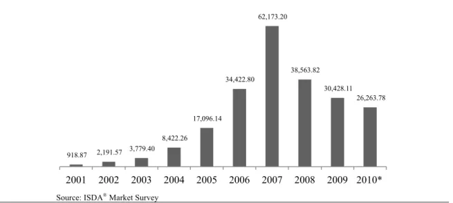
According to the ISDA® market survey, the notional amount outstanding of CDS had an outstanding expansion in the last decade, rising from US$920 billion at 2001 to US$62.2 trillion at 2007. This breakthrough growth was interrupted by a financial turmoil starting in 2007, caused by a subprime mortgage crisis, and then by the Lehman and Brothers, AIG and Bern and Stearns bankruptcy, downing to US$26.3 trillion at mid-year 2010, a decrease of 57.8% from year-end 2007.
As in past surveys held by ISDA®, the US$26.3 trillion notional amount was approximately evenly divided between bought and sold protection: bought protection notional amount was approximately US$13.3 trillion and sold protection was about US$13.0 trillion, with a net bought notional amount of US$359.0 billion, representing 5.6% of the total derivatives reported to the ISDA® Market Survey.
Figure 13 Outstanding Credit Default Swaps. Notional amounts in billions of US dollars, adjusted for double counting
Source: ISDA® Market Survey
According to ISDA® CDS Marketplace™, in May 5th 2012 the total par amount of credit protection bought or sold was around US$14.9 trillion, 81% was related to
918.87 2,191.57 3,779.40 8,422.26 17,096.14 34,422.80 62,173.20 38,563.82 30,428.11 26,263.78 2001 2002 2003 2004 2005 2006 2007 2008 2009 2010*
corporates and the rest to sovereigns. More than 91% of this amount, mentioned as gross notional value in ISDA® studies was concentrated in Europe and America.
It is important to refer the overall amount of credit risk in the financial system does not increase with this significant size of the credit derivatives market, because every credit derivative contract has a buyer and a seller of the credit risk and so there is no net increase of credit risk. In some situations credit derivatives can increase the amount of credit risk in the capital markets, due to the counterparty credit risk associated with each contract. This is the risk that the protection seller does not pay the compensation in case of default to the protection buyer.
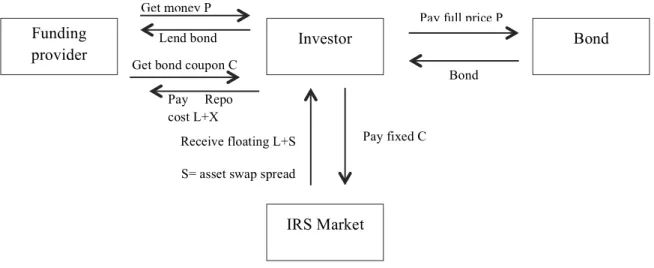
The equivalence relation between CDS and bond yields
In our study, we will use the reduced-form hence it offers a suitable framework to connect bond spreads with CDS premia. Using the risk neutral default probability and no-arbitrage conditions, it is direct to establish the parity link between the two spreads, which will be used as the testable hypothesis in the empirical part of the thesis.
This framework, initially developed by (Duffie, Credit swap valuation, 1999), is simplified by assuming that the risk-free rate (r) is constant over time. The protection buyer of a CDS must pay a constant premium (s) until the contract matures or a credit event occurs to the protection seller. If a credit event does occur, the protection buyer receives the difference between the cheapest-do-deliver bond and the face value, and must pay accrued CDS premium upon default. For simplicity, we will assume the recovery value as the difference between the par value and the market value and there is no accrued premium after default.
Assuming no-arbitrage conditions, we can replicate synthetically the acquisition of a CDS through shorting a par fixed coupon bond, with a coupon rate of (c) on the same reference entity with the same maturity date, and investing the proceeds in a par fixed coupon risk-free bond. Therefore, the CDS premium should be equal to the credit spread of the par fixed coupon bond. That is,
s = c – r (25)
If this parity relationship is violated, the arbitrageur can take profits. This is, if s > c – r, an investor can sell the CDS in the derivatives market, buy a risk-free bond and sell the bond of the reference company in the cash market, resulting in arbitrage returns.
If s < c – r, the investor can implement the reverse strategy in order to collect profits. Meanwhile, this equilibrium may not hold, because some of the key assumptions may not be satisfied in practice. First, the protection buyer normally needs to pay the accrued premium when the credit event occurs, making the CDS premium to be smaller after taking into the account of this accrued payment. Second, the existence of the cheapest-to-deliver option, hence the majority of the CDS contracts are settle via physical delivery, resulting in an increase of the CDS premia. Third, the definition of credit
event is not unanimous, making harder the valuation of a credit event. Fourth, there is no initial exchange of cash-flows in a CDS transaction, in contrast to the bond market. This difference could cause the CDS market to respond faster than the bond market to changes in the underlying credit risk, generating price discrepancies in the short run. Fifth, short-sale of corporate bonds is practically not allowed, making difficult to gain from the price difference when the CDS premium is higher than the bond spread. This asymmetry may have important implications for the credit spreads adjustment dynamics. Sixth, transaction costs will reduce the number of arbitrage opportunities between the two markets. Lastly, the two spreads may be influenced differently by other factors than credit risk, such as liquidity and/or counterparty risk.
Consequently, in our study we will assume that:
1. Market participants can short single name corporate bonds. This means that bond holders can sell bonds, buy riskless bonds and sell default protection when
s > c – r;
2. Market participants can short riskless bonds. This is equivalent to assuming that market participants can borrow at the risk free rate;
3. We ignore the cheapest-to-deliver bond option in a CDS; 4. There is no counterparty default risk in a CDS;
5. The circumstances under which the CDS pays off are those defined by ISDA®; 6. We ignore that there may be tax and liquidity reasons that cause investors to
prefer a riskless bond to a corporate bond plus a CDS or vice versa; 7. CDS gives the holder the right to sell a bond for its face value; 8. We ignore transaction costs.
Estimation of risk-neutral default probabilities from CDS spreads
As we state previously, we will use the reduced form to modelling credit events and estimate our risk-neutral default probabilities from CDS spreads through optimization algorithm, based on the work of (Martin, Thompson, & Browne, 2001). Thus, we will assume the default process to follow an non-homogeneous Poisson process and as such for any 0 ≤ τ ≤ T the default time t and default intensity λ(t) satisfy
𝑄! 𝑡 = ℙ 𝜏 > 𝑡 = 𝑒𝑥𝑝 − !!𝜆 𝑢 d𝑢 (26)
where ℙ is the risk-neutral probability and T is the final maturity. The single name survival probabilities ℙ (τ > t ) are usually implied from the CDS market.
The fair CDS spread balances the present value of the contingent leg C, given by 𝐶 = 𝑁(1 − 𝑅) ! 𝑑(𝑡!)(𝑄! 𝑡!!! − 𝑄! 𝑡! )
!!! (27)