FACULDADE DE ENGENHARIA DA UNIVERSIDADE DO PORTO
MASTER THESIS
DEVELOPMENT OF A LOW FIDELITY PROCESS
MODEL FOR ADDITIVE MANUFACTURING.
Computational Mechanics master
Author:
MANUEL JIMÉNEZ ABARCA
Supervisors:
OLE SIGMUND, ANDERS CLAUSEN, CESAR DE SÁ
2
Acknowledgment.
This Master Thesis was carried out at the Institute of Science and Innovation in Mechanical and
Industrial Engineering (INEGI1) in Porto and at Technical University of Denmark (DTU) in Lyngby
between January and September 2020 as a part of the Computational Mechanics program from the Faculty of Engineering at University of Porto (FEUP).
I would like to thank my supervisor at DTU Dr. Ole Sigmund for guiding the decisions made and his support during the complete work here presented. I would also like to thank the members from the Oqton company Anders Clausen and Erik Andreassen for providing the data related to the experimental print and their advice about the printing outcomes. Also, a kindly thanks to my supervisor at FEUP Dr. José Cesar de Sá for tracking my progress and giving me the opportunity to start researching at INEGI in the additive manufacturing field. A friendly thanks to my colleague at INEGI Roya Darabi for the positive co-working experience. Finally, a warm thanks to my parents Manuel Jimenez and Maria Angeles Abarca for supporting me from the beginning of my studies.
Sincerely,
Manuel Jimenez Abarca
1 through funding of Project ADDing (POCI-01-0145-FEDER-030490), co-financed by Fundo Europeu de Desenvolvimento Regional (FEDER) through Programa Operacional Competitividade e
3
Abstract.
Additive manufacturing of metal components is a complex process that involves an exhaustive experimental work to achieve the demands of the customers. The computer simulation is a powerful tool to support the experimental work and reduce the lead time and cost required. However, the simulation process has its own challenges.
The finite element-based software Abaqus is selected to run two different methods of printing simulation: thermo-mechanical and Inherent strains-based. The presented models are classified according to the level of fidelity of the solution. Two studies are carried out: comparison of the thermo-mechanical models in a scaled part and validation of the simulation methods in an industrial-size part. Data from experimental prints is used to validate the results of the simulations. The trade-off between accuracy and computational cost is examined. In addition, the capabilities of the software to implement the complete manufacturing process are evaluated.
A deep knowledge of the manufacturing process and the finite element software is required to successfully simulate the final state of a printed component. The Inherent strains-based method is a better choice in terms of efficiency and accuracy than the thermo-mechanical method to model parts typically printed in the additive manufacturing industry. The software allows to simulate the whole metal printing process but presents some limitations in the implementation.
Keywords: Additive manufacturing, selective laser melting, finite elements method, Inherent
5
Index
1. Introduction. ... 12
1.1. Motivation. ... 12
1.2. Additive Manufacturing. ... 12
2. Finite Elements Analysis. ... 16
2.1. Thermo-mechanical simulation. ... 16
2.1.1. Progressive element activation. ... 17
2.1.2. Moving heat source. ... 18
2.1.3. Thermal losses. ... 21
2.2. Inherent strains-based simulation. ... 21
2.2.1. Progressive element activation. ... 22
2.2.2. Pattern-mesh intersection. ... 23
3. Basis formulation and governing equations. ... 26
3.1. A non-linear finite element approach. ... 26
3.2. Thermal model ... 26 3.2.1. Thermal equilibrium. ... 27 3.2.2. Boundary conditions. ... 27 3.3. Continuums mechanics. ... 28 3.3.1. Elasticity. ... 28 3.3.2. Boundary conditions. ... 29 3.3.3. Plasticity. ... 29 3.3.4. Inherent strains. ... 31 4. Material modelling. ... 32 4.1. Material selection. ... 32
4.2. Latent heat effect... 34
4.3. Plasticity model. ... 35
5. Geometry selection. ... 37
6. Scaled model... 39
6.1. Part-fixing. ... 39
6.2. Tool path and scanning strategy. ... 40
6.3. Level of fidelity. ... 41 6.4. Boundary conditions. ... 42 6.5. Interactions. ... 43 6.6. Printing parameters. ... 44 6.7. Cooling. ... 45 6.8. Mesh. ... 45 6.9. Time-stepping ... 46 6.10. Results. ... 47 6.10.1. Thermal results. ... 47
6
6.10.1.2. Medium Fidelity model. ... 50
6.10.2. Mechanical results. ... 51
6.10.2.1. High Fidelity model. ... 51
6.10.2.2. Medium Fidelity model. ... 53
6.10.3. Models comparison. ... 54
6.10.4. Computational cost. ... 56
7. Real model. ... 57
7.1. Part-fixing. ... 57
7.2. Inherent strains application. ... 59
7.3. Boundary conditions. ... 61 7.4. Interactions. ... 61 7.5. Printing parameters. ... 62 7.6. Mesh. ... 63 7.7. Time-stepping ... 64 7.8. Results. ... 65 7.8.1. After printing. ... 65 7.8.2. Supports removal. ... 68 7.8.3. Heat treatment. ... 70 7.9. Experimental data. ... 74 7.9.1. Available data. ... 74 7.9.2. Measurement methodology. ... 74 7.9.3. Results. ... 76 7.10. Results comparison. ... 77
7.10.1. Non-heat treated part. ... 77
7.10.1.1. Low Fidelity model. ... 78
7.10.1.2. Medium Fidelity model. ... 80
7.10.2. Heat treated part. ... 82
7.11. Computational cost. ... 83
8. Conclusions. ... 84
9. Assessment of the work done. ... 86
9.1. Objectives achieved. ... 86
9.2. Limitations and Future work. ... 86
A. Appendix. ... 89
A.1. Collaborating organizations. ... 89
A.2. Convergence studies. ... 89
A.2.1. Mesh convergence. ... 89
A.2.2. Time increment convergence. ... 95
7
.List of Figures
1 SLM manufacturing process . . . 14
2 Removable Partial Denture (RPD) stent fabricated using SLM technology. . . 14
3 Cranial prothesis made by an AM metal process. . . 14
4 Point, infinite line and box toolpaths. . . 18
5 Infinite line toolpath-mesh intersection. . . 18
6 Point toolpath-mesh intersection. . . 20
7 Box toolpath-mesh intersection . . . . . . . 20
8 Goldak volume-based energy distribution. . . 20
9 Simulation steps required in the IS method. . . 23
10 Example of Island pattern strategy for IS method. . . 24
11 Scan pattern – element intersection [11]. . . 24
12 Visualization of the first component of the inherent strains in a simple cube. . . 25
13 Stresses and strains in the HAZ during SLM process. . . . 30
14 Ti6AlV4 thermal properties evolution. . . 33
15 Ti6AlV4 mechanical properties evolution. . . 33
16 Ti6AlV4 thermal expansion coefficient. . . 34
17 Latent heat effect in a metal material. . . 35
18 Hardening model with annealing temperature effect . . . 36
19 Front and top views (left) and isometric view (right) of the Real part. . . . 37
20 Front and top views (left) and isometric view (right) of the Scaled part. . . . . 38
21 Build plate top and front view. . . .39
22 Scanning strategy of the Scaled model.. . . 41
23 Contact surface between build plate and part. . . . . 43
24 8 nodes linear brick element.. . . .46
25 Mesh distribution for the part (left) and the build plate (right).. . . .46
26 Isosurface of the melting pool gradient for the High-fidelity model. . . . 48
27 Cross section and depth views of the molten pool for the High-fidelity model.. . 49
28 Thermal history of the node 971 for the High-fidelity model.. . . . 49
29 Thermal history of the node 4759 for the MF scaled model. . . . .50
30 Node evaluated (red point) for the MF scaled thermal history. . . .51
31 Distortions in X-direction U1 (left), Y-direction U2 (centre) and Z-direction U3 (right) for the HF model. Units in mm. . . . . . . 52
32 Temperature field comparation between left side (top) and right side (bottom) of the HF model. Toolpath depicted in red on the right. . . . . 52
33 Von Mises stress σVM (MPa) for the HF model. . . . . 53
34 Displacement magnitude U in mm for the MF model. . . . . .54
35 Von Mises stress σVM distribution (left) and stress singularity (right) for the MF model. . . . . . . . 54
36 Locations evaluated for the models’ comparison of UX (blue) and UY (red). . . . . . . . 55
37 Cross-sections at z = 4 mm of the MF model (red) and HF model (blue) after print. Measurements in mm. . . . 56
38 Support’s geometry (left) and distribution along the part (right). Dimensions in mm. . . . 58
39 Build plate top and front view. Dimension in mm. . . . 59
40
𝜀
11∗ state before the addition of a new element layer (left) and after the addition of a new element layer (right). . . . . . . . 608
42 Scanning strategy of the Real model . . . . . . . . . . . . 63
43 Mesh distribution for the supports and part (left) and the build plate (right). . . . 64
44 Distortions in X-direction U1 (left), Y-direction U2 (centre) and Z-direction U3 (right) for the LF model. Units in mm. . . . . . 66
45 Distortions in X-direction U1 (left), Y-direction U2 (centre) and Z-direction U3 (right) for the MF real model. Units in mm. . . 66
46 Detail of the distortions in Z-direction U3 for the MF model. . . . 67
47 Cross-sections at z=20 mm of the LF model (red) and MF model (blue) after print. Measurements in mm. . . . 67
48 Stress distribution in MPa in the outer face (left) and a detail in the support’s area (right) for the LF model. . . . 68
49 Stress distribution in MPa in the outer face (left) and a detail in the support’s area (right) for the MF real model. . . . 68
50 Section of the supports cut from the LF model. . . .69
51 Locations constrained in X-direction (top), Y-direction (bottom left) and Z-direction (bottom right) for the cutting procedure. . . . . 69
52 Stress distribution before cut (left) and after cut (right). . . 70
53 Comparison of cross-sections of the part before cutting (dark blue) and after cutting (light blue). . . . . 70
54 Annealing heat cycle . . . 72
55 Stress-temperature annealing cycle on LF model. Stress (blue), temperature (red). . . . . 72
56 Point evaluated during the Annealing treatment (highlighted in red). . . . . 73
57 Stress – creep strain relationship during the annealing treatment. Stress (blue), strain (orange). . . . 73
58 Bottom cross-sections of the LF model with annealing treatment (red) and without annealing treatment (blue). . . . 74
59 Inspection machine developed by Oqton® to scan the experimental parts. . . 75
60 Scanned part before removal of the clamp (left) and after removal of the clamp (right). . . . 75
61 Measurements in the experimental parts. . . 76
62 Contour shape comparison between the original part (blue) and experimental Part1 (red) for the Non-HT case. . . 77
63 Error in the application of the Inherent strains on the last element layer . . . 78
64 Deformed shape of the Part1 (red) and the LF part (blue) for the non-heated treatment case. . . . 79
65 Cross-section’s contour at z=12 mm of the experimental part (red) and LF model (blue). Measurements in mm . . . 79
66 Residual stress presented in MF model after printing. Von Mises stress in MPa. . 80
67 Closing effect. Deformed shape after printing (blue) and after stresses release (red) for the MF model. . . . . 81
68 Support’s top surface deformation after printing for the MF model. Displacements in mm. . . . 81
9
List of Tables.
1 Material basic properties. . . 33
2 Laser scanning parameters of the Scaled model. . . . 40
3 Laser energy distribution parameters. . . . 44
4 Laser scanning parameters of the Real model. . . . 63
5 Creep law parameters. . . 72
6 Measurements of the experimental parts after cut for the HT and Non-HT parts . 76 7 Experimental - simulated model comparison for the Non-HT case. . . 77
10
Notation.
Symbol Unit Description
q mW/mm2 Heat flux density
x, y, z mm Cartesian coordinates
Q mW Input energy
η - Absorption coefficient
P mW Laser power
r mm Laser spot radius
e - Laser spot eccentricity
d mm Laser spot depth
φ - Patch local angle
ϴ - Interlayer rotation angle
U - Solution vector
R - Residual vector
Δt s Time step
Cp mJ/(t∙K) Specific heat capacity
Θ K Temperature
t s Time
𝑟⃗ mm Relative spatial coordinate
k mW/ (mm∙K) Thermal conductivity
qk mW/mm Heat flux conduction
h mW/ (mm2∙K) Film coefficient
σ mW/ (mm2∙K4) Stefan-Boltzmann constant
𝜖 - Emissivity
𝜎⃗ MPa Tension vector
𝜀⃗ - Deformation vector
E MPa Young modulus
ν - Poisson’s coefficient
σy MPa Yielding stress
u mm Displacement
α 1/K Expansion coefficient
𝜀̇ - Strain rate
σVM MPa Von Mises stress
11
Acronyms.
Abbreviation Meaning
AM Additive Manufacturing
CAD Computer Aided Design
DED Direct Energy Deposition
PBF Powder Bed Fusion
EBM Electron Beam Melting
SLM Selective Laser Melting
CNC Computer Numerical Control
FEM Finite Element Method
CAE Computer Aided Engineering
HAZ Heat Affected Zone
TGE Temperature Gradient Effect
STL STereoLithography
BC Boundary Conditions
NIST National Institute of Standards and Technology
HF High Fidelity
MF Medium Fidelity
LF Low Fidelity
12
1. Introduction.
1.1.
Motivation.
The simulation of additive manufacturing (AM) processes has traditionally demanded a high computational cost translated into powerful computers and large running times. It derives from the refined solution needed to capture the large temperature gradients in very short times presented in the building process. These simulations generate very accurate results and the models are called “High fidelity” models. However, an approximate model can often be
sufficient to guide manufacturing choices.
The objective of this work is to create a “Low fidelity” model which approximates the final state of the printed part at a substantially lower computational cost. For that purpose, an inherent strain-based calculation method is used together with other simplifications. The trade-off between accuracy and computational cost is examined and the results compared with higher fidelity and experimental ones.
As a result, the approximate model is validated, and the modelling choices made in this work can be useful to guide future AM modelling under similar conditions.
1.2.
Additive Manufacturing.
AM or, commonly referred as 3D printing, describes the modern technology which automatically builds up parts layer by layer using a Computer Aided Design (CAD) file. Parts can be produced in complex forms that are not possible to be produced using traditional manufacturing methods. In addition, it does not rely on expensive tooling having essentially no start-up costs. That also leads to rapid verification and development of prototypes and low-volume production parts. However, this technology presents some limitations. The main one is the inability to produce parts with material properties equivalent to those made via subtractive or formative procedures [1]. Basically, the parts produced are inherently anisotropic and not fully dense. AM also has limitations in repeatability due to variations during cooling.
The different AM technologies can be classified according to the material used: polymer or metal. Metal 3D printing allows to produce high-quality, functional and load bearing parts. They can also be divided by the way the material is placed on the build plate in depositing or powder bed processes [1]. The deposition process is made by the printing nozzle at the same
13
time as the material is heated. An example is the Direct Energy Deposition (DED) process, typically used to repair or add additional material to existing components. On the other hand, in the powder bed fusion (PBF) processes the material is spread over the building plate and, subsequently, melted by the energy source. Lastly, PBF processes can be differentiated according to the energy heat source in Electron Beam Melting (EBM) and Selective Laser Melting (SLM).
The PBF process has 4 steps depicted in figure 1:
• 1. A thin layer of the powder material is spread along the build plate surface. • 2. The high-powered laser scans a single cross section of the part and fuse it
with the material underneath.
• 3. An elevator lowers the build plate by the thickness of the powder layer. • 4. A roller pushes a new layer of powder over the built component. The steps 2,
3 and 4 are repeated until the part is completed.
The main limitations of SLM are cost and build size. Thus, only the critical and complex parts of a design should be printed. The simpler sections should be machined by Computer Numerical Control (CNC) and then assembled.
SLM suits better in dental, medical, aerospace and automotive applications where the fundamental benefits of AM are required [1]. SLM has become popular in the dental industry to produce crowns, bridges and stents like the ones shown in figure 2. The possibility of producing a large number of customised parts in a single print has significantly accelerated the manufacturing process. The medical industry has also embraced AM. The high level of freedom in the design enables an exact fit in the patient’s anatomy and can include unique surface characteristics (like porosity) to imitate biological textures. Figure 3 shows an example of a customized cranial prothesis. Related to the aerospace and automotive industries the SLM process plays an important role in parts where weight reduction is a critical design parameter. SLM also ensures the production of complex parts with a high strength and made of high-performance metals.
14
Figure 1: SLM manufacturing process [2].
Figure 2: Removable Partial Denture (RPD) stent manufactured using SLM technology.
15
The aforementioned benefits of AM and specially of the SLM process have created an excitement atmosphere about this technology. However, the process is not as simple and accurate as promised. The involving change of phase (melting and solidification) of a material region over a much cooler body produces expansion and contraction in the part which leads to permanent warping as well as to high residual stresses [4]. Residual stresses can cause failure during printing or during the in-service life of a part. The distortion imperils the economic feasibility of producing parts using the AM technology as, usually, iterative builds are required to minimize the warping. Each experimental test can take hours to days to complete with the consequent cost. Thus, modelling of the thermo-mechanical behaviour becomes a complement or even an alternative to repetitive experimental tests. The objectives of the AM simulation are to [5]:
• Predict the residual stresses in a part.
• Minimise the gap between the designed and manufactured part through process optimization.
• Evaluate how a manufactured part performs under realistic loading conditions in an assembly with other components.
Modelling an AM process has its own challenges. First, implementing the progressive material addition and then to deal with the non-linearities introduced by the thermal dependence of the material properties as well as the material state change. Related to the mechanical behaviour, a proper plasticity model must be implemented. In addition, due to the transient characteristic of the process, the discretization both in space and time may require expensive computational resources and a deeper understanding of computational methods to achieve accurate results in a feasible time.
16
2. Finite Elements Analysis.
The Finite Element Method (FEM) has been consolidated over the last decades as the main solution for Computer Aided Engineering (CAE) problems. The novel AM technology is not an exception and numerous FEM commercial software packages have implemented the mechanisms needed to accurately simulate the process. The modelling of the SLM process must overcome the following challenges:
• Progressive Material addition. • Moving heat source input. • Thermal losses during building. • Thermo-mechanical coupling.
• Material properties dependence on temperature.
From the different software available Abaqus/Standard from Dassaults Systèmes® is selected due to its special AM plug-in. The plug-in consists of pre-defined tables and modules that allows to model in a detailed and efficient way. Abaqus does not only implement a solution for the aforementioned challenges, but it is developed in a user subroutine structure and keywords interface that provides a high degree of control and customization. Abaqus/Standard
uses thermo-mechanical and eigenstrain analyses for the simulation of AM processes.
2.1.
Thermo-mechanical simulation.
A thermal-stress analysis allows exact specification in time and space of processing conditions and control over the fidelity of the solution. It is usually more accurate but more computationally expensive than the pure mechanical eigenstrain analysis.
The thermal-stress analysis is decoupled or weakly coupled, assuming that the thermal behaviour affects the mechanical one, but the mechanical response does not affect the thermal history. This is due to the fact that the energy from the heat source is very large compared to the strain energy stored in the workpiece [6]. The process turns into a sequential simulation where the heat transfer problem is solved first and then the mechanical response. Basically, the thermal loads introduced by the printing process results in a temperature field which drives the static structural analysis.
17
2.1.1. Progressive element activation.
The layer by layer deposition of raw material from a roller and the melting process are modelled using progressive element activation. The elements with the activation feature on can be activated by assigning a volume fraction of material at the beginning of the increment. Both full and partial activation are implemented. The addition of material into a numerical model means the addition of new equations. To account for this, the “Dead-alive” method is used which adds the new equations into the matrices over the history of the model [7].
The elements get activated when they are intersected by a tool path. Abaqus presents the Toolpath-mesh intersection module to compute the geometric intersection between several toolpaths and the finite element mesh of the part to be manufactured. A toolpath is defined by a geometric shape attached to a reference point that moves along a path. The path is defined by connecting a collection of points in space and time. An event series defines the collection of points [8]. The three shapes considered for toolpath-mesh intersection are illustrated at the figure 4.
For example, the infinite line representation is useful to describe the process of layer-by-layer material deposition, such as the activation of the roller in PBF [9]. Figure 5 depicts the intersections of an infinite line toolpath with a finite element, E. The toolpath is defined by an
infinite line attached to a reference point that is moving along the path connecting points (X1,
X1, X1, … XN) such that the reference point is at Xi at time 𝑡i . For a given element, the
toolpath-mesh intersection module computes the number of intersections, m, and the volume fraction,
vf, for each intersection. The volume fraction is equal to the ratio of the partial volume of the
element below the z-plane defined by the motion of the infinite line following the path to the
total volume of the element. The module also computes the area A; the coordinate Xa with
respect the element reference coordinate system of the centre of the intersection of the z-plane and the element; as well as the area fractions, 𝑎𝑖𝑓, below the z-plane for all sides for each intersection [8].
18
Figure 4: Point, infinite line and box tool shapes [8].
Figure 5: Infinite line toolpath-mesh intersection [8].
2.1.2. Moving heat source.
The recently deposited layer of material gets heated up to the melting point, causing the material to fuse to the solid material underneath. For that purpose, the modelling of the heat source is required. The challenges are to accurately capture the size and shape of the energy distribution and to estimate the amount of heat actually absorbed by the printed part.
The laser energy distribution can be modelled as a concentrated spot or a Goldak volume. When the size of the elements used is significantly larger than the laser spot, the concentrated moving heat flux is a valid approximation. Then, the point formulation shown in figure 6 is used for the toolpath – mesh intersection. For a given element, it computes the
number of intersections of the toolpath, the coordinates of the start and end points ξs and ξe
related to the element reference coordinate system and the start and end times ts and te, for
each intersection.
On the other hand, if the size of the elements is comparable or smaller to the laser spot, the laser energy must be distributed over a volume. Then, the Box formulation illustrated at the
19
figure 7 is used for the toolpath – mesh intersection [8]. The box lengths L1, L2, L3 are oriented
along the directions of the local coordinate system. For a given element, it computes the number
of intersections of the toolpath, the coordinates of the start and end points ξs and ξe related to
the element reference coordinate system and the start and end times ts and te, for each
intersection.
The suggested distribution is based on the Goldak energy distribution [5]. The energy distribution q moves along the x-direction:
𝑞 = 𝑞𝑓 𝑤ℎ𝑒𝑛 𝑥 ≥ 0 (2.1) = 𝑞𝑟 𝑤ℎ𝑒𝑛 𝑥 < 0
𝑞
𝑓 𝑟⁄=
6√3 𝑓𝑓 𝑟⁄ 𝑄 𝑎 𝑏 𝑐 𝜋 √𝜋∙ 𝑒
(−3𝑥2 𝑐𝑓 𝑟2⁄ )∙ 𝑒
(− 3𝑦2 𝑎2)∙ 𝑒
(− 3𝑧2 𝑏2) (2.2)Figure 8 depicts the Goldak spatial coordinates. qf and qr are the front and rear sides of
the energy distribution, respectively. ff and fr are dimensionless factors related to the lengths of
the ellipsoid:
𝑓
𝑓=
2 1+𝑎𝑟⁄𝑎𝑓 (2.3)𝑓
𝑟=
2 1+𝑎𝑓⁄𝑎𝑟 (2.4)The ellipsoid coordinates a, b and c can be approximated by the laser parameters like radius r, eccentricity e or depth d:
𝑐 = 𝑒 ∙ 𝑟, 𝑎 =
𝑟𝑒
, 𝑏 = 𝑑
(2.5)
The effective input energy Q represents the product of the laser power P and the material absorption coefficient η.
The scanning path of the moving heat source is defined in an event series in a time, spatial coordinates and power magnitude format.
20
Figure 6: Point-tool path intersection [8].
Figure 7: Box-toolpath mesh intersection [8].
21
2.1.3. Thermal losses.
The thermal losses balance the heat input. Thus, it is important to accurately model the thermal conduction, the free convection and the thermal radiation to ensure that the temperature gradients are properly calculated.
With the deposition of new material, previously exposed material surfaces are covered, and new free surfaces are created with time. Surface convection and radiation can be defined on evolving free surfaces. Abaqus/Standard continuously tracks the evolving free surfaces that reflect the current shape of a printing part and applies convection and radiation loadings only to those surfaces [9]. A sink or room temperature must be introduced in both convection and radiation mechanisms. The film coefficient and the material surface emissivity are commonly extracted from experimental analysis.
2.2.
Inherent strains-based simulation.
The Inherent Strains (IS) method is a purely mechanical method which was introduced to reduce the high computational time that the thermo-mechanical approach required to simulate the AM process in industrial parts.
The Inherent strains also referred as Eigenstrains or stress-free strains are an engineering concept used to account for all sources of inelastic deformation that lead to residual stresses and distortions in manufactured components.
The eigenstrains are calculated at the end of the printing process when the residual stresses get relaxed and the component deforms to its ultimate state. Thus, this method assumes that the inherent strains are the cause of the residual stresses. There are different ways to obtain the inherent strains: experimentally, numerically or even empirically for simple cases.
The concept of Inherent strains is based on the fact that every printed layer experiments the same strain state. This comes from the assumption that the laser seam in an AM process is very small in relation to the size of the build part, so that each laser seam has a similar thermal history. This approach presents some error in locations close to the edges of the part where the temperature is affected by the boundary conditions [10].
22
The IS model is also implemented in the FEM software Abaqus. It offers a high level of customization: different scanning and element activation strategies, pattern rotation and build parameters that allow to simulate the real laser scanning used in industrial components.
2.2.1. Progressive element activation.
The inherent strains are applied layer by layer and, thus, the elements get activated following the same strategy. Figure 9 shows the activation process during the building time [17]. It can be summarized in three steps:
• Time increment 0: At the beginning all the elements of the model are deactivated.
• Time increment i : Two actions are carried out for each layer of the model:
activation of a new layer and application of the inherent strains ε* on the layer.
Both actions can be done at the same time increment and the sequence is repeated until all the layers N get activated.
• Time increment N+1: In this step the part is cut off from the build plate. It is simulated by removing a layer of elements from the supports. Consequently, the residual stresses are released allowing to the part to achieve its ultimate shape. In order to avoid an impulse in the static solution additional constrains must be defined in the model.
The number of time increments involved in the simulation is given by the number of layers defined plus the increment for the cutting:
𝑛𝑖𝑛𝑐 = 𝑁 + 1 (2.10)
The elements get activated by assigning a volume fraction of material at the beginning of the increment.
23
Figure 9: Simulation steps required in the IS method [17].
2.2.2. Pattern-mesh intersection.
A scanning strategy is defined to assign a distribution of the inherent strains to each layer. Some AM processes are characterized by a tool trajectory that follows a repetitive pattern in space. In the SLM technology the laser follows a predefined island strategy. In such cases, instead of describing individual trajectories of the toolpath, it is more effective to define a scan pattern that represents the idealized motion of a tool inside a part [11].
The printed part is divided in slices of uniform thickness h perpendicular to the building direction. The scan pattern consists of a rectangular domain that is partitioned in one or more patches. Each patch can define a local angle φ and a specific value of eigenstrains as a result of a specific trajectory in that area. The eigenstrains pattern in PBF processes is related to the in-plane scanning pattern of the heat source. Figure 10 illustrates an example of a pattern with four patches and an alternative 0-90˚ orientation. The software automatically spreads the
pattern until covering the whole cross section of the component.
A layer-to-layer rotation angle ϴ can also be defined. The scan pattern is rotated:
𝛳𝑖 = (𝑖 − 1) ∙ 𝛳 (2.11)
on the ith slice for i > 1.
For a given element, the toolpath-mesh intersection module computes the number of slices m in a given increment. It finds which pattern patch contains the centre of each slice in that element and the local orientation of that patch considering the layer-to-layer rotation ϴ
24
and the local orientation φ. The module also computes the partial volume vf of the element
below each slice. The tool-element intersection is shown in figure 11.
A scan pattern can be visualized by requesting element solution-dependent field variables as outputs and plotting them as contours over the finite element mesh. It can be helpful to ensure that the introduced inherent strains are the desired ones. Figure 12 shows an example of the inherent strains in the first principal direction 𝜀11∗ for two different scanning
strategies.
Figure 10: Example of Island pattern strategy for IS method.
25
Figure 12: Visualization of the first component of the inherent strains 𝜀11∗ in a simple
26
3. Basis formulation and governing equations.
3.1.
A non-linear finite element approach.
The physics behind the AM process implies the use of the non-linear finite element method. Abaqus/Standard uses the Garlekin approach to turn the governing physical equations into a weak formulation. The weak formulation results in a nodal solution vector U of temperatures (heat transfer) or displacements (structural), a residual vector R and a stiffness
matrix dR/dU. From an initial estimate of the solution UO the Newton-Raphson method is
iteratively applied using:
𝑈
𝑖+1= 𝑈
𝑖− [
𝑑𝑅𝑖𝑑𝑈𝑖
]
−1
∙ 𝑅
𝑖(3.1)
until an appropriate norm of the residual R is less than a specified tolerance. The subscripts i and
i+1 indicate the previous and the current iteration, respectively [12]. Each time step takes the
solution of the previous step as an initial estimate.
The time step integration is implemented by the backward difference algorithm:
𝑈̇
𝑡+𝛥𝑡= (𝑈
𝑡+𝛥𝑡− 𝑈
𝑡) ∙ (𝛥𝑡)
−1(3.2)
It is a simple method as it does not require any specific starting procedure. In addition, it is an unconditionally stable method which is commonly applied to problems where the solution is sought over very long periods [13].
3.2.
Thermal model
In this chapter, the governing thermal equations solved by Abaqus/Standard are described together with the thermal boundary conditions needed to calculate the temperature field over the history of the building process.
27
3.2.1. Thermal equilibrium.
The governing equation for a body with a constant density ρ and an isotropic
temperature-dependent specific heat capacity Cp (Θ) is:
𝜌 ∙ 𝐶
𝑝(𝛩) ∙
𝑑𝛩𝑑𝑡
= −𝛻 ∙ 𝑞(𝑟⃗, 𝑡) + 𝑄 (𝑟⃗, 𝑡)
(3.3)
where Θ is the temperature, t the time, ∇ ∙the divergence, q the heat flux density, 𝑟⃗ the relative
spatial coordinate and Q the laser energy distribution of the expression (2.2). The specific heat
Cp (Θ) presents an extreme non-linearity given by the addition of the internal energy associated
with the phase change (latent heat, λ) for a temperature range between the solidus and liquidus temperatures of the material (See chapter 4.2).
The distribution of heat through the part is driven by Fourier’s conduction:
𝑞 = −𝑘(𝛩) ∙ 𝛻𝛩
(3.4)
where k(Θ) is the isotropic temperature-dependent conductivity. The required initial condition is:
𝛩
0= 𝛩
∞ (3.5)where Θ∞ is the room temperature or, eventually, the preheating temperature for the elements
belonging to the build plate.
3.2.2. Boundary conditions.
A two-part Neumann boundary condition is implemented consisted of the applied heat source and the heat losses due to convection and radiation. The convection heat flux on a surface is governed by the equation:
𝑞 = − ℎ ∙ (𝛩 − 𝛩
0)
(3.6)
where h is a reference film coefficient, Θ is the temperature at the point of the surface and Θ0
is the reference sink temperature.
In PBF manufacturing processes it is common to have a small flow of shielding gas streaming across the build chamber to avoid burning and oxidation of the part. Commonly, the gases have whether a Nitrogen or an Argon base. The gas is not applied directly to the part,
28
resulting in a free convection that can be approximated as a single film coefficient value.
Calibration studies show that convection coefficient values between 5-20 W/m2 K produce
accurate models [14].
The radiation heat losses are driven by the Stefan-Boltzmann law:
𝑞 = 𝜎 ∙ 𝜖 [(𝛩 − 𝛩
𝑧)
4− (𝛩
0− 𝛩
𝑧)
4]
(3.7)
where σ = 5.67∙10-8 W/m2K4 is the Stefan-Boltzmann’s constant, 𝜖 the constant surface
emissivity and Θz the value of the absolute zero of the temperature’s scale. The emissivity 𝜖 is a
material dependent property usually obtained from experimental calibration.
3.3.
Continuums mechanics.
3.3.1. Elasticity.
The mechanical behaviour of a macroscopic, metallic solid body can be approximated by an elastic-perfectly plastic material model. The elastic part is described by the Hooke’s law:
𝜎⃗ = 𝐷(𝛩) ∙ 𝜀⃗
(3.8)
which formulates a linear relationship between the tension and the deformation that the body experiments. This relationship in a 3D solid body is given by the so-called material elastic matrix
D(Θ) of the expression: 𝐷(𝛩) = 𝐸(𝛩) (1−2𝜈(𝛩))(1+𝜈(𝛩))∙ ( 1 − 𝜈(𝛩) 𝜈 𝜈 0 0 0 𝜈 1 − 𝜈(𝛩) 𝜈 0 0 0 𝜈 𝜈 1 − 𝜈(𝛩) 0 0 0 0 0 0 1−2𝜈(𝛩) 2 0 0 0 0 0 0 1−2𝜈(𝛩) 2 0 0 0 0 0 0 1−2𝜈(𝛩) 2 )
(3.9)
where E(Θ) refers to the Young modulus and ν(Θ) the Poisson’s coefficient of the material. The stress and strain vectors are given by the expression:
𝜎⃑ =
(
𝜎
11𝜎
22𝜎
33𝜎
12𝜎
23𝜎
31)
, 𝜀⃑ =
(
𝜀
11𝜀
22𝜀
33𝛾
12𝛾
23𝛾
31)
(3.10)29
3.3.2. Boundary conditions.
In order to model the physical attachment of the build plate to the printer structure, the translational degrees of freedom must be constrained at some points:
𝑢
𝑥= 0, 𝑢
𝑦= 0, 𝑢
𝑧= 0
(3.11) located on the bottom surface of the build plate. The mechanical and the thermal simulation are joined by the temperature field result which is introduced as a time-dependent boundary condition for the static solution. A gradient of temperature causes a deformation in the solid which depends on the expansion coefficient of the material α(Θ). The expansion coefficient becomes zero for a temperature over the melting point. Then, the unitary thermal strain caused by one temperature degree change is driven by the expression:𝑑𝜀
𝑡ℎ= 𝛼(𝛩) ∙ 𝑑𝛩
(3.12)The accumulated deformation caused by a temperature gradient is given by the expression:
𝜀⃑
𝑡ℎ(𝛩) = (∫ 𝛼(𝛩
𝛩 ′)𝑑𝛩
′𝛩𝑜
) ∙ 𝐼⃗
(3.13), with 𝐼⃑ = (1, 1, 1, 0, 0, 0) 𝑇showing an isotropic material behaviour without shear deformation
[10]. Then, the thermo-elastic coupling can be described by the equation:
𝜎⃗ = 𝐷 ∙ (𝜀⃗
𝑒𝑙− 𝜀⃗
𝑡ℎ)
(3.14)3.3.3. Plasticity.
Normally the behaviour of a solid body is not purely elastic. If the component is subjected to a severe overload (laser thermal load in AM), it is important to determine how it deforms under that load and if it has sufficient ductility to withstand the overload without catastrophic failure [15]. This might be answered by modelling the material as rate-independent elastic-perfectly plastic.
When the load causes stresses beyond a limit called yielding stress, the deformation become permanent and once the load is removed the body does not recover its original shape. In the plastic models provided in Abaqus, the elastic and plastic responses are distinguished by
30
dividing the deformation into recoverable (elastic) and non-recoverable (plastic) parts. It assumes that there is an additive relationship between strain rates:
𝜀̇ = 𝜀̇
𝑒𝑙+ 𝜀̇
𝑝𝑙(3.15)
When the elastic strains are small the approximation of the previous expression is consistent. The elastic strains always remain small for metals with a yield stress typically three orders of magnitude smaller than its modulus of elasticity.
There are different criteria to evaluate the overall mechanical response of a point. A
reliable one for metal parts is the Von Mises Stress σVM:
𝜎𝑉𝑀= √ 1
2[(𝜎11− 𝜎22) 2+ (𝜎
22− 𝜎33)2+ (𝜎33− 𝜎11)2+ 6 ∙ (𝜎122 + 𝜎232 + 𝜎312)] (3.16)
which gives a multiaxial stress state for isotropic materials.
The origin of the plastic deformations derives from the sudden load application in the PBF processes. The large temperature gradient introduced together with the big changes in the material properties with temperature cause inherent stresses and strains in the Heat Affected Zone (HAZ). The figure 9 shows the temperature gradient effect (TGE) during heating and cooling of the HAZ. The thermal strains cause a compression in the HAZ where plastic deformations are consequently originated.
31
3.3.4. Inherent strains.
The total strain consists of the addition of elastic, plastic, thermal and creep strains [10]:
𝜀⃗ = 𝜀⃗𝑒𝑙+ 𝜀⃗𝑝𝑙+ 𝜀⃗𝑡ℎ+ 𝜀⃗𝑐𝑟 (2.1)
Assuming an elastic-perfectly plastic material model the creep component is neglected so that the equation can be redefine:
𝜀⃗∗= 𝜀⃗ − 𝜀⃗𝑒𝑙= 𝜀⃗𝑝𝑙+ 𝜀⃗𝑡ℎ (2.2)
where 𝜀⃗∗ are the inherent strains composed by the plastic and thermal strains. The inherent
strains tensor in three dimensions is represented with six components:
𝜀∗= { 𝜀11∗ 𝜀22∗ 𝜀33∗ 𝜀12∗ 𝜀13∗ 𝜀23∗ } (2.3)
Once these components are known the residual stresses can be calculated in the following way: first, the eigenstrains are imposed on the non-linear elastic FEM formulation [16]:
[𝐾][𝑢] = [𝑓∗], (2.4)
𝑓∗= ∫[𝐵] [𝐷][𝜀∗] 𝑑𝑉 (2.5)
where [K] is the stiffness matrix, [u] is the nodal displacement vector and [f]* is the nodal force
vector introduced by the inherent strains. Once the displacement vector [u] is solved using the equation (2.4), the total strain ε and the residual stress σ can be calculated:
𝜀 = [𝐵][𝑢] (2.6)
𝜎 = [𝐷𝑒]([𝜀] − [𝜀∗]) (2.7)
where [B] denotes the nodal deformation matrix and [De] the elastic material matrix. The
inherent strain tensor can be rotated in order to simulate different scanning strategies:
ͳ = 𝑅 𝜀∗𝑅𝑇, (2.8) 𝑅 ≔ ( 𝑐𝑜𝑠𝜑 −𝑠𝑖𝑛𝜑 0 𝑠𝑖𝑛𝜑 𝑐𝑜𝑠𝜑 0 0 0 1 ) (2.9)
32
4. Material modelling.
The material properties that influence on the temperature history and, consequently, on the mechanical behaviour of the body must be accurately modelled. They frequently show a large temperature dependence which must be considered. However, the need to produce accurate models must be balanced with the computational time. The temperature-dependent properties like conductivity, specific heat capacity, density and emissivity are the source of the non-linear character of the solution. If the thermal dependence can be eliminated or decreased for any of these properties, it would decrease the non-linearity which would speed up the convergence and, ultimately, the simulation time.
An engineering analysis supported in experimental tests and validated models is needed to determine which material properties have a crucial temperature dependency and in which ones can be neglected [7].
4.1.
Material selection.
The material used to print the parts is Ti-6Al-4V powder of 60 μm size. It is the most widely used titanium alloy. It offers the best all-round performance for a variety of weight reduction applications.
The properties have been provided by the Danish Technological Institute (DTI) (see Appendix A.1. for more information about DTI). Both thermal and mechanical essential properties are shown in table 1.
The density is modelled constant (at room temperature) because its change is already considered in the thermal volume change [10]. The density of the material is:
𝜌 = 4480 𝐾𝑔 𝑚⁄ 3 (4.1)
The temperature dependence properties can be visualized at the figures 14 and 15 for thermal and mechanical properties, respectively.
In order to couple the thermal with the mechanical simulation the temperature field result is introduced as a time-dependent boundary condition for the static solution. A gradient of temperature causes a deformation in the solid which linearly depends on the expansion coefficient of the material α(Θ) illustrated in figure 16.
33
ρ Density
k (Θ) Thermal conductivity
Cp (Θ) Specific heat capacity
λ Latent heat of fusion
E (Θ) Young modulus
ν (Θ) Poisson coefficient
α (Θ) Expansion coefficient
Table 1: Material basic properties.
Figure 14: Ti6AlV4 thermal properties evolution.
34
Figure 16: Ti6AlV4 thermal expansion coefficient.
4.2.
Latent heat effect
In order to capture the change of phase the temperature limits for the solid and liquid state are required:
𝛩𝑠𝑜𝑙𝑖𝑑𝑢𝑠= 1823 𝐾, 𝛩𝑙𝑖𝑞𝑢𝑖𝑑𝑢𝑠= 1873 𝐾, 𝜆 = 419000 𝐽 𝐾𝑔⁄
(4.2)
They define the range of temperatures where the latent heat λ is applied. The latent heat is the extra energy required to make the phase change in the material in form of thermal energy absorption (melting) or release (solidification). The value of the latent heat for metals is roughly 100-1000 times the specific heat capacity. The latent heat magnitude for the Ti-6Al-4V alloy is given by the expression (4.2). It adds an extreme non-linearity in the thermal solution which may inhibit convergence. The high change in the internal energy of the body caused by the latent
heat can be visualized in figure 17. The non-linearity can be smoothed in Abaqus by extending
the temperature range of application.
0.00E+00 2.00E-06 4.00E-06 6.00E-06 8.00E-06 1.00E-05 1.20E-05 1.40E-05 α (1/ K) T (K)
35
Figure 17: Latent heat effect in a metal [9].
4.3.
Plasticity model.
An elastic-perfectly plastic behaviour is defined for the material. The yield stress 𝜎𝑦 as
well as the ultimate stress 𝜎𝑈 and elongation 𝜀𝑈 extracted from the manufacturer at ambient
temperature are:
𝜎𝑦= 770 𝑀𝑃𝑎, 𝜎𝑈= 770 𝑀𝑃𝑎 , 𝜀𝑈 = 0.1 (4.3)
A strain rate independent plasticity is assumed. When the temperature of a material point exceeds a user-specified value called the annealing temperature, Abaqus assumes that the material point loses its hardening memory. Depending on the temperature history a material point may lose and accumulate memory several times, which in the context of modelling melting would correspond to repeated melting and re-solidification [9]. In order to determinate this temperature it must be considered that metals lose most of its strength as getting closer to the melting temperature. It is a good practice to take a value of 100-200˚C below the solidus temperature and assign to it a low yield stress of a 10 % of the room temperature one, assuming perfect plasticity [7]. Thus, the annealing temperature in this model is set to 1673 K.
The complete plastic model can be visualized in figure 18. Commonly in metals, the yield stress at a fixed strain rate decreases with an increasing temperature.
36
Figure 18: Plasticity model with temperature effect.
0 100 200 300 400 500 600 700 800 900 0.002 0.1
σ
(MP
a)
ε
p
T= 298 K T=1073 K T= 1673 K37
5. Geometry selection.
The geometry of the component used in this work is a simplified thin-walled structure which was provided by the Oqton® company (see Appendix A.1. for more information about Oqton). This type of structure can be used to capture the challenges involved in the printing of dental stents. The curved-shape geometry can be visualized in figure 19. The dimensions are expressed in millimetre. The size of the original part leaded to an unfeasible computational time when running a model that captures the physical melting-solidification effect involved in SLM processes. Thus, all the dimensions of the original part are scaled 1:5 except for the thickness 1:2. The part thickness lays on the minimum value recommended to print accurately of 0.4 mm [1]. The resulting scaled geometry is depicted in figure 20.
Figure 19: Front and top views (left) and isometric view (right) of the Real part. Dimensions in mm.
38
Figure 20: Front and top views (left) and isometric view (right) of the Scaled part. Dimensions in mm.
39
6. Scaled model.
Two models are presented using the sequential thermo-mechanical method based on the fidelity of the solution: High Fidelity (HF) and Medium Fidelity (MF). The main differences are the spatial and time discretizations. The following sections describe the part fixing, scanning strategy, solution fidelity, boundary conditions, process parameters, discretization and results.
6.1.
Part-fixing.
The part is directly attached to a flat build plate which acts like a heat conduction sink. There are not supports that connect the build plate with the part. The build plate dimensions are shown in figure 21. The build plate is from the same material as the part.
40
6.2.
Tool path and scanning strategy.
The laser movement along the part as well as the roller deposition are introduced in Abaqus AM plug-in through event series files. In order to create those files first a code with the tool instructions must be obtained. For that purpose, the open-source software ReplicatorG® is used. The part is imported as a stereolithography (STL) file and located on the centre of the build plate. Then, the slicing profile is edited with the parameters of the process summarized in table 2. The infill track speed is higher than the contour one to compensate the heat accumulation inside the part. The generated Gcode is translated into the laser and roller event series by a Python® script provided by Simulia Dassault Systems®. The user introduces the laser power, the roller deposition time and the roller position on the build plate. The values are 250
W, 1 s and 0.5, respectively. The last value means that the roller is located in a centred position
related to the part.
The resulting laser scanning movement over one layer of the part is depicted at the figure 22. The orientation of 90˚ from the x-axis is given to ensure short straight tracks of the laser which has a better effect in the distortion than long tracks [17]. The laser takes 59 ms to complete one layer.
Printing parameter Value
Object infill (%) 100
Layer height (μm) 80
Laser diameter (μm) 60
Feed rate (mm/s) 1200
Perimeter feed rate multiplier 0.75
Infill rotation (˚) 90
41
Figure 22: Scanning strategy of the Scaled model.
6.3.
Level of fidelity.
AM is a multiscale problem in both time and space. Abaqus allows to control the scale as well as the fidelity of the solution through the mesh size and the time step incrementation. Typically, there are two types of thermo-mechanical simulations at the end of the fidelity spectrum: process-level simulation (High fidelity) and part-level simulation (Low fidelity) [9]. In this work, the thermo-mechanical part-level simulation is named “Medium fidelity” in order to make a difference with the purely mechanical Inherent Strains (Low fidelity) simulation.
A detailed process simulation is performed using:
• A refined mesh size: at least one element per powder layer thickness and a few elements across a section affected by the melting.
• A small-time increment: typically of the order of milliseconds.
• A volumetric input tool geometry together with a detailed laser energy distribution.
This detail level allows to capture the fast and large temperature gradients evolving in the HAZ, providing an accurate outcome of residual stresses and distortions. The thermal energy release and absorption is modelled using the latent heat of fusion in the thermal model. In the mechanical model the annealing temperature applied in the plasticity model of the material (see section 4.3) captures the effect of the melting on the thermal strains. This type of simulation, on the other hand, demands a high computational cost. It can also be affected by convergence issues caused by the non-linear material properties under rapidly changing temperature conditions.
42
A part-level simulation is performed using:
• A coarse mesh: a few physical layers per element.
• A big-time increment: the time sequence of events is lumped. One or several time increments per element layer.
• A discrete point tool geometry without laser energy distribution.
The heat transfer analysis can usually capture far-field temperatures (away from the HAZ) but may not capture the local rapid temperature evolution because the moving of the heat source is lumped in space and time. Thus, the results do not usually contain an accurate melting and solidification history. To correctly model melting effects in the stress analysis, a temperature must be assigned representing the relaxation temperature of the material above which thermal straining induces negligible thermal stress [9]. Upon element activation, the relaxation temperature is the temperature from which the initial thermal contraction occurs and can be calibrated from experimental tests or detailed-process level simulations. In this case, the
relaxation temperature ΘSR = 963 K for Ti-6Al-4V is extracted from the literature [7]. It is
implemented in the plasticity model of the material. The part-level simulation is computationally efficient for the prediction of distortions and stresses in printing parts with a reasonable accuracy [9].
The aforementioned suggestions for mesh size and time step increment are approximations and both space and time discretization must be specifically determined for each printing case through the corresponding convergence studies.
6.4.
Boundary conditions.
The Boundary Conditions (BC) play an important role in the correcting modelling of the process.
The thermal and mechanical models experience different BCs. In the thermal model a preheating temperature is applied on the bottom surface of the build plate equivalent to 400
˚C. It remains constant during the whole printing time. The preheating of the build plate helps
to decrease the residual stresses presented at the bottom of the part and to improve the mechanical properties of the material [18]. On the other hand, a room temperature of 40 ˚C is set to the remaining free surfaces of the part and build plate. It comes from a typical Argon atmosphere in the printer chamber [19].
43
In the mechanical model the principal BC is the fixing constrain of the bottom surface of the build plate. The three degrees of freedom belonging to the displacement are limited to zero. It avoids distortion alien to the printing process. In addition, the thermal transient temperature field resulting from the heat transfer analysis is applied to the entire model.
6.5.
Interactions.
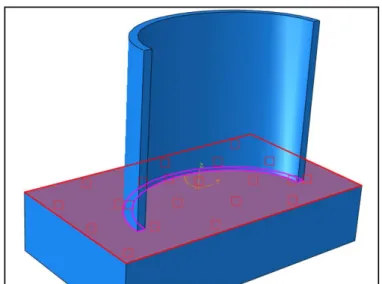
In this section the contact interaction between the build plate and the part is modelled. In the thermal model a “tie” constrain is implemented which unifies the temperatures of the two surfaces in contact. The surface in contact can be visualized at the figure 23. The fixturing losses from the build plate to the machine are ignored. It is a fair modelling choice when the part is relatively small and the build plate does not heat up [7].
The same surface is used to apply the interaction for the structural analysis. Again a “tie” condition is applied, meaning that the nodes belonging to the two components unify their translational motion.
44
6.6.
Printing parameters.
There are different parameters that enable a customization of the printing process. For example, the energy absorption coefficient, the laser energy distribution parameters, the type of element activation or the behaviour of the inactive elements.
An absorption coefficient η equal to 0.46 is selected. This value had the best agreement with experimental results in a previous study of the same material Ti-6Al-4V under the effect of a laser radiation [20]. An accurate value of this parameter is important because it limits proportionally the amount of energy that the part gets from the laser.
The parameters belonging to the Goldak’s spatial energy distribution are summarized in the table 3. They correspond to the melting pool dimensions in millimetre calibrated in Keller’s experimental-simulation work using similar printing conditions [10].
The elements are partially activated to fit the cases when the thickness of the physical powder layer does not match the finite element height. According to the heat energy balance experiment in a unitary element cube, the partial activation keeps accurate temperature results [20].
Finally, the follow deformations option determines whether or not the inactivated elements are allowed to move and follow the predicted deformation of the part. By default, elements that are inactive do not contribute to the overall response of the model and their degrees of freedom are not part of the solution. In stress-displacement analyses this approach works only if displacements are relatively small. If that is not the case, the inactive elements may become excessively distorted before they get activated, which may cause convergence difficulties or produce poor results [21]. Thus, the option is activated. A model validated by the National Institute of Standards and Technology (NIST) activated the deformations [22].
Parameter Value a 0.03 b 0.085 cf 0.03 cr 0.03 ff 1 fr 1
45
6.7.
Cooling.
Convection and radiation are the two heat-transfer mechanism of cooling to the environment. Both are subjected to a sink temperature corresponding to the room temperature of 40 ˚C.
A typical film coefficient h for inert gas atmosphere of 18 W/m2K is set to all the free
surfaces of the model except the bottom surface of the build plate [19]. The key-parameter in the radiation is the emissivity ε of the surface exposed to the atmosphere. The value selected is
0.201 defined in a previous study for the same material and similar process [23].
The cooling is continuously applied during the whole part printing time of 106 seconds and an extra cooling time of 120 seconds.
6.8.
Mesh.
The element used in both thermal and mechanical models is a 3D 8-nodes linear brick element shown at the figure 24. The designation for the heat transfer element is DC3D8 and for the structural element C3D8.
The spatial distribution of the elements is uniform or “mapped” along the printed part. The build plate presents a progressive refinement when getting closer to the part location. The proposed mesh distributions are depicted in figure 25 for the part and build plate.
The size of the elements influences the results of the printing simulation. A convergence study is done in each model to the part mesh in order to obtain accurate results in a reasonable computational time. The studies are described in Appendix A.2.1. resulting in an element size of
0.8 physical layers per element for the HF model and 3 physical layers per element for the MF
model. Consequently, the mesh of the part is formed by 187866 and 11237 nodes for the HF and MF models, respectively.
46
Figure 24: 8 node linear brick element.
Figure 25: Mesh distribution for the part (left) and the build plate (right).
6.9.
Time-stepping
The printing of a single layer is divided in two time periods with very different requirements. The period belonging to the layer deposition and subsequently the laser melting period. The layer deposition takes 1 s and can be modelled with a coarse time step as there is not any change in the temperature trend during this period. A single time increment is implemented.
On the other hand, the laser movement requires a finer time increment to capture the high gradient of temperature along the part cross section. A time stepping convergence study is necessary to select an increment refined enough but avoiding an unfeasible computational cost. The convergence studies of the thermal and mechanical HF solutions are described in Appendix A.2.2. The thermal history evaluation of the part revealed an efficient time increment of 0.75 ms for the HF model and 0.35 s for the MF model.
47
The thermal temperature field of the HF model introduces a huge amount of data in the mechanical model. In order to save computational resources, the mechanical results are evaluated in a reduced model representing the first ten printed layers.
The mesh is the same as in the thermal model in order to avoid extrapolation errors at transferring the temperature between dissimilar meshes. The evaluation of the displacement and stress fields revealed an efficient time increment of 1 ms for the HF model and 0.146 s for the MF model. Both completed convergence studies are described in Appendix A.2.2.
6.10.
Results.
With the proper space and time discretization selected, the sequential thermo-mechanical model is solved. The asymmetric matrix storage and solution scheme is activated to avoid convergence problems caused by the asymmetric system of equations introduced by the temperature-dependent conductivity of the material [9].
6.10.1. Thermal results.
6.10.1.1. High Fidelity model.
The new and refined time step increment increased excessively the magnitude of the temperature using the original power of 250 W. Thus, a calibration of the power is carried out to save energy of the system but ensuring that the material melts (over 1873 K). The result provided a power of 160 W for all the layers except for the first one of 100 W.
The melting pool is analysed for an infill track of the laser path. The large gradient of
temperature caused by the fast movement of the laser is shownin figure 26. The real molten
pool shape is depicted at the figure 27. There is a full melting of the part’s cross section. In addition, the melting pool penetrates the layer underneath causing a partial re-melting.
The temperature history is analysed to have a quantitative and detailed view of how the printing process thermally affects to a point of the part. Figure 28 shows the thermal history of node 971 located at the contour of the fourth layer of the part. The graph is limited to the printing of the first 10 layers. The first heating-cooling cycle is described below: