Abstract
This paper presents a Backtracking Search Optimization algorithm (BSA) to simultaneously optimize the size, shape and topology of truss structures. It focuses on the optimization of these three as-pects since it is well known that the most effective scheme of truss optimization is achieved when they are simultaneously considered. The minimization of structural weight is the objective function, imposing displacement, stress, local buckling and/or kinematic stability constraints. The effectiveness of the BSA at solving this type of optimization problem is demonstrated by solving a series of benchmark problems comparing not only the best designs found, but also the statistics of 100 independent runs of the algorithm. The numerical analysis showed that the BSA provided promising results for the analyzed problems. Moreover, in several cases, it was also able to improve the statistics of the independent runs such as the mean and coefficient of variation values.
Keywords
Backtracking Search algorithm; truss optimization; topology opti-mization; size optiopti-mization; shape optiopti-mization; mixed variable problem
A Backtracking Search Algorithm for the Simultaneous
Size, Shape and Topology Optimization of Trusses
1 INTRODUCTION
Optimization of trusses has been widely studied over the past decades, mostly because of the grow-ing requirement from the industry for more economical design. In fact, several real life structures, or at least part of them, may be modelled using truss elements, such as roofs, towers, bridges, and so on. The difficulty of solving the optimization of truss structures may range from very simple prob-lems to complex ones.
Rafael R. Souza a
Leandro F. Fadel Miguel a Rafael H lopez a
André J. Torii b Letícia F.F. Miguel c
a Center for optimization and Reliability
in Engineering – CORE. Federal Univer-sity of Santa Catarina. R.JoãoPio Du-arte, sn, Florianópolis, SC, 88034-000, Brazil. [email protected], [email protected],
b Federal University of Paraíba. Rua
Castelo Branco, 55.051-900, João Pessoa - PB, Brazil. [email protected]
c Federal University of Rio Grande do
Sul. Av. Sarmento Leite 425, 2º andar, 90050-170, Porto Alegre – RS, Brazil. [email protected]
http://dx.doi.org/10.1590/1679-78253101
For example, a truss size optimization problem with continuous design variables and stress con-straints is a linear and convex problem (considering a unique load case), which is rather simple to be solved. If shape variables are added to the problem, it becomes nonlinear and it may be noncon-vex (Achtziger 2007, Torii et al. 2011, Torii et al. 2012). The difficulty of the problem may be fur-ther increased by including, for example, topology and discrete design variables. The latter usually comes from limitations of the manufacturing process, e.g. the available cross sectional areas in a manufacturer catalogue.
The so-called metaheuristic algorithms, are a class of optimization methods able to handle these difficulties, regarding the truss optimization problems. These algorithms can also be found in differ-ent applications, such as in Rojas et. al. (2012), Koide et. al. (2013), Lobato and Steffen Jr (2014), Behrooz et. al. (2016). Examples of these algorithms are the Genectic Algorithms (GA), Particle Swarm Optimization (PSO), Ant colony (AC) and others.
It is important to point out that lighter structures may be designed when the engineer considers the combined effect of size, shape and topology variables. However, most of the papers found in the literature regarding truss optimization using metaheuristics focused on one or two of these aspects. Indeed, metaheuristic algorithms have been extensively applied to the size optimization of trusses such as Goldberg and Samtani (1986), Adeli and Kamal (1991), and Rajeev and Krishnamoorthy (1992), Bland (2001), Lee et al. (2005), Kaveh and Talatahari (2009a), Kaveh and Talatahari (2009b), Sonmez (2011), Kazemzadeh Azad et al. (2014), Sadollaha et al. (2015), Kaveh and Mah-davi (2014), Kaveh et al. (2014), Degertekin (2012), Degertekin and Hayalioglu (2013), Zhanga et al. (2014), Hasançebi and Kazemzadeh Azad (2014), Kazemzadeh Azad and Hasançebi (2015a), Ha-sançebi and Kazemzadeh Azad (2015), Kazemzadeh Azad and HaHa-sançebi (2014) to name just a few. Papers regarding size and shape optimization can be found at Wu and Chow (1995), Salajegheh and Vanderplaats (1993), Galante (1996), Son and Yang (1996), Jármai et al. (2004), Agarwal and Raich (2006), Kelesoglu (2007), Miguel and Fadel Miguel (2012), Kaveh and Zolghadr (2014), Li (2014), among others.
However, when it comes to the simultaneous size, shape and topology optimization (SSTO) a limited number of papers is found, for example: Pereira et. al. (2004), Tand et al. (2005), Miguel et al. (2012), Miguel et al. (2013), Grierson and Pak (1993), Rajan (1995), Hajela and Lee (1995), Shrestha and Ghaboussi (1998), Deb and Gulati (2001), Ahari et al. (2014), Kaveh and Ahmadi (2014), Kutyłowski and Rasiak (2014), Gonçalves et al. (2015). This fact motivates the development of optimization methods and their application to the SSTO problem.
In this context, a Backtracking Search algorithm (BSA) (Civicioglu 2013. Miguel et al. 2015) is presented in this paper for the simultaneous SSTO of truss structures in the presence of discrete and continuous design variables. The selection of the BSA was mainly based on two aspects:
(a) it was shown to outperform several algorithms in unconstrained optimization (Civicioglu, 2013) and presented promising results for the optimization of transmission line towers struc-tures, studied by Souza et al. (2016);
This paper is organized as follows: in Section 2, the truss optimization problem is stated. In Section 3, the framework of the BSA is presented. Then, a set of benchmark problems regarding the SSTO of trusses is analyzed in Section 4, and finally Section 5 presents the main conclusions drawn from this work.
2 PROBLEM FORMULATION
The problem is formulated similarly to Miguel et al. (2013), where the topology is optimized through a ground structure concept, in which members and nodes are allowed to be eliminated in order to vary the truss topology.
Simultaneously, the algorithm performs the size optimization of the truss by changing the cross-sectional area
(
ÎRm)
A of the remaining structural members and the shape optimization by
modi-fying the nodal coordinates of the nodes q modeled as design variables
(
xÎRq')
. Thisoptimiza-tion procedure searches for the minimum structural weight of the truss subjected to stress, dis-placement and kinematic stability constraints. For convenience of notation, the design variables
A
andx are grouped into the vector
x
A
1,..., , ,...,
A
m
1
q'
. Thus, the optimization problem can be posed as:( )
( )
( )
' 1 max find That minimizesSubject to 1 truss is kinematically stable 2 0, 1,..., G3
m q
m
j j j
j
k k
R
W l A
G
G k q
r x d d + = Î = º
º - £ =
å
x x x( )
( )
1 2tension: 0, or
compression: 0, 1,..., G4 { , ,..., } for discrete variables t j j c j j j np j m
A a a a
s s
s s
º - £
- £ =
º Î W = x
x
min max
min max '
A for continuous variables, 1,..., G5 , 1,...,
j j j
i i i
A A j m
i q
x x x
£ £ =
º £ £ =
(1)
Where
n
v= +
m q
'
which is the number of design variables of the optimization problem, Wstands for the structural weight, m is the number of members in design, ρ is the specific weight of
the bar material, lj is the length of the jth bar (which is represented by the nodal distances). σj is the
stress of the jth bar, while stj and c j
s are respectively the maximum allowable stress in tension and
compression of the jth bar; δk and
d
kmax are the displacement and maximum allowable displacementof the kth node, respectively. Ω is the discrete set comprised by np available cross sectional areas;
min j
and
x
imin andx
imax are the lower and upper bounds of the allowable movement of the ith nodalcoordinate treated as design variable, respectively.
The displacement constraints (G2) are formulated by considering that the deflection in a speci-fied coordinate direction of a node must be lower than an allowable displacement chosen by the designer. Likewise, the stress in the element must be lower than the allowable stress in tension and compression of the material (G3). However, if buckling constraints are included in the formulation, the allowable stress in compression is the lowest value between the maximum stress in compression of the material and the critical stress given by the Euler’s equation (see Eq.(5) in section 5.3). Fi-nally, kinematic stability (G1) is achieved by checking the positive definiteness of the stiffness ma-trix of each solution, by evaluating the determinant of the stiffness mama-trix, i.e. computationally, it should be higher than a very small number, e.g.10-7. If it is not, a penalization of 1020 is applied to this solution. Thus, an unstable design is not analyzed and the constraints according to stress and/or displacement are not evaluated. It is important to highlight that every individual generated by the algorithm is counted as an objective function evaluation, even when the truss analyses is not performed (unstable topologies).
If the stability constraint is satisfied, the member forces and node displacements are calculated. Then, if one or more of the displacement and/or stress constraints are violated (constraints G2 and G3 in Eq. (1)), a penalty Pt is added to the objective function value of the current design. In this
case, the penalty magnitude is proportional to the violation, and takes the form:
max max 1 1
| ( ) |
( )
( )
i m mj j k k
t i
j j j k
P
h
x
x
x
(2)in which
2
,
stands for the absolute value, h is a positive parameter definedaccording to de characteristics and magnitude of each example, i is equal to t if the member is in
tension and i is equal to c if the member is in compression. Finally, constraints on the allowable
cross sectional areas and node positions are addressed by a coding approach. These bounds are im-posed by not sampling infeasible designs in the computer code. Thus, the resulting optimization problem to be solved by the BSA is:
)
(
)
(
)
(
x
x
x
t
P
W
J
(3)3 BACKTRACKING SEARCH ALGORITM (BSA)
The BSA is multi-agent based evolutionary algorithm developed by Civicioglu (2013) able to solve unconstrained non-convex optimization problems. It is thus employed in this paper to address the optimization problem given by Eq. 3.
“direc-tion/length” of the perturbation; the parameter
( )
m
r ; the scale factor aand the matrix M. Becauseof the perturbation process, some variables may extrapolate the boundaries of the design domain; in this case, these variables are randomly regenerated. In the final step, the fitness values are evaluat-ed in order to select the new population. The process is repeatevaluat-ed until the stop criteria is met.
For a more detailed description of the BSA, the reader is referred to Civicioglu (2013) and Sou-za et al. (2016)
1. Initialization Do
Generation of the Perturbed/Trial Population
2. Evaluation of the “direction/length” of the perturbation 3. Perturbation of the current population
end
4. Selection of the new population Untilstop criteria is met
Figure 1: Pseudocode of BSA.
In the original description of the BSA, the author claimed that this algorithm had only one pa-rameter to be adjusted, the mix rate (mr). It was only possible to have this one parameter due to the following aspects: (i) fixing the probability of occurrence of cases 1 and 2 in the construction of both Pold and M, and (ii) fixing the length of the perturbation, i.e. the value of α. Of course, these
parameters may also be adjusted accordingly to the designer needs. In fact, on this paper the mix rate (mr) was kept unchanged from the original version of BSA, while the scale factor a, was the parameter adjusted, based on its performance on each studied example.
4 BSA FOR SIMULTANEOUS TOPOLOGY, SHAPE AND SIZE OPTIMIZATION
The BSA was originally proposed for unconstrained continuous optimization problems. Thus, in order to apply it to a constrained and discrete problem, some modifications are necessary.
The constraints can be divided into two categories: the first one (G1, G2, and G3) regards the structural behavior (Section 2) and the second one (G4 and G5) regards the range of the design variables (Section 2). The former is addressed by the algorithm through a penalization strategy described by Eq. 2 and Eq. 3 of the Section 2. The scheme allows the optimization process to avoid undesirable parts of the domain, penalizing each design proportionally to its violation. The latter is addressed by setting upper and lower bounds to the range of the variables, which will be used by the BSA. Thus, the range is applied on the “Initialization” phase and also at the end of the “Con-struction of the trial or perturbed population Ppert. Hence, the constrained optimization problem
can be transformed in an unconstrained optimization problem.
discrete ones. For instance, in the size optimization, the continuous variables can be rounded into each 1.0 in2 or, still, into an integer value which corresponds to a value on a discrete set of
cross-sectional areas. Then, the BSA only deals with continuous variables. It is important to highlight that this strategy does not demand any modifications on the BSA itself since the operator is applied within the structural analysis code.
Furthermore, this strategy it is easily applicable to any other optimization algorithms originally developed for unconstrained continuous problems. The approach employed on this paper has been successfully applied by other researches, such as Miguel and Fadel Miguel (2012), Miguel et al. (2013) and Gonçalves et al. (2015).
In order to address the simultaneous optimization of size, shape and topology of trusses, a sin-gle-stage procedure is performed, in which all variables including topology, shape and size are de-termined simultaneously. Here, we employed different approaches for eliminating members when the cross-section areas are continuous or discrete. These approaches are detailed in the following.
In the case of continuous cross-sectional areas, during the optimization process, a specific mem-ber is eliminated from the ground structure following the criteria proposed by Deb and Gulati (2001). The cross-sectional area of a member is compared to a specific critical cross-sectional area. If the member area is smaller than this specific value, this element is eliminated from the ground structure. This method defines how different topologies can be obtained in a continuous optimiza-tion procedure. Note that the critical cross-secoptimiza-tional area and the lower (Amin) and upper (Amax) bounds of the cross-sectional areas must be determined by considering the probability of a specific element to be absent from the final solution. For example, if Amin = –Amax and the critical
cross-sectional area is zero, the probability of any member being present in the final structure is approx-imately 50 %.
In the case of discrete cross-sectional areas, the user defines the number of zeros that are added to the available profile set Ω, where a member addressed to a zero cross-sectional area, is eliminated from the ground structure. As well as the values of Amin, Amax and the critical area for the
continu-ous case, the number of zeros added to the set Ω is defined in order to generate a reasonable proba-bility of eliminating an element from the ground structure. It is important to highlight that the supports and nodes carrying loads cannot be disregarded in the final solution.
Finally, the results presented on the following Tables and Figures are feasible solutions (i.e. a solution that respects all the imposed constraints) achieved by the optimization algorithm. The results are compared regarding the weight of the best design, mean value and coefficient of varia-tion of the 100 independent runs. The addivaria-tional informavaria-tion about the best designs (found by the present study and the ones reported in the literature) are presented in the Appendix A.
4.1 Eleven-Bar Truss Example
Design parameter Value
Modulus of elasticity 68947.591 MPa
Weight density 2767.990 kg/m3
Allowable stress in tension 172.396 MPa
Allowable stress in compression 172.396 MPa
Allowable y-displacement 50.8 mm
Table 1: Design parameters for the eleven-bar truss problem.
Figure 2: Eleven-bar truss benchmark example.
This problem was studied by Rajan (1995) and Balling et al. (2006) who employed the GA, Martini (2011) who employed the Harmony Search (HS), and Miguel et al. (2013) who employed the FA. In this study, the truss shape is optimized allowing the vertical coordinates of the three superior nodes (1, 2 and 3, Figure 2) to move between 457.2 cm and 2540 cm. The cross-sectional areas, for each of the 11 bars, come from the discrete set
W
= (0, 0, 0, 0, 0, 0, 0, 0, 0, 0, 10.45159, 11.61288, 15.35481, 16.90319, 18.58061, 19.93544, 20.19351, 1.80641, 23.41931, 24.77414, 24.96769, 26.96769, 28.96768, 30.96768, 32.06445, 33.03219, 37.03218, 46.58055, 51.41925, 74.19340, 87.09660, 89.67724, 91.61272, 99.99980, 103.22560, 121.29008, 128.38684, 141.93520, 147.74164, 170.96740, 193.54800, 216.12860)c m2. Thus, the design vector can be written as[
,
...,
,
,
,
]
3 2 1 11 2
1
A
A
A
x
.Note that the first 10 cross-section areas from the set Ω are null values. Where a member addressed to a null area is eliminated from the structure.
Because the nodal coordinates are continuous variables and the cross-sectional areas are taken from a set of 42 discrete variables, the problem is a mixed variable optimization problem in that it simultaneously addresses discrete and continuous design variables.
The parameters in this example were set as
n
pop=
10
,it
max=
5000
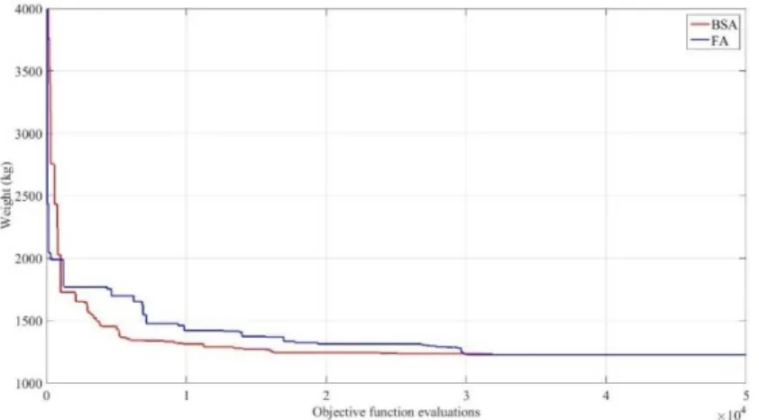
, the penalization term hwas set as 108 and the scale factor α was set as 3 randn, where randn is random number from a standard normal distribution between 0 and 1. The results obtained by the BSA are presented in Table 2 and compared to the results of other algorithms taken from the literature. Figures 3 illus-trates the topology of the optimized structure. Figure 4 showsthe converge curve of the best result found with BSA and FA (Miguel et al. 2013), one can notice that despite the similar results, the BSA converged significantly faster.
Resul Rajan (1995) Balling et. al.
(2006) Martini (2011)
Miguel et. al.
(2013) Present study
OFE 3840 500000 4075 50000 50000
Weight (kg) 1475.999 1241.029 1315.418 1227.04 1227.070
Mean weight - - - 1268.285 1265.654
C.O.V. (%) - - - 2.12 2.02
Table 2: Results for the size, shape and topology optimization of the eleven-bar truss.
Figure 3: Optimized configuration for the size, shape and topology optimization problem of the eleven-bar.
The best result over 100 runs in this study weights 1227.070 kg, which is slightly worse than the value found by Miguel et al. (2013) (1227.040 kg), but better than the optimum weight determined by Balling et al. (2006) (1241.029 kg), Rajan (1995) (1475.999 kg) and Martini (2011) (1315.418 kg). The mean value and COV provided by the BSA are equal to 1265.654 kg and 2.02%, respectively, which are better than the ones found by the FA of Miguel et al. (2013) (1268.285 kg and 2.12%, respectively). Thus, the proposed scheme improved the mean and COV results than the cited refer-ences.
4.2 Thirty-Nine-Bar Two-Tiered Truss Example
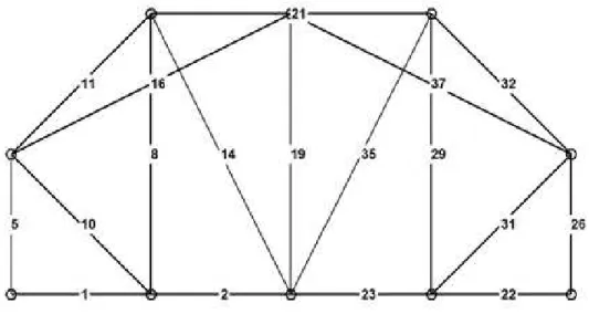
The second benchmark example is the single-span 39-bar, 12-node, simply supported, two-tiered ground structure shown in Figure 5. This structure was studied before by Deb and Gulati (2001), Luh and Lin (2008), Wu and Tseng (2010), Lu and Lin (2011), Miguel et al. (2013) and Ahrari et al. (2014).
Figure 5: Two-tiered truss, thirty-nine-member benchmark example (Miguel et al 2013).
Two independent studies are performed: (i) size and topology optimization and (ii) simultane-ous SSTO. However, the cross-sectional areas are treated as continusimultane-ous variables in this case to properly compare the results to those of the literature. The overlapping members are shown lateral-ly dislocated in the figure for visual clarity. Because the vertical symmetry around member 19 is assumed, the number of variables is reduced to 21. The allowable strength is 137.895 MPa; the ma-terial properties and maximum allowable deflection are the same as those in the previous problem. The stopping criterion is set to OFE = 50000. The BSA parameters employed in both cases were
1/gamrnd(1,0.5), where gamrnd(1,0.5) is a random number from a gamma distribution with shape
parameter 1 and scale parameter 0.5.
4.2.1 Size and Topology Optimization
The procedure for this example consists of the optimization of 21 continuous variables. Each size variable is allowed to vary between -1.4516∙10-4 and 1.45161∙10-3, (in square meters). Where, for values below 3.2258∙10-5, the respective member is eliminated from the ground structure. The design vector can be written
x
[ , ..., ]
A A
1 2A
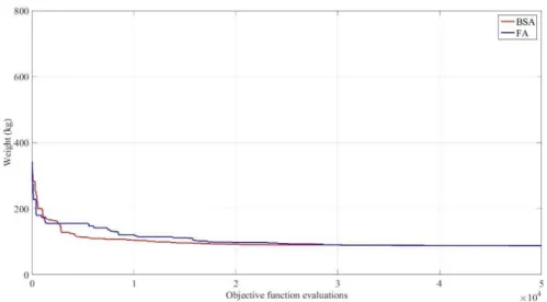
21 . The results found by this study, and others provided by the literature, for this example are listed in Table 3. Figure 6 shows the topology of the best solu-tion given by the BSA, which contains 10 nodes and 18 members. The convergence curves of the BSA and the FA (from Miguel et al. 2013) for this problem are shown in Figure 7.The best result over 100 runs weights 87.637 kg, which is slightly heavier than the 87.549 kg found by Lu and Lin (2011). The mean value obtained using the BSA is equal to 93.284 kg and the coefficient of variation is 5.28%. The coefficient of variation and mean value are only compared with Miguel et al. 2013, since the other studies do not provide this information.
Result Deb and
Gula-ti (2001)
Luh and Lin (2008)
Wu and Tseng (2010)
Lu and Lin (2011)
Miguel et. al. (2013)
Present study
OFE 504000 303600 32300 262500 50000 50000
Weight (kg) 89.152 87.758 87.634 87.549 87.792 87.637
Mean weight (kg) - - - - 100.552 93.284
C.O.V. (%) - - - - 12.9 5.28
Table 3: Results for the size and topology optimization of the eleven-bar truss.
Figure 7: Convergence curves for the size and topology optimization of the thirty-nine-member truss.
4.2.2 Size, Shape and Topology Optimization
To carry out simultaneous SSTO, selected nodal coordinates are taken as design variables in addi-tion to the 21 cross secaddi-tional areas. Assuming symmetry and considering that constrained and load-carrying nodes must remain fixed, and the highest node at the center of the structure does not move laterally, it is possible to reduce the number of nodal coordinates to 7. Each of these 7 nodes is allowed to move (-304.8, 304.8) cm from its original position (Figure 5). The design vector can then be written as:
x
[ , ..., , , ,..., ]
A A
1 2A
21 1 2
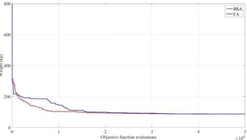
7 .Figure 8 illustrates the topology of the best design found by the BSA over the 100 runs. Note that this topology contains 11 nodes and 20 members. Figure 9 presents the results reached by the present study and others found in the literature are listed in Table 4. The best result over 100 runs achieved by the BSA weights 86.753 kg, which is slightly lighter than the one found by Miguel et al. (2013), but heavier in comparison to the result presented by Ahrari et al. (2014), which is 82.091 kg. The mean value and COV achieved by the BSA optimization scheme are equal to 100.590 kg and 4.60%, respectively, while the ones of the FA are 94.478 kg and 5.3%, respectively. Hence, in this example, the BSA was able to improve the COV.
Result
Deb and Gulati (2001)
Luh and Lin (2008)
Wu and Tseng (2010)
Lu and Lin (2011)
Miguel et. al. (2013)
Ahrari, Atai, and Deb (2014)
Present study
OFE 504000 453600 137200 262500 50000 40256 50000
Weight (kg) 87.176 85.607 85.469 85.541 86.774 82.091 86.753
Mean weight - - - - 94.478 - 100.59
C.O.V. (%) - - - - 5.3 - 4.6
Figure 9 shows the convergence curves for the best results found with the BSA and FA (from Miguel et al. 2013), similarly to previous examples the BSA converged faster, in comparison to the FA. Furthermore, in Figure 10 is shown the convergence curves for the cases 4.2.1 and 4.2.2. Where the better convergence in the earlier iterations for the size and topology case can be associated to the increase of possibilities provided by the geometrical variations allowed in case 4.2.2.
Figure 8: Optimized configuration for the SSTO of the thirty-nine-member truss.
Figure 10: Convergence curves for the size and topology and size, shape and topology optimization of the thirty-nine-member truss.
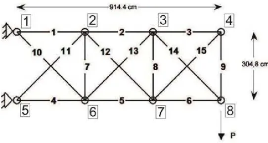
4.3 Fifteen-Bar Planar Truss Example
This fifteen-bar planar truss was studied by Wu and Chow (1995), Tang et al. (2005), Rahami et al. (2008), Miguel et al. (2013) and Gholaizadeh (2013). The ground structure is illustrated in Figure 11, showing a vertical tip load P = 44482.2161 N applied on node 8. The allowable strength of the material is 172.369 MPa for both tension and compression, and the material properties (modulus of elasticity and weight density) are the same as in the previous examples. The x and y coordinates of nodes 2, 3, 6 and 7 and the y-coordinate of the nodes on bar9 are taken as design variables. Howev-er, nodes 6 and 7 are constrained to have the same xcoordinates of the nodes 2 and 3, respectively. Thus, the problem includes fifteen size and eight shape variables (x2=x6, x3=x7, y2, y3, y4, y6, y7, y8).
The cross-sectional areas are chosen from the set
W
= (0.716, 0.910, 1.123, 1.419, 1.742, 1.852, 2.239, 839, 3.477, 6.155, 6.974, 7.5748.600, 9.600, 11.381, 13.819, 17.400,18.064, 20.200, 23.000, 24.600, 1.000, 38.400, 42.400, 46.400, 55.000, 60.000, 70.000, 86.000, 92.193, 110.774, 123.742) cm².The side constraints for the shape variables are 254 cm £ x2 £ 355.6 cm, 558.8 cm £ x3 £
660.4 cm, 254 cm £ y2 £ 355.6 cm, 254 cm £ y3 £ 355.6 cm, 127 cm £ y4 £ 228.6 cm, -50.8 cm £ y6 £ 50.8 cm, -50.8 cm £ y7 £ 50.8 cm, and 50.8 cm £ y8 £ 50.8 cm.
Two independent studies are performed: (i) size and shape optimization, (ii) simultaneous SSTO. On both cases buckling constraints are considered.
For all examples the design vector can be written as
x
[ , ..., , , ,..., ]
A A
1 2A
15 1 2
8 . In order to perform the topology optimization10 null cross-sectional areas are added to the available set Ω. If a size variable Aj assumes a null value, the respective member is eliminated from the structure.The BSA parameters were set in these two studies as npop = 8 and itmax = 1000, resulting in
8000 OFE. The penalization term was set as 108 and the scale factor α was set as 1/gamrnd(1,0.5). The member stresses are constrained to be below the Euler buckling stress, as shown in Eq. 4:
2
8
100
i i cr
L
EA
(4)4.3.1 Size and Shape Optimization with Buckling Constraints
Wu and Chow (1995) and Miguel et al. (2013) have studied this problem using the GA and FA, respectively.
Wu and Chow (1995) carried out the optimization using a population of 30 individuals. Howev-er, they did not mention the maximum number of generations. Miguel et al. (2013) employed 10 fireflies and 800 iterations, resulting in 8000 OFE.
The BSA results together with a comparison with the GA and FA are presented in Table 5. The best design found by the BSA is illustrated in Figure 12. Figure 13 shows the convergence curves of the best results found with the BSA and FA (from Miguel et al. (2013)).
The best results over 100 runs achieved by the BSA weights 59.641 kg, which is lighter than the ones of the GA and FA. The mean value and COV reached by the BSA are equal to 64.049 kg and 3.96%, respectively. Thus, on the one hand, the BSA reduced the mean value of the independent runs in 9.21%, and on the other hand, the COV was around 2.7% higher than the one of the FA.
Result Wu and
Chow (1995)
Miguel et. al. (2013)
Present study
GA FA BSA
OFE - 8000 8000
Weight (kg) 182.506 62.627 59.641
Mean weight - 69.948 64.049
C.O.V. (%) - 3.85 3.96
Figure 12: Optimized configuration for the size and shape optimization with buckling constraint of the 15-bar truss.
Figure 13: Convergence curves for the best result for the size and shape optimization with buckling constraint of the 15-barr truss.
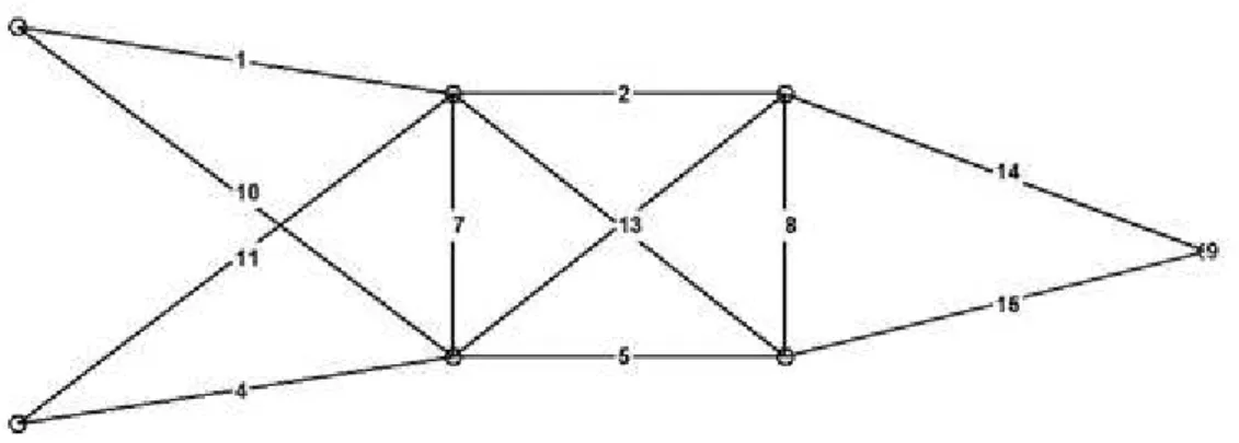
4.3.2 Size, Shape and Topology Optimization with Buckling Constraints
As proposed by Miguel et al. (2013), in addition to the eight discrete size and five continuous con-figuration variables, all fifteen member groups are considered as topology variables in this example. In order to employ the topology optimization, simultaneously to the size and shape optimization, 10 null areas are added to the set of possible cross-sectional areas. Thus, when a null area is addressed, the respective member is eliminated from the structure.
The best design over 100 runs achieved by the BSA weights 54.418 kg, which is 3.48% lighter than the best design provided by the FA. The mean value and COV reached in the present study are equal to 60.187 kg and 7.88%, respectively. Thus, the BSA reduced the mean value by 13.05% and the COV by 0.81%, when compared to the FA. The results for this case show that the BSA was capable of not only provide the lightest design ever found for this problem, but also lower mean and COV values.
Result Miguel et.
al. (2013)
Present study
OFE 8000 8000
Weight (kg) 56.803 54.827
Mean weight 69.223 60.187
C.O.V. (%) 8.69 7.88
Table 6: Results for the size, shape and topology optimization with buckling constraint of the 15-bar truss.
Figure 14: Optimized configuration for the size, shape and topology optimization with buckling constraint of the 15-bar truss.
Figure 16: Convergence curve for the best result for the size and shape and size, shape and topology optimization with buckling constraint of the 15-bar truss.
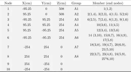
4.4 Twenty-Five-Bar 3D Truss Example
This example was studied before by Rajeev and Krishnamoorthy (1992), Wu and Chow (1995), Tang et al. (2005),Rahami et al. (2008), Miguel et al. (2013), Gholaized (2013) and Ahrari Atai and Deb (2014).The ground structure is shown in Figure 17. The mechanical properties and the loading conditions are presented in Table 7, while the nodes coordinates and member grouping are present-ed in Table 8. The structure is subject to a stress constraint of 275.8 MPa for each member, and a displacement constraint of 0.89 cm for each node.
Mechanical properties
Modulus of elasticity E=68.95 GPa Density of the
materi-al
r
=0.0272N/cm3
Loading (Node) Fx (kN) Fy (kN) Fz (kN)
1 4.454 -44.482 -44.482
2 0 -44.482 -44.482
3 2.224 0 0
6 2.669 0 0
Node X(cm) Y(cm) Z(cm) Group Member (end nodes)
1 -95.25 0 508 A1 1(1,2)
2 95.25 0 508 A2 2(1,4), 3(2,3), 4(1,5). 5(2,6)
3 -95.25 95.25 254 A3 6(2,5), 7(2,4), 8(1,3), 9(1,6)
4 95.25 95.25 254 A4 10(3,6), 11(4,5)
5 95.25 -95.25 254 A5 12(3,4), 13(5,6)
6 -95.25 -95.25 254 A6 14 (3,10), 15(6,7), 16(4,9),
17(5,8)
7 -254 254 0 A7 18(3,8), 19(4,7), 20(6,9),
21(5,10)
8 254 254 0 A8 22(3,7), 23(4,8), 24(5,9),
25*6,10)
9 254 -254 0
10 -254 -254 0
Table 8: Nodes coordinates and member grouping for the twenty-five-bar 3D truss example.
Figure 17: Twenty-five-bar 3D truss example.
During the optimization the cross-sectional areas are chosen from the set
W
= (0.645, 1.290, 1.936, 2.581, 3.226, 3.871, 4.512, 5.161, 5.807, 6.452, 7.097, 7.742, 8.387, 9.032, 9.677, 10.323, 10.968, 11.613, 12.258, 12.903, 13.548, 14.193, 14.839, 15.484, 16.129, 16.774, 18.065, 19.355, 21.935) cm2.Two independent studies were performed: (i) size and shape optimization and (ii) simultaneous size, shape and topology optimization.
The BSA parameters were set in these two studies as npop = 10 and itmax = 600, resulting in
randgis a scalar random value chosen from a gamma distribution with unit scale and shape. The
statistical results presented, for both cases, are extracted from 100 independent runs of the algo-rithm.
4.4.1 Size and Shape Optimization
For the size variation, the member groups are allowed to assume the cross-sectional areas from the set Ω. The x, y, and z coordinates of nodes 3, 4, 5 and 6 and the x and y coordinates of nodes 7-10
are taken as design variables, while nodes 1 and 2 remains unchanged. Due to symmetry of the structure there are five shape variables, with the following bounds: 50.8 cm £ x4£ 152.4 cm,
101.6 cm £ x8£ 203.2 cm, 101.6 cm £ y4£ 203.2 cm, 254 cm £ y8£ 355.6 cm and 228.6 cm
£ z4£ 330.2 cm. Thus, the design vector can be written as
x
= ë
é
A A
1, ,..., , , ,...,
2A
8 1 2x x
x
5ù
û
.The results for this case are presented in Table 9, the best result found with the BSA was 54.02 kg, which slightly worse compared to Miguel et al. (2013) and Gholaized (2013). Figure 18 presents the convergence curves for the BSA and FA and Figure 19 illustrates the best design found with BSA.
Result
Rajeev and Krishnamoorthy
(1992)
Wu and Chow (1995)
Tang et al. (2005)
Miguel et al. 2013
Gholaizedh (2013)
Present study
OFE 6000 6000 8000 6000
Weight (kg) 247.6658 61.7792 56.6718 53.9003 53.1746 54.0189
Mean weight (kg) 60.010 61.8256
C.O.V. (%) 5.5 5.55
Table 9: Results for the size and shape optimization of the Twenty-five-bar 3D truss example.
Figure 19: Optimized configuration for the size and shape optimization of the twenty-five-bar 3D truss example.
4.4.1 Size, Shape and Topology Optimization
In order to perform the topology variation each one of the eight member groups are allowed to be eliminated during the optimization process. To do so, 20 null areas are added to the set of possible cross-sectional areas Ω.
The results for this case are shown in Table 10, the BSA presented a lower C.O.V compared with the FA, however the best result (53.94 kg) and mean weight (66.84 kg) were worst compared to previous works. The configuration of the best result found with the BSA and the convergence curves of the BSA and FA are presented in Figures 20 and 21, respectively. Additionally, Figure 22 presents the convergences curves for the size and shape and size, shape and topology optimization cases. Similarly to the previous examples, the BSA presented a faster convergence in the early itera-tions.
Result
Rajeev and Krishnamoorthy
(1992)
Wu and Chow (1995)
Tang et al. (2005)
Miguel et al. 2013
Gholaizedh (2013)
Present study
OFE 6000 6000 8660 10000 6000
Weight (kg) 61.7792 53.8550 52.8798 51.8986 51.8728 53.9444
Mean weight (kg) 63.1219 66.8429
C.O.V. (%) 8 6.96
Figure 20: Optimized configuration for the size, shape and topology optimization of the twenty-five-bar 3D truss example.
Figure 22: Convergence curve for the best result for the size and shape and size, shape and topology optimization of the twenty-five-bar 3D truss example
5 CONCLUDING REMARKS
This paper presented a Backtracking Search Algorithm (BSA) for the simultaneous SSTO of truss structures. It focused on the optimization of these three aspects since it is well known that the most effective scheme of truss optimization is when one considers them simultaneously. In addition, in most of the examples, we deal concurrently with continuous and discrete design variables, due to the difficulties that they impose.
The effectiveness and robustness of the algorithm were demonstrated through a series of benchmark problems taken from the literature. Not only the best design obtained by each algorithm was compared, but also the statistics of the best designs found over 100 independent runs of the BSA. This statistical analysis is of paramount importance due to the stochastic nature of metaheu-ristic algorithms. Hence, the results presented here may serve as a more formal basis of comparison for future researchers analyzing the same problems with other optimization methods.
From the numerical analysis, it was shown that the BSA provided the best design ever found for several of the analyzed problems. Moreover, in some cases, it was also able to improve the sta-tistics of the independent runs such as the mean and COV values. These results emphasize the ca-pabilities of the BSA in this field and motivate its further development as well its application to real engineering problems.
Acknowledgements
References
Achtziger, W. (2007). On simultaneous optimization of truss geometry and topology. Structural and Multidiscipli-nary Optimization 33: 285–305. DOI 10.1007/s00158-006-0092-0
Adeli, H., Kamal, O. (1991). Efficient optimization of plane trusses. Adv. Eng Softw. 13(3): 116-122.
Agarwal, P and Raich, A.M. Design and optimization of steel trusses using genetic algorithms, parallel computing, and human-computer interaction Structural Engineering and Mechanics.23(4): 325-337.
Ahrari, A., Atai, A.A., Deb, K. (2014). Simultaneous topology, shape and size optimization of truss structures by fully stressed design based on evolution strategy. Eng. Optimiz. DOI:10.1080/0305215X.2014.947972
Balling, R.J., Briggs, R.R., Gillman, K. (2006). Multiple optimum size/shape/topology designs for skeletal structures using a genetic algorithm., J Struct. Eng. 132(7): 1158–1165. DOI:10.1061/ ASCE0733-9445 2006132:7 1158
Behrooz, A., Mohammad, R. K. R., Shahram Y., Mahdi T. (2016) A heuristic algorithm based on line-up competi-tion and gener-alized pattern search for solving integer and mixed integer non-linear optimizacompeti-tion problems. Latin American Journal of Solids and Structures. 13(2).
Bland, J.A. (2001). Optimal structural design by ant colony optimization. Eng Optimiz. 33(4): 425-443. DOI:10.1080/03052150108940927
Civicioglu, P. (2013). Backtracking search optimization Algorithm for numerical optimization problems. Appl. Math. Comp. 219:8121-8144. DOI: 10.1016/j.amc.2013.02.017.
Deb, K., Gulati, S. (2001). Design of truss-structures for minimum weight using genetic algorithms. Finite Elem. Anal. Des. 37: 447-465.
Degertekin, S.O. (2012). Improved harmony search algorithms for sizing optimization of truss structures. Comput. Struct. (92-93): 229-241. DOI: 10.1016/j.compstruc.2011.10.022.
Degertekin, S.O. and Hayalioglu, M.S. (2013). Sizing truss structures using teaching-learning-based optimization. Comput. Struct. (119): 177-188. DOI: 10.1016/j.compstruc.2012.12.011.
Dominguez, A., Stiharu, I., Sedaghati, R. (2006). Practical design optimization of truss structures using the genetic algorithms. Res. Eng. Des. (17): 73–84. DOI: 10.1007/s00163-006-0020-8.
Dorn,W.C., Gomory,R.E., Greenberg, H.J. (1964). Automatic design of optimal structures. J. Mecanique 3: 25-52. Fadel Miguel, L. F., Lopez, R. H., El Hami, A., Miguel, L. F. F. (2012). Firefly Metaheuristics for the Size, Shape and Topology Optimization of Truss Structures. In: Eleventh International Conference on Computational Structures Technology - CST 2012, Dubrovnik.
Galante, M. 1996. Genetic Algorithms as an Approach to Optimize real world structures. Int J Numer. Meth. Eng. (39): 361-82. DOI: 10.1002/(SICI)1097-0207(19960215)39:3<361::AID-NME854>3.0.CO;2-1.
Goldberg, D.E., Samtani, M.P. (1986). Engineering optimization via genetic algorithms. Proceedings of the Ninth Conference on Electronic Computations, ASCE, Birmingham, Alabama, pp. 471-482,
Goncalves, M. S., Lopez, R. H. , Miguel, L. F. F. (2015).Search group algorithm: a new metaheuristic method for the optimization of truss structures. Comput. Struct., 153:165–184. DOI: 10.1016/j.compstruc.2015.03.003.
Grierson, D.E., Pak, W.H. (1993). Optimal sizing, geometrical and topological design using a genetic algorithms. Struct. Optimization (6): 151-9.
Hajela,P., Lee, E. (1995). Genetic algorithms in truss topological optimization. Int. J. Solids Struct 32 (22): 3341-3357.
Hajela,P., Lee, E., Lin,C.Y. (1993). Genetic algorithms in structural topology optimization Topology design of struc-tures. M. P. Bendsoe and C. A. M. Soares, eds., Kluwer Academic, Dordrecht, The Netherlands, 117–133.
Hasançebi, O. and Kazemzadeh Azad, S. (2014). Discrete size optimization of steel trusses using a refined big bang-big crunch algorithm. Eng. Optimiz. 46 (1): 61-83. DOI: 10.1080/0305215X.2012.748047.
Hasançebi, O., Kazemzadeh Azad, S. (2015). Adaptive Dimensional Search: A New Metaheuristic Algorithm for Discrete Truss Sizing Optimization. Computers and Structures. 154, 1-16.
Jármai, K., Snyman, J.A., Farkas, J. (2004). Application of novel constrained optimization algorithms to the mini-mum volume design of planar CHS trusses with parallel chords. Eng. Optimiz. 36 (4): 457-471. DOI: 10.1080/03052150410001686495.
Kaveh, A and Ahmadi, B. (2014). Sizing, geometry and topology optimization of trusses using force method and supervised charged system search. Structural Engineering and Mechanics. 50(3):362-282. DOI: 10.12989/sem.2014.50.3.365
Kaveh, A. and Mahdavi., V.R. (2014). Colliding Bodies Optimization method for optimum design of truss structures with continuous variables. Adv, Eng. Softw. (70): 1-12. DOi: 10.1016/j.advengsoft.2014.01.002.
Kaveh, A. and Talatahari, S. (2009a). Size optimization of space trusses using Big Bang–Big Crunch algorithm. Comput. Struct. (87, 17-18): 1129-1140. DOI: 10.1016/j.compstruc.2009.04.011.
Kaveh, A. and Talatahari, S. (2009b) . Particle swarm optimizer, ant colony strategy and harmony search scheme hybridized for optimization of truss structures. Comput. Struct. (87, 5-6), 267-283. DOI: 10.1016/j.compstruc.2009.01.003.
Kaveh, A. and Zolghadr, A. (2014) A new PSRO algorithm for frequency constraint truss shape and size optimiza-tion. Structural Engineering and Mechanics. 52(3):445-468. DOI: 10.12989/sem.2014.52.3.445.
Kaveh, A., Sheikholeslamib, R., Talataharic, S., Keshvari-Ilkhichib, M. (2014). Chaotic swarming of particles: A new method for size optimization of truss structures. Adv, Eng. Softw. (67): 136-147. DOI: 10.1016/j.advengsoft.2013.09.006.
Kazemzadeh Azad, S., Hasançebi, O. (2014). An Elitist Self-Adaptive Step-Size Search for Structural Design Optimi-zation. Applied Soft Computing, 19, 226-235.
Kazemzadeh Azad, S., Hasançebi, O. (2015a). Discrete sizing optimization of steel trusses under multiple displace-ment constraints and load cases using guided stochastic search technique. Structural and Multidisciplinary Optimiza-tion. 52, 383-404.
Kazemzadeh Azad, S., Hasançebi, O., Saka, M.P. (2014). Guided stochastic search technique for discrete sizing op-timization of steel trusses: A design-driven heuristic approach. Computers and Structures. 134, 62-74.
Kelesoglu., O. (2007). Fuzzy Multiobjective Optimization of Truss-structures using genetic algorithms. Adv. Eng. Softw. (38):717-21. DOI: 10.1016/j.advengsoft.2007.03.003.
Koide, R. M., de França, G.V. Z., Luersen, M. A. (2013) an ant colony algorithm applied to lay-up optimization of laminated composite plates. Latin American Journal of Solids and Structures. 10(3).
Kutyłowski R.a and Rasiak, B.b (2014). The use of topology optimization in the design of truss and frame bridge girders. Structural Engineering and Mechanics. 51(1): 67-88. DOI: 10.12989/sem.2014.51.1.067
Lee, K.S., Geem,Z.W., Lee,S.-H.O. ,Bae,K.-W. (2005). The harmony search metaheuristic algorithm for discrete structural optimization. Eng. Optimiz. 37(7): 663-684.
Li, J-P. (2014). Truss topology optimization using an improved species-conserving genetic algorithm. Eng. Optimiz. 47(1):107-128. DOI: 10.1080/0305215X.2013.875165.
Lobato, F.S., Steffen Jr, V. (2004) Fish swarm optimization algorithm applied to engineering system design. Latin American Journal of Solids and Structures. 11(1)
Lopez, R. H., Luersen, M.A., Cursi, E.S. (2009a). Optimization of laminated composites considering different failure criteria. Compos. Part B-Eng 40:731-740. DOI: 10.1016/j.compositesb.2009.05.007.
Luh, G.C., Lin, C.Y. (2008). Optimal design of truss structures using ant algorithm. Structural and Multidisciplinary Optimization, 36(4), 365-379.
Luh, G.C., Lin, C.Y. (2011). Optimal design of truss-structures using particle swarm optimization. Computers & Structures, 89(23), 2221-2232.
Martini, K. (2011). Harmony Search Method for Multimodal Size, Shape, and Topology Optimization of Structural Frameworks. J. Struct. Eng. 137:11. DOI: 10.1061/(ASCE)ST.1943-541X.0000378.
Miguel, L. F. F.; Fadel Miguel, L. F.; Lopez, R. H. (2015). Simultaneous Optimization of Force and Placement of Friction Dampers Under Seismic Loading. Eng. Optimiz., accepted for publication.
Miguel, L.F.F., Lopez, R.H., Miguel, L.F.F. (2013). Multimodal size, shape and topology optimization of truss struc-tures using the firefly algorithm. Adv Eng. Softw. (56) 23-37. DOI: 10.1016/j.advengsoft.2012.11.006.
Miguel, L.F.F; Fadel Miguel, L. F. (2012) Shape and size optimization of truss structures considering dynamic con-straints through modern metaheuristic algorithms. Expert Systems with Applications. 39, 9458-9467.
Pereira, J. T., Fancello, E. A., & Barcellos, C. S. (2004). Topology optimization of continuum structures with mate-rial failure constraints. Structural and Multidisciplinary Optimization, 26(1-2), 50-66.
Rajan, S. D. (1995). Sizing, shape, and topology design optimization of trusses using genetic algorithms. J. Struct. Eng. 121(10): 1480–1487.
Rajeev, S., Krishnamoorthy,C.S. (1992). Discrete optimization of structures using genetic algorithms, J. Struct. Eng. 118 (5): 1233-1250.
Rojas, J.E., Viana, F. A. C., Rade, D. A., Steffen Jr, V. (2004) Identification of external loads in mechanical sys-tems through heuristic-based optimization methods and dynamic responses. Latin American Journal of Solids and Structures 1(3), 297-318.
Sadollaha, A., Eskandarb, H., Bahreininejadc, A., Kim, J.H. (2015). Water cycle, mine blast and improved mine blast algorithms for discrete sizing optimization of truss structures. Comput. Struct. (149):1-16. DOI: 10.1016/j.compstruc.2014.12.003
Salajegheh, E., Vanderplaats, G. (1993). Optimum design of trusses with discrete sizing and shape variables. Struct. Optimiz. 6:79-85.
Sherestha, S.M., Ghaboussi, J, (1998). Evolution of optimum structural shapes using genetic algorithms. J. Struct. Eng. 123(11): 1331-8.
Šilih,S.,Kravanja, S., Premrov, M. (2010). Shape and discrete sizing optimization of timber trusses by considering of joint flexibility. Adv. Eng. Softw. 41: 286–294. DOI:10.1016/j.advengsoft.2009.07.002.
Soh., C.K., Yang, J. (2005). Improved genetic algorithm for design optimization of truss structures with sizing, shape and topology variables. Int. J. Numer. Meth. Eng. (62):1737-1762.
Sonmez, M. (2011). Discrete optimum design of truss structures using artificial bee colony algorithm. Struct. Multi-discip. O. 43:85-87. DOI 10.1007/s00158-010-0551-5.
Souza, R.R., Miguel, L.F.F., Lopez, R.H., Miguel, L.F.F, Torii, A.J. (2016) A procedure for the size, shape and to-pology optimization of transmission line tower structures. Engineering Structures, 111, 162-184.
Tang, W., Tong,L., Gu,Y., (2005). Improved genetic algorithm for design optimization of truss structures with sizing, shape and topology variables. International Journal for Numerical Methods in Engineering 62:1737–1762.
Tang. W., Tong. L., Gu, Y., (2005). Improved genetic algorithm for design optimization of truss structures with sizing, shape and topology variables. Int. J. Numer. Meth. Eng (62) 1737–1762.
Torii, A. J.; Lopez, R. H.; Biondini, F. (2012). An approach to reliability-based shape and topology optimization of truss structures. Eng. Optimiz. (Print) 44: 37-53. DOI: 10.1080/0305215X.2011.558578.
Wu, C.Y., Tseng, K.Y. (2010). Truss structure optimization using adaptive multi-population differential evolution. Structural and Multidisciplinary Optimization, 42(4), 575-590.
Wu, S.J., Chow,P.T., (1995). Integrated discrete and configuration optimization of trusses using genetic algorithms. Comput. Struct. 56(4):695–702.
Zhanga, Y., Houa, Y. and Liua, S. (2014). A new method of discrete optimization for cross-section selection of truss structures. Eng. Optimiz. 46(8): 1052-1073. DOI: 10.1080/0305215X.2013.827671.
APPENDIX A
On this section, the information regarding the best designs, for the studied examples, are presented on the following Tables.
Design variables Rajan
(1995)
Balling et. al. (2006)
Martini (2011)
Miguel et. al. (2013)
Present study
y1 (m) 19.987 - - - 20.057
y2 (m) 14.084 - - - 12.384
y3 (m) 4.7371 - - - -
Member
2 74.193 - - 74.193 74.193
3 23.226 - - 18.581 18.581
4 74.193 - - 37.032 37.032
5 63.871 - - 74.193 74.193
6 9.677 - - 46.581 46.581
8 67.097 - - - -
9 77.419 - - 87.097 87.097
10 60.645 - - - -
OFE 3840 500000 4075 50000 50000
Weight (kg) 1475.999 1241.029 1315.418 1227.040 1227.070
Mean weight - - 1268.285 1265.654
C.O.V. (%) - - 2.12 2.02
Design variables
Deb and Gulati (2001)
Luh and Lin (2008)
Wu and Tseng (2010)
Lu and Lin (2011)
Miguel et al. (2013)
Present study
1 - 0.329 0.323 0.252 0.323 0.323
2 4.845 4.845 4.839 4.839 4.854 5.152
3 0.329 - - - - -
5 9.69 9.690 9.677 9.677 9.678 9.678
7 0.335 - - - - -
8 1.619 1.613 1.613 1.613 1.615 1.3
9 0.329 - - - - -
10 6.845 6.852 6.839 6.845 6.869 7.285
11 6.858 6.858 6.839 6.845 6.846 5.516
14 3.606 3.613 3.606 3.613 3.615 2.907
16 - - - 1.399
19 - - - 1.251
21 6.484 6.452 6.452 6.452 6.462 5.201
22 - 0.329 0.323 0.252 0.323 0.323
23 4.845 4.845 4.839 4.839 4.854 5.152
25 0.329 - - - - -
26 9.69 9.690 9.677 9.677 9.678 9.678
28 0.335 - - - - -
29 1.619 1.613 1.613 1.613 1.615 1.3
30 0.329 - - - - -
31 6.845 6.852 6.839 6.845 6.869 7.285
32 6.858 6.858 6.839 6.845 6.846 5.516
35 3.606 3.613 3.606 3.613 3.615 2.907
37 - - - 1.399
OFE 504000 303600 32300 262500 50000 50000
Weight (kg) 89.152 87.758 87.634 87.549 87.792 87.637
Mean weight - - - - 100.552 93.284
C.O.V. (%) - - - - 12.9 5.28
Design variables Deb and Gulati (2001) Luh and Lin (2008) Wu and Tseng (2010) Lu and Lin (2011) Miguel et al. (2013) Ahrari, Atai and Deb (2014) Present study
1 3.839 2.110 1.052 2.090 1.901 0.596102 2.879
2 7.523 7.065 9.735 7.058 6.87 6.321323 6.435
3 - - - 7.844571 2.575
4 - - - - 7.686 7.110805 -
5 10.419 9.923 5.774 9.903 - 9.695815 10.112
6 - - - 3.610361 1.259
7 - - - 6.779051 0.336
8 0.329 0.523 1.097 - 8.1 - -
10 7.452 7.877 7.245 7.877 - 5.310751 6.089
11 3.252 8.123 7.323 8.116 - 0.322935 5.483
12 - - - 0.529 - - 3.437
14 8.342 3.387 3.503 3.387 0.326 2.334415 -
15 - - - - 9.887 - -
19 - - - - 6.200 2.009196 -
20 - - - 2.29
21 8.761 8.103 7.135 8.097 - - 5.351
22 3.839 2.110 1.052 2.090 1.901 0.596102 2.879
23 7.523 7.065 9.735 7.058 6.87 6.321323 6.435
24 - - - 7.844571 2.575
25 - - - - 7.686 7.110805 -
26 10.419 9.923 5.774 9.903 - 9.695815 10.112
27 - - - 3.610361 1.259
28 - - - - 6.779051 0.336
29 0.329 0.523 1.097 - 8.1 - 6.089
31 7.452 7.877 7.245 7.877 - 5.310751 -
32 3.252 8.123 7.323 8.116 - 0.322935 5.483
33 - - - 0.529 - - 3.437
35 8.342 3.387 3.503 3.387 0.326 2.334415 -
36 - - - - 9.887 - -
OFE 504000 453600 137200 262500 50000 40256 50000
Weight (kg) 87.176 85.607 85.469 85.541 86.774 82.091 86.753
Mean weight (kg) - - - - 94.478 - 100.59
C.O.V.(%) - - - - 5.3 - 4.6
Design variables Wu and Chow (1995) Miguel et al. (2013) Present study Design variables Wu and Chow (1995) Miguel et al. (2013) Present study
GA FA BSA GA FA BSA
A1 38.4 7.574 7.574 A13 8.6 8.6 8.6
A2 11.381 6.974 6.974 A14 11.381 1.852 2.839
A3 9.6 2.839 1.742 A15 11.381 8.6 6.155
A4 38.4 11.381 13.819 X2 301.98314 278.27986 334.33883
A5 13.819 9.6 8.6 X3 565.32526 571.15964 590.35225
A6 9.6 6.974 7.574 Y2 274.3708 262.41248 254
A7 18.064 0.716 0.716 Y3 315.13272 255.1049 254
A8 8.6 1.419 0.716 Y4 139.2809 131.00304 132.36646
A9 2.239 9.6 1.852 Y6 0.88138 43.3324 50.8
A10 6.974 1.123 0.91 Y7 39.41064 48.31588 50.8
A11 8.6 1.419 0.716 Y8 88.16594 124.06884 132.1094
6.974 1.742 1.123
OFE - 8000 8000
Minimum weight (kg) 182.506 62.627 59.641
Mean weight (kg) - 69.948 64.049
C.O.V. (%) - 3.85 3.96
Table A4: Cross sectional area (cm²) and weight (kg) for the size and shape optimization with buckling constraint of the 15-bar truss, on Section 5.3.1.
Design variables
Miguel et al. (2013)
BSA Design
variables
Miguel et
al. (2013) BSA
A1 6.155 6.155 A13 11.381 0
A2 6.155 6.155 A14 3.477 0
A3 0.716 6.155 A15 0 11.38
A4 13.819 13.819 X2 335.26984 322.4111
A5 6.974 8.6 X3 594.3219 561.5408
A6 8.6 0.91 Y2 293.11854 254
A7 0.716 1.742 Y3 296.89552 254
A8 1.419 3.478 Y4 134.7851 139.9969
A9 7.574 2.839 Y6 35.39998 -9.4016
A10 2.839 2.839 Y7 29.4767 50.8
A11 0 0 Y8 131.8133 138.7773
A12 0 1.742
OFE 8000 8000
Weight (kg) 56.803 54.827
Mean weight (kg) 69.223 60.187
C.O.V. (%) 8.69 7.88
Design variables Rajeev and Krishnamoorthy (1992) Wu and Chow (1995) Tang et al. (2005) Miguel et al. 2013 Gholaizedh (2013) Present study
A1 0.6452 0.6452 0.6452 0.6452 0.6452 0.6452
A2 11.6129 1.2903 0.6452 0.6452 0.6452 0.6452
A3 14.8387 7.0968 7.0968 5.8064 6.4516 5.8064
A4 1.2903 1.2903 0.6452 0.6452 0.6452 0.6452
A5 0.6452 1.9355 0.6452 0.6452 0.6452 0.6452
A6 5.1613 0.6452 1.2903 0.6452 0.6452 0.6452
A7 11.6129 1.2903 1.2903 0.6452 0.6452 0.6452
A8 19.3548 5.8064 4.5161 6.4516 5.8064 6.4516
X4 104.3178 90.0938 94.7928 93.8530 90.8948
Y4 135.8138 153.3398 141.5796 138.6332 149.5881
Z4 316.4840 327.8378 321.6148 330.1238 310.1078
X8 129.0320 114.4524 127.3556 131.3942 127.4500
Y8 333.9592 348.0816 346.4560 354.4062 350.3897
OFE 6000 6000 8000 6000
Weight (kg) 247.6658 61.7792 56.6718 53.9003 53.1746 54.0189
Mean weight (kg) 60.010 61.8256
C.O.V. (%) 5.5 5.55
Table A6: Results for the size and shape optimization of the Twenty-five-bar 3D truss example.
Design variables Rajeev and Krishnamoorthy (1992) Wu and Chow (1995)
Tang et al. (2005) Miguel et al. 2013 Gholaizedh (2013) Present study
A1 0.6452 0.0000 0.0000 0.0000 0.0000 0.0000
A2 1.2903 0.6452 0.6452 0.6452 0.6452 0.6452
A3 7.0968 5.8064 7.0968 6.4516 5.8064 6.4516
A4 1.2903 0.0000 0.0000 0.0000 0.0000 0.0000
A5 1.9355 0.0000 0.0000 0.0000 0.0000 0.0000
A6 0.6452 0.6452 0.6452 0.6452 0.6452 0.6452
A7 1.2903 0.6452 0.6452 0.6452 0.6452 1.2903
A8 5.8064 7.0968 5.8064 5.8064 6.4516 5.8064
X4 100.3554 97.7900 98.7298 98.5266 92.2427
Y4 178.2572 163.4490 156.2608 167.9194 136.4609
Z4 267.1064 286.6898 302.7172 286.9692 324.5994
X8 140.0810 124.7902 125.5014 123.9266 112.7463
Y8 346.1258 342.7476 355.0768 352.7806 350.6709
OFE 6000 6000 8660 10000 6000
Weight (kg) 61.7792 53.8550 52.8798 51.8986 51.8728 53.9444
Mean weight (kg) 63.1219 66.8429
C.O.V. (%) 8 6.96