Braz. J. Chem. Eng. vol.24 número3

ISSN 0104-6632 Printed in Brazil

www.abeq.org.br/bjche

Vol. 24, No. 03, pp. 399 - 409, July - September, 2007

Brazilian Journal

of Chemical

Engineering

DISCRETISATION OF THE NON-LINEAR HEAT

TRANSFER EQUATION FOR FOOD FREEZING

PROCESSES USING ORTHOGONAL

COLLOCATION ON FINITE ELEMENTS

E. D. Resende

, T. G. Kieckbusch

, E. C. V. Toledo

and M. R. W. Maciel

1

Universidade Estadual do Norte Fluminense Darcy Ribeiro, Centro de Ciências e Tecnologias Agropecuárias, Laboratório de Tecnologia de Alimentos, UENF/CCTA/LTA,

Phone +(55) (22) 2726-1461, Fax + (55) (22) 2726-1549, Av. Alberto Lamego 2000, Parque Califórnia, CEP: 28013-602, Campos dos Goytacazes - RJ, Brazil.

E-mail: [email protected] 2

Universidade Estadual de Campinas, Faculdade de Engenharia Química, Departamento de Termofluidodinâmica, UNICAMP/FEQ/DTF, Campinas - SP, Brazil.

3

Universidade Estadual de Campinas, Faculdade de Engenharia Química, Departamento de Processos Químicos, UNICAMP/FEQ/DPQ/ LDPS,

Campinas - SP, Brazil.

(Received: March 20, 2006 ; Accepted: June 05, 2007)

Abstract - The freezing process is considered as a propagation problem and mathematically classified as an “initial value problem.” The mathematical formulation involves a complex situation of heat transfer with simultaneous changes of phase and abrupt variation in thermal properties. The objective of the present work is to solve the non-linear heat transfer equation for food freezing processes using orthogonal collocation on finite elements. This technique has not yet been applied to freezing processes and represents an alternative numerical approach in this area. The results obtained confirmed the good capability of the numerical method, which allows the simulation of the freezing process in approximately one minute of computer time, qualifying its application in a mathematical optimising procedure. The influence of the latent heat released during the crystallisation phenomena was identified by the significant increase in heat load in the early stages of the freezing process.

Keywords: Freezing process; Modelling; Heat load; Numerical method.

INTRODUCTION

Freezing is a well-known preservation method widely used in the food industry. Realistic mathematical approaches to freezing process predictions, however, were developed only a few decades ago. The freezing process may be considered as a propagation problem, also called a “march problem,” and mathematically known as an “initial value problem.” The mathematical formulation comprises a complex condition of heat

transfer simultaneously with phase change (Stefan problem), variation in thermal properties and sometimes anisotropy due to the food structure (Delgado and Sun, 2001). The models used to predict freezing time vary from analytical simple equations to numerical methods. The most realistic physical model for freezing is that of non-linear unsteady heat conduction with variable thermal properties and surface convective cooling (Cleland et al., 1987).

refrigeration requirements for freezing systems and to design the equipment necessary for effective and rational processing. Minimisation of the energy requirement, reliability, safety and quality of the product must also be considered. In the quality enhancement process, maximisation of consumer acceptability can be used to optimise process parameters such as rate of freezing or storage conditions (Shewfelt et al., 1997).

It is recognised that the quality of frozen products is largely dependent on the rate of freezing. Slow freezing generally causes undesirable higher ice crystals to form exclusively in extracellular areas, while high freezing rates produce small crystals, evenly distributed throughout the tissues. As a result the equipment designer has to compromise between a freezing rate that minimises process cost and operating conditions that assure appropriate product quality (Delgado and Sun, 2001).

Heat Transfer Models

Numerical methods are regularly used to model heat transfer during food freezing processes. The advantage of numerical methods over simple equations is that the effects of phase change over a range of temperatures, changing thermal properties and heterogeneity of food products can be considered. If numerical methods are formulated and implemented correctly to reduce truncation and rounding errors, they are generally considered the most accurate, reliable and versatile freezing and thawing time prediction methods (Cleland et al., 1987).

In numerical methods the heat diffusion equation can be expressed in the following two ways (Pham, 1985):

( )

T

T C (T) div [k(T) grad(T)]

t ∂

ρ =

∂ (1a)

and

H

div [k(H) grad(T(H))] t

∂ =

∂ (1b)

The first equation uses temperature as the only dependent variable, while the second one represents the enthalpy methods, which have two dependent variables, enthalpy being the primary and temperature the secondary variable. In the first equation, the latent heat is represented by a large but finite wide peak of the curve Cp vs. T. If the time

increments adopted are large, the temperature at the node may cross the range of temperatures at which freezing occurs in a single step. Thus, it bypasses the latent heat load and the total time calculated is shorter than the actual one. To avoid this error very small time increments must be used. The enthalpy method requires either an explicit technique with the consequent problem of convergence, or implicit procedures in which iteration at each time step is used, consuming more computational time.

The techniques used in numerical methods are finite difference (FDM), finite element (FEM), and boundary element and finite control volume. The first two techniques are most frequently used. The potential contribution of the boundary element technique is significant, but until now it has only been applied to a limited number of food and agricultural engineering problems (Puri and Anantheswaran, 1993).

Cleland and Earle (1984) considered various finite difference schemes for phase change problems and concluded that Lee`s implicit, three-time-level scheme was the most accurate. Formulations of both FDM and FEM based on Lee`s scheme have been developed and implemented to predict freezing and thawing for a range of solid geometries (Cleland et al., 1987). In order to be able to include volumetric expansion during freezing, Sheen and Hayakawa (1990) developed a new FDM for irregular domains by applying the alternate direction implicit (ADI) central difference and finite volume methods. The model could be used for simulating different thermal processes of heat conduction in foods.

Several authors have used the finite element method. For unidirectional and regular geometry problems, FEM does not confer a greater advantage than the finite difference technique (Ramaswamy and Tung, 1984; Chau and Gaffney, 1990). Moreover, by applying the numerical grid generation approach, the FDM can be used for irregular geometry as effectively as the more complicated FEM without sacrificing its simplicity (Ansari, 1999). Both FDM and FEM are widely used as tools to develop simple predictive models.

An alternative approach to the FEM is the boundary-fitted grid (BFG) method used by Califano and Zaritzky (1997). The technique was applied to simulate the freezing process in two-dimensional systems of arbitrary shape. The results indicate accuracy similar to that of finite element formulation, combined with a very short computer time and small memory requirements.

(1994) analysed food freezing in a plate freezer by using a PC-based finite element package. The prediction agreed reasonably well with measured data, which validates the applicability of the computer program for simulating the freezing process.

Although commercial packages are constantly being upgraded, simple and fast predictive methods are still preferred by the industry. This may be attributed to the difficulties in finding appropriate product properties and computational conditions. Thus, the development of simple and accessible software would be helpful (Delgado and Sun, 2001). The objective of the present work is to solve the non-linear heat transfer equation for food freezing processes using orthogonal collocation on finite elements (Finlayson, 1980). This technique has not yet been applied to food freezing processes and represents an alternative numerical approach in this area. The model considers the one-dimensional freezing problem as applicable, for instance, to a plate freezer.

DELINEATION OF THE ONE-DIMENSIONAL FREEZING PROBLEM

Most foods have high water content in the form of an aqueous solution embebbing a biopolymeric matrix. Throughout the freezing process, water is gradually transformed into ice crystals, increasing the solute concentration of the remaining solution and causing a continuous depression of the freezing point of the unfrozen matrix. Water and ice differ considerably in specific heat, thermal conductivity and density, and as a consequence, there is a strong dependence of the thermal properties upon the freezing temperature. Since food materials freeze over a range of temperatures, the associated latent heat can be added to the normal heat capacity, yielding an equivalent heat capacity. The variation in the thermal properties and the decreasing freezing temperature of the solution make the process a highly non-linear mathematical problem (Saad and Scott, 1997).

Considering the one-dimensional freezing of an infinite slab of a food material, a mathematical description of the problem can be formulated using the one-dimensional transient heat conduction equation with variable coefficients and symmetric convective boundary conditions, as shown below:

p

T T

(T)C (T) k(T)

t x x

∂ ∂  ∂ 

ρ = _{ }

∂ ∂  ∂  0<x<L, t>0 (2a)

T(x,0) = Ti, 0<x<L, t=0 (2b)

x 0 T

k(T) h(T(0, t) T )

x ₌ ∞

∂

− = −

∂ , x=0, t>0 (2c)

0 x

T k(T)

L x

= ∂

∂ −

= _{, x=L, t>0 (2d)}

where T is the temperature, x is the position, t is the time, k is the thermal conductivity, ρ is the density, Cp is the apparent specific heat, h is the heat transfer

coefficient and L is the half-thickness of the slab. The subscripts i and ∞ indicate respectively the initial and freezing plate temperatures. The thermal properties are functions of temperature and the basic composition of the food.

Thermal Physical Properties

Partially frozen meat products are basically constituted of ice, water and dry fibers. The thermal physical properties of the product can be calculated as a function of frozen water fraction (w), according to the cryoscopic depression model obtained by Mascheroni and Calvelo (1978):

o T

w E F

T T

 

= −  ₋ 

  (3a)

where

b X E 1

X

= −

;

0 DRT F

1000 X

= λ

Density

o o o a

a h (w)

Y

1 w ( 1)

ρ

ρ =

ρ ρ

+ −

ρ ρ

(3b)

Apparent Specific Heat

p

p po o

p

o o o

C (w) C wY C

dw

Y [ C (T T )]

dT

= − ∆ −

λ + ∆ −

Thermal Conductivity

The model proposed by Mascheroni et al. (1977) is a function of temperature and also consider the direction of the fibers inside the meat. Thus, during freezing in the radial and parallel directions to the fibers, the thermal conductivity is given by

2

h h

2 t

t h

k(w) k (1 )[k

4 (1 )

k (1 ) ]

1/k 1/k

= λ + − λ λ +

λ − λ − λ +

+

(3d)

where

o h

1 1 wY /

λ = − − ρ ρ ;

a c t c

1 (1 k /k )

k k

1 ( 1)

− − α β

=

+ α − β ;

c c a

3k /(2k k )

α = + ;

o o a

o o a

(1 w)(Y / )

1 w(Y / )

− ρ ρ

β =

− ρ ρ

Table 1: Fundamental parameters of meat (Yo = 0.7336)

based on Mascheroni and Calvelo (1980)

Bound water = 0.1965 kg water/kg total solids

Solute content in the dry matter (D) = 1.455 moles/kg

Thermal conductivity of unfrozen meat = 0.5057 W/mK

Thermal conductivity of the fibers = 0.3539 W/mK

Density of unfrozen meat = 1053 kg/m3 Specific heat of unfrozen meat = 3.475 kJ/kgK

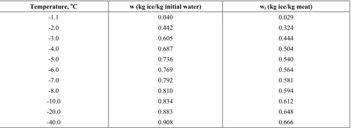
The equations derived by Mascheroni and Calvelo (1980) were used to model the thermal physical properties of meat as a function of temperature. The values of the fundamental parameters used are those determined experimentally by the authors for a 73.36% total initial moisture content and are given in Table 1. The calculated ice fraction is given in Table 2 and indicates that the freezing starts at -1.1oC and that even at -40oC a

fraction of the water that corresponds to the bound water remains unfrozen.

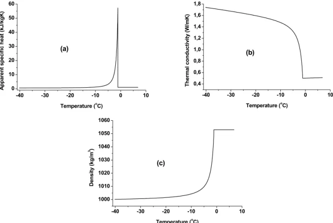
The calculated values for the thermal conductivity, apparent specific heat and specific gravity of the meat under freezing conditions are given in Figure 1a, 1b and 1c, respectively. The strong non-linearity at the initial freezing temperature of the meat is quite evident due to the high ice formation rate, which levels off at temperatures lower than -5oC.

Table 2: Equilibrium fraction of ice at different freezing temperatures

Temperature, oC w (kg ice/kg initial water) wi (kg ice/kg meat)

-1.1 0.040 0.029

-2.0 0.442 0.324

-3.0 0.605 0.444

-4.0 0.687 0.504

-5.0 0.736 0.540

-6.0 0.769 0.564

-7.0 0.792 0.581

-8.0 0.810 0.594

-10.0 0.834 0.612

-20.0 0.883 0.648

-40 -30 -20 -10 0 10 0

10 20 30 40 50 60

(a)

A

ppare

nt

spe

c

if

ic heat

(

k

J

/kgK

)

Temperature (oC)

-40 -30 -20 -10 0 10

0,4 0,6 0,8 1,0 1,2 1,4 1,6 1,8

(b)

T

h

e

rm

a

l c

o

ndu

c

ti

v

ity

(W

/m

K

)

Temperature (oC)

-40 -30 -20 -10 0 10

1000 1010 1020 1030 1040 1050 1060

(c)

D

e

nsity

(kg/m

3 )

Temperature (oC)

Figure 1: Thermal physical properties of the meat as a function of temperature: apparent specific heat (a), thermal conductivity (b), density (c)

Numerical Approach

The heat transfer equations (Equation 2a to 2d) can be written in dimensionless form taking the non-linearity of the thermal physical properties into account (Mascheroni and Calvelo, 1980).

2 *

* * *

2 k

f ∂η= ∂ _k ∂η_=k ∂ η ∂+ ∂η

∂τ ∂ξ ∂ξ ∂ξ ∂ξ ∂ξ (4a)

1

τ = η =1 0≤ ξ ≤1 (4b)

1

ξ = k*∂η=Bi(η −1)

∂ξ τ >0 (4c)

0

ξ = ∂η=0

∂ξ τ >0 (4d)

The related dimensionless variables are

i i

T T

T T_∞

− η =

− ;

x L

ξ = ; o

2 o po

k t C L τ =

ρ

*

o k k

k

=

;

o hL Bi

k

=

and f*, derived by Mascheroni and Calvelo (1980), accommodates the non-linearity of the thermal physical properties as a strong function of the local temperature and therefore depends on the progression of the freezing process:

2

i f i

*

i f i

a b/ ( +

)-f

d g/ | ( + )- |

+ η η η η

=

− η η η η (6)

where

p o po o o po o

o o a

a h

o o a

a h

i i o o f i o

a 1 C Y (E F)/C ; b Y F/C T ;

Y

d 1 ( 1)(E F);

Y

g F ( 1);

(T T )/T ; (T T )/T_∞

= − ∆ + = λ

ρ ρ

= + − +

ρ ρ

ρ ρ

= −

ρ ρ

η = − η = −

The heat transfer equation was discretised along the spatial position using the numerical method of orthogonal collocation on finite elements (Finlayson, 1980). Initially the orthogonal collocation matrixes, Ai,K,l and Bi,K,l, representing the roots of the

orthogonal polynomial of Jacobi are calculated. These matrixes are used as coefficients of the partial differential equations describing the freezing process, allowing specification of the grid of the collocation roots, i, inside each finite element, l, indexed by k nodes in the element. Thus it is possible to use a flexible number of finite elements and collocation roots more compatible with solution of the equation system.

The temperature historic inside the product can be expressed according to the following model:

+

=

 _η 

 η + 

 η 

∂η _{ }

=   ∂τ η η   η      

∑

i, k, l k,l *

CR 2 _i,l i,l

* 2

k 1

i, k, l k,l i, k, l k, l *

i,l

k ( ) B f ( )

1

A k ( )(A ) f ( )

where

i = 2, CR+2 (CR = number of collocation roots) l = 1, FE (FE = number of finite elements)

The boundary conditions can be described as follows:

0

ξ =

(

)

CR 2

l, k ,1 k, l 1,1

k 1

A Bi 1

+

=

η = η −

∑

1 ξ = CR 2 FE,k,FE k,FE k 1 A 0 + = η =

∑

The heat flow balance and the temperature between finite elements are considered as:

+ +

+ + +

= =

η = η

∑

∑

CR 2 CR 2

CR 2,k,l k,l 1,k,l 1 k,l 1

k 1 k 1

A A (11)

The numerical set-up (Equation 8 to 11) is integrated over time applying a numerical solver (DASSL) that allows variable step integration, useful and necessary in the numerical approach to food freezing systems due to the steep change in thermal

properties. This software also permits the integration of the coupled system, simultaneously composed of algebraic and of differential equations, enabling calculation of the temperature grid as a function of time, η(τ)i,l.

The dimensionless instantaneous heat load (φ) as a function of time is evaluated by summation of the instantaneous heat load over all the spatial positions (xi), using the temperature grid calculated after each

time step as well as the respective thermal properties of the mass element, as shown in Equation (12).

+

= =

 

ϕ τ =

∑ ∑

FE CR 2 *

k,l k,l l 1 k 1

( ) f ( ( ) ) ( ) (12)

Thus, the instantaneous heat load for one kilogram of meat can be calculated as follows:

*

k, o po

FE CR 2

1 k 1

[(f ( ( ) ) C ) /

(t) [Temp(k, , t)]](A x)

Temp(k, , t) [Temp(k, , t)] +

= =

 _{η τ ρ} 

 

 

φ = _ρ δ _

  ρ    

∑ ∑

where δx = Lδξ, Temp(k,l,t) = Ti – (Ti – T∞) (η(τ)k,l),

A = 1.0 / Lρo and ρo and Cpo are the density and

specific heat of unfrozen meat, respectively.

The total heat load that evolved in the freezing process is evaluated by integration of the instantaneous heat load, as indicated in Equation (14), making it possible to evaluate the energy spent in the freezing operation.

t 0

(t) (t) dt

Φ = φ_∫ (14)

MODEL VALIDATION

0 ,0 0 ,2 0 ,4 0 ,6 0 ,8 1, 0

0 10 20 30 40 50 60 70

1.0 0.8

0.6 0.4

0.2 0.0

Finite difference method (Mascheroni & Calvelo, 1980) Experimental data (Mascheroni & Calvelo, 1980) 1 FE and 5 CR - computation time = 1.52 min 1 FE and 6 CR - computation time = 1.54 min 1 FE and 13 CR - computation time = 1.7 min 1 FE and 50 CR - computation time = 2.08 min 1 FE and 200 CR - computation time = 52.8 min

C

h

a

ract

eri

st

ic t

im

e (

m

in

)

Position, ξ

Figure 2: Characteristic time calculated for different configuration grids of collocation roots (CR) applied to one finite element (FE) [Operating conditions: Ti = 8.6 oC, T∞ = -44.3 oC, Bi = 18.489]

0,0 0,2 0,4 0, 6 0,8 1, 0

0 10 20 30 40 50

1.0 0.8

0.6 0.4

0.2 0.0

Finite Difference Method (Mascheroni & Calvelo, 1980) Experimental data (Mascheroni & Calvelo, 1980) 3 FE and 2 CR (computation time = 1.65 min) 10 FE and 2 CR (computation time = 1.70 min) 100 FE and 2 CR (computation time = 3.73 min)

Charact

eri

s

ti

c t

im

e

(

m

in

)

Position, ξ

Figure 3: Characteristic time calculated for different configuration grids of finite elements (FE) fixing two collocation roots (CR) [Operating conditions: Ti = 8.6oC, T∞ = -44.3oC, Bi = 18.489]

The position of the curves in Figure 2 indicates that a small number of collocation roots applied within one finite element induces an upper estimation of the characteristic time of freezing. Increasing the number of collocation roots provokes an underestimation of the experimental data. For a number of collocation roots higher than 50, there is a sharp increase in computation time and the calculated results tend to converge towards the same characteristic time curve, except for the inner position points. A similar behaviour can be observed when the number of finite elements is increased, as shown in Figure 3. In both cases the increase in the number of collocation roots or finite elements converges to the same values of characteristic time. Computational time is less dependent on the number of finite elements than on the highest configuration of collocation roots. A comparison of the orthogonal

collocation with the results obtained using the finite difference method suggests that a better agreement with experimental data can be achieved using 6 to 20 nodes of either kind of configuration (CR or FE), although a higher level of oscillatory behaviour in the calculations was detected. The inflection of the characteristic time curve at the inner points was first noted by Mascheroni and Calvelo (1980) and has physical meanings. This behaviour could only be detected with the higher configuration grids.

NUMERICAL SIMULATION OF THE MEAT FREEZING PROCESS

Numerical simulations of the temperature historic at positions inside the meat during a freezing process under the same conditions as those used in Figures 2 and 3 are shown in Figure 4. At the very beginning of the process a sharp decrease in temperature at positions near the meat surface is noticeable. No phase change temperature platform is visible. The temperature lowering at the intermediate positions is smoother and the onset of freezing at -1.1oC is perceptible. Only the central point in the meat has a well-defined phase change platform at the initial freezing point temperature. After freezing in the central region is completed, a sharp decrease in temperature occurs in all positions and the refrigerant temperature is rapidly approached. The same behaviour was described in the work of Mascheroni and Calvelo (1980).

Discrete heat load release historic for the internal points of the product was calculated, taking the enthalpy of each mass element corresponding to discrete points in the spatial coordinate into account, and is given in Figure 5. Since the surface points show a sharp decrease in temperature at the beginning of the process, the latent heat released from the tissues during crystallisation is rapidly removed and the local heat load peak is very small. The smoother time-variation of temperature in the internal elements induces a significant freezing front at these positions. Therefore, as the temperature reaches the freezing point, a sharp increase in the heat load develops within each mass element, dissipating slowly as time progresses. The inner points have wider heat load peaks due to the higher resistance to heat transfer of the meat matrix. The heat load historic of the two inner positions is the same since the collocation roots are not symmetrical within the finite elements, resulting in differences in mass between the internal elements.

0 50 100 150 200 250 300 -40

-30 -20 -10 0 10

ξ = 1.0 ξ = 0.9 ξ = 0.8 ξ = 0.6

ξ = 0.4 ξ = 0.2

ξ = 0.0

Tem

p

era

ture (

o C)

Time (min)

Figure 4: Temperature historic of internal positions during the freezing process at Ti = 8.6oC, T∞ = -44.3oC, Bi = 18.489 (Configuration used: 2 CR and 100 FE)

0 20 40 60 80 100 120 140 0

20 40 60 80 100 120 140

160 _{ξ=0.9=ξ=1.0}

ξ=0.8 ξ = 0.6 ξ=0.4 ξ=0.2

ξ=0.0

H

e

a

t l

o

ad (

kJ)

Time (min)

The instantaneous heat load historic was calculated by summation of the discrete heat loads of all internal positions and is given in Figure 6. As expected, at the beginning of the freezing process crystallisation occurs in the tissues near the surface with the internal points remaining unfrozen, smoothing out the increase in heat load. As the freezing front progresses a large increase in heat load takes place due to the latent heat released from most of the tissues. A steep decrease in heat load indicates that most of the freezable water fraction has changed phase.

The curves drawn in Figure 6 were calculated with two different model configurations of the spatial variable in the heat transfer equation. An oscillatory behaviour in heat load historic of the meat until the instant at which the major crystallisation

process had been completed was found. This oscillatory behaviour is more pronounced when a lower grid of discretisation of the model was applied since it reduces the number of mass elements, intensifying the effect of the latent heat released due to the larger dimensions of the mass elements and leading to an overestimation of the total heat load of freezing, as indicated in Figure 6. Lovatt et al. (1993) performed experimental measurements of the heat load of cartons packed with meat in a freezing tunnel and also observed an oscillatory behaviour. However they did not identify any increase in the heat load after the beginning of the process, probably due to limitations of the measurement technique used, which was based on the variation of enthalpy of the freezing air.

0 20 40 60 80 100 120 140 0

1500 3000 4500 6000 7500 9000

10500 Grid = 100 FE and 2 CR (Heat load Φ = 859.78 kJ) Grid = 10 FE and 2 CR (Heat load Φ = 937.71 kJ)

H

eat

Load

(kJ)

Time (min)

Figure 6: Effect of the configuration grid of the model on the heat load calculations during the process of freezing of 1 kg of meat at Ti = 8.6oC, T∞ = -44.3oC, Bi = 18.489

CONCLUSIONS

The present paper showed the good capability of the orthogonal collocation on finite elements method in modelling the heat transfer equation system applied to the food freezing process. The software developed in this work allows choosing the best configuration for the discretisation of the system considering the computational time and the fitting of the heat load calculation. The computational time was strongly reduced, with the same fitting precision, when a larger number of finite elements were used instead of the increase in number of collocation roots on one finite element. With standard computational resources, this numerical

method was able to simulate the freezing process in approximately one minute, endorsing its use in the optimising procedures, in freezing processes.

The simulations performed showed the contribution influence of the latent heat released during the crystallisation phenomena to the heat load during the freezing process.

ACKNOWLEDGEMENTS

NOMENCLATURE

Bi Biot number, Bi = hL/Ko

Cp Apparent specific heat (kJ/kgK)

h Heat transfer coefficient (W/mK)

k Thermal conductivity of the

partially frozen meat

(W/mK)

k* Dimensionless thermal

conductivity,

k* = k/ko

L Half-thickness of the meat slab (m)

R Gas constant (-)

T Temperature (K)

To Freezing temperature of

pure water

(273.16K)

T∞ Temperature of the freezing

plate

(K)

Ti Initial temperature of the

meat slab

(K)

t Time (-)

X Initial content of water on a dry basis

(-)

Xb Bound water on a dry basis (-)

x Spatial position (-)

Yo Moisture content (mass of

water/mass of meat)

w Ice content (mass of

ice/initial mass of water)

wi Ice fraction (mass of

ice/mass of meat)

Greek Symbols

ξ Dimensionless position, ξ = x / L

ρ Density of meat (kg/m3)

φ Dimensionless instantaneous heat load

(-) φ Instantaneous heat load for 1

kg of meat

(kJ)

Ф Total heat load for 1 kg of

meat

(kJ)

τ Fourier number,

L C

t k

2 po o

o ρ τ =

η Dimensionless temperature,

T T

T T

i i

∞ −

− = η

λo Heat crystallisation of pure

water at To

(kJ/kg)

∆Cp Difference between specific

heat of ice and of water

(kJ/kgK)

Subscripts

a Water (-)

c Continuous matrix (-)

h Ice (-)

o Unfrozen meat (-)

REFERENCES

Ansari, F.A., Finite difference solution of heat and mass transfer problem related to pre-cooling of food, Energy Conversion and Management, 40, 795 (1999).

Califano, A.N. and Zaritzky, N.E., Simulation of freezing or thawing heat conduction in irregular two-dimensional domains by a boundary-fitted grid method, Lebensmittel-Wissenschaft und Technologie, 30, 70 (1997).

Chau, K.V. and Gaffney, J.J., A finite-difference model for heat and mass transfer in products with internal heat generation and transpiration, Journal of Food Science, 55, No. 2, 484 (1990).

Cleland, A. C. and Earle, R.L., Assessment of freezing time prediction methods, Journal of Food Science, 49, 1034 (1984).

Cleland, D.J., Cleland, A.C., Earle, R.L., and Byrne, S.J., Prediction of freezing and thawing times for multi-dimensional shapes by numerical methods, International Journal of Refrigeration, 10, 32 (1987).

Delgado, A.E. and Sun, W., Heat and mass transfer models for predicting freezing processes – A review, Journal of Food Engineering, 47, 157 (2001).

Finlayson, B.A., Nonlinear Analysis in Chemical Engineering, McGraw-Hill Co (1980).

Lovatt, S.J., Pham, Q.T., Cleland, A.C. and Loeffen, M.P.F., A new method for predicting the time-variability of product heat load during food cooling. Part II: Experimental testing, Journal of Food Engineering, 18, 13 (1993).

Mascheroni, R.H. and Calvelo, A., Relationship between heat transfer parameters and the characteristic damage variables for the freezing of beef, Meat Science, 4, 267 (1980).

Mascheroni, R.H. and Calvelo, A., Modelo de descenso crioscópico en tejidos cárneos, La Alimentación Latinoamericana, 12 (111), 34-42 (1978).

meat, Meat Science, 1, 235 (1977).

Pham, Q.T., A fast, unconditionally stable finite-difference scheme of heat conduction with phase change, International Journal of Heat and Mass Transfer, 28, No. 11, 2079 (1985).

Puri, V.M. and Anantheswaran, R.C., The finite-element method in food processing: A review, Journal of Food Engineering, 19, 247 (1993). Ramaswamy, H.S. and Tung, M.A., A review on

predicting freezing times of foods, Journal of Food Process Engineering, 7, 169 (1984).

Saad, Z. and Scott, P.E., Analysis of accuracy in the numerical simulation of the freezing process in food materials, Journal of Food Engineering, 31,

95 (1997).

Sheen, S. and Hayakawa, K.I., Finite difference analysis for the freezing and thawing of an irregular food with volumetric change. In W.E.L. Spiess and H. Schubert, Engineering and Food, vol. II – Preservation Processes and Related Techniques, Elsevier, Amsterdam, p. 426 (1990). Shewfelt, R.L., Erickson, M.C., Hung, Y.-C., and Malundo, T. M. M., Applying quality concepts in frozen food development, Food Technology, 51, No. 2, 56 (1997).