Pedro Alceo
and Roberto Henriques
NOVA Information Management School, Campus de Campolide, Lisboa
Keywords: Machine Learning, Data Mining, Predictive Analysis, Classification Model, Baseball, MLB.
Abstract: As the world of sports expands to never seen levels, so does the necessity for tools which provided material advantages for organizations and other stakeholders. The main objective of this paper is to build a predictive model capable of predicting what are the odds of a baseball player getting a base hit on a given day, with the intention of both winning the game Beat the Streak and to provide valuable information for the coaching staff. Using baseball statistics, weather forecasts and ballpark characteristics several models were built with the CRISP-DM architecture. The main constraints considered when building the models were balancing, outliers, dimensionality reduction, variable selection and the type of algorithm – Logistic Regression, Multi-layer Perceptron, Random Forest and Stochastic Gradient Descent. The results obtained were positive, in which the best model was a Multi-layer Perceptron with an 85% correct pick ratio.
1 INTRODUCTION
In the past few years the professional sports market has been growing impressively. Events such as the Super Bowl, the Summer Olympics and the UEFA Champions League are fine examples of the dimension and global interest that can be generated by this industry currently. As the stakes grow bigger and further money and other benefits are involved in the market, new technologies and methods surge to improve stakeholder success (Mordor Intelligence, 2018).
Nowadays sports, as in many other industries use data to their advantage in their search for victory. For most organizations winning is the key factor for good financial performance since it provides return in the form of fan attendance, merchandising, league revenue and new sponsorship opportunities (Collignon & Sultan, 2014). Sports analytics is a tool to reach this objective by helping coaches, scouts, players and other personnel making better decisions based on data, it leads to short and long-term benefits for stakeholders of the organization (Alamar, 2013).
The growing popularity of sports and the widespread of information also resulted in the growth of betting in sports events. This resulted in a growth of sports analytics for individuals outside sports organizations, as betting websites started using information based analytical models to refine their
odds and gamblers to improve their earnings (Mann, 2018).
In baseball, base hits are the most common way for a batter to help is team produce runs, both by getting into scoring position and to help his other team-mates to score. Therefore, base hits are among the best outcomes a batter can achieve during his at-bat to help his team win games.
The objective of this project is to build a database and a data mining model capable of predicting which MLB batters are most likely to get a base hit on a given day. In the end, the output of the work can have two main uses:
To give a methodical approach for coach’s decision making and on what players should have an advantage on a given game and therefore make the starting line-up;
To improve one’s probabilities of winning the game MLB Beat the Streak.
For the construction of the database, we collected data from the last four regular seasons of the MLB, from open sources. Regarding the granularity of the dataset, a sample consists of the variables of a player in a game. Additionally, in the dataset, it was not considered pitchers batting nor players who had less than 3 plate appearances in the game. Finally, the main categories of the variables used in the models are:
Batter Performance; Batter’s Team Performance;
190
Alceo, P. and Henriques, R.
Sports Analytics: Maximizing Precision in Predicting MLB Base Hits. DOI: 10.5220/0008362201900201
Opponent’s Starting Pitcher Performance; Opponent’s Bullpen Performance; Weather Forecast;
Ballpark Characteristics.
The final output of the project should be a predictive model, which adequately fits the data using one or multiple algorithms and methods to achieve the most precision, measured day-by-day. The results will then be compared with other similar projections and predictions to measure the success of the approach.
This paper approaches some relevant work and concepts that are important for a full understanding of the topics at hand during Section 2. Section 3, 4 and 5 explain the Data Mining methodology implemented, from the the creation of the dataset to the final models achieved. In section 6 it is possible to understand what were the results and insights that are of most relevant from the best models. Finally, a brief conclusion is presented, summarizing the project and the most important discoveries found along this paper and limitations on what points could still be further improved.
2 BACKGROUND AND RELATED
WORK
2.1 Sports Analytics
Sports and analytics have always had a close relationship as in most sports both players and teams are measured by some form of statistics, which are used to provide rankings for both players and teams.
Nowadays, most baseball studies using data mining tools focus on the financial aspects and profitability of the game. The understanding of baseball in-game events is often relegated to sabermetrics: “the science of learning about baseball through objective evidence” (Wolf, 2015). Most sabermetrics studies concentrate on understanding the value of an individual and once again are mainly used for commercial and organizational purposes (Ockerman & Nabity, 2014). The reason behind the emphasis on the commercial side of the sport is that “it is a general agreement that predicting game outcome is one of the most difficult problems on this field” (Valero, C., 2016) and operating data mining projects with good results often requires investments that demand financial return.
Apart from the financial aspects of the game, predictive modelling is often used to try and predict the outcome of matches (which team wins a game or
the number of wins a team achieves in a season) and predicting player’s performance. The popularity of this practice grew due to the expansion of sports betting all around the world (Stekler, Sendor, & Verlander, 2010). The results of these models are often compared with the Las Vegas betting predictions, which are used as benchmarks for performance. Projects like these are used to increase one's earning in betting but could additionally bring insights regarding various aspects of the game (Jia, Wong & Zeng, 2013; Valero, C., 2016).
2.2 Statcast
Statcast is a relatively new data source that was implemented in 2015 across all MLB parks. According to MLB.com Glossary (MLB, 2018) “Statcast is a state-of-the-art tracking technology that allows for the collection and analysis of a massive amount of baseball data, in ways that were never possible in the past. (…) Statcast is a combination of two different tracking systems -- a Trackman Doppler radar and high definition Chyron Hego cameras. The radar, installed in each ballpark in an elevated position behind home plate, is responsible for tracking everything related to the baseball at 20,000 frames per second. This radar captures pitch speed, spin rate, pitch movement, exit velocity, launch angle, batted ball distance, arm strength, and more.”
2.3 Beat the Streak
The MLB Beat the Streak is a betting game based on the commonly used term hot streak, which in baseball is applied for players that have been performing well in recent games or that have achieved base hits on multiple consecutive games. The objective of the game is to pick 57 times correctly in a row a batter that achieves a base hit on the day that it was picked. The game is called Beat the Streak since the longest hit streak achieved was 56 by the hall of fame Joe DiMaggio, during the 1941 season. The winner of the contest, wins US$ 5.600.000, with other prizes being distributed every time a better reaches a multiple of 5 in a streak, for example picking 10 times or 25 times in a row correctly (Beat the Streak, 2018).
2.4 Predicting Batting Performance
Baseball is a game played by two teams who take turns batting (offense) and fielding (defence). The objective of the offense is to bat the ball in play and score runs by running the bases, whilst the defence tries to prevent the offense from scoring runs. The
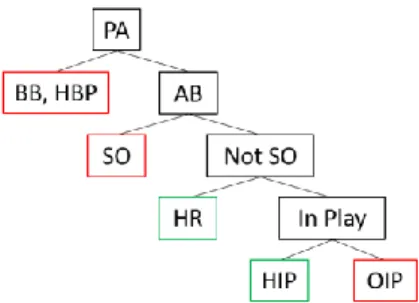
game proceeds with a player on the fielding team as the pitcher, throwing a ball which the player on the batting team tries to hit with a bat. When a player completes his turn batting, he gets credited with a plate appearance, which can have one of the following outcomes, as seen below:
Figure 1: Breakdown of a plate appearance.
Denotated in green are the events which result on a base hit and in red the events which are not. Thereafter, what this paper tries to achieve is to predict if a batter will achieve a Home Run (HR) or a Ball hit in play (HIP) among all his plate appearances (PA) during a game. In contrast it seeks to avoid Base on Balls (BB), Hit by Pitch (HBP), Strikeouts (SO) and Outs in Play (OIP). The most common approach which mostly resembles the model built in this project is forecasting the batting average (AVG). The main difference from both approaches is that the batting average does not account for Base on Balls (BB) and Hit by Pitches (HBP) scenarios.
There are many systems which predict offensive player performance including batting averages. These models range from simple to complex. Henry Druschel from Beyond the Boxscore identifies that the main systems in place are: Marcel, PECOTA, Steamer, and ZiPS (Druschel ,2016):
Marcel encompasses data from the last three seasons and gives extra weight to the most recent seasons. Then it shrinks a player’s prediction to the league average adjusted to the age using a regression towards the mean. The values used for this are usually arbitrary;
PECOTA uses data for each player using their past performances, with more recent years weighted more heavily. PECOTA then uses this baseline along with the player's body type, position, and age, to identify various comparison players. Using an algorithm resembling k-nearest neighbors, it identifies the closest player to the projected player and the closer this comparison is the more weight that comparison player's career carries.;
Steamer much like Marcel’s methodology uses a weighted average based on past performance. The main difference between the 2 is that Steamer’s the weight given for each year’s performance and how much it regresses to the mean is less arbitrary, i.e. these values vary between statistics and are defined by performing regression analysis of past players;
ZiPS like Marcel and Steamer uses a weighted regression analysis but specifically four years of data for experienced players and three years for newer players or players reaching the end of their careers. Then, like PECOTA, it pools players together based on similar characteristics to make the final predictions.;
Goodman and Frey (2013), developed a machine learning model to predict the batter most likely to get a hit each day. Their objective was to win the MLB Beat the Streak game, to do this they built a generalized linear model (GLM) based on every game since 1981. The variables used in the dataset, were mainly focused on the starting pitcher and batter performance, but also including some ballpark related features. The author’s normalize the selected features but no further pre processing was carried. The results on testing were 70% precision on correct picks and in a real-life test achieved a 14-game streak with a peak precision of 67,78%.
Clavelli and Gottsegen (2013), created a data mining model with the objective of maximizing the precision of hit predictions in baseball. The dataset built was scraped using python achieving over 35.000 samples. The features used in their paper regard batter and opposing pitcher’s recent performance and ballpark characteristics, much like the work the previous work analyzed. The compiled game from previous seasons were then inputed in a logistic regression, which achieved a 79,3% precision on its testing set. In the paper, it is also mentioned the use of a support vector machine, which ended up heavily overfitting resulting in a 63% precision in its testing set.
3 DATASET
The two main software used to develop this project were Microsoft Excel and Python. In the first stage, Microsoft Excel was used for data collection, data integration and variable transformation purposes. In a second stage, the dataset was imported to Python where the remaining data preparation, modelling and evaluation processes were carried out. In Python, the three crucial packages used were Pandas (dataset
structure and data preparation), Seaborn (data visualization) and Sklearn (for modelling and model evaluation). The elements used in the data collection and data storage processes are broadly depicted in Figure 2.
Figure 2: Data partitioning diagram.
The data considered for this project were the games played in Major League Baseball for the seasons 2015, 2016, 2017 and 2018. The features were collected from the three open source websites: Baseball Reference: Game-by-game player
statistics and weather conditions, which could be sub-divided into batting statistics, pitching statistics and team statistics (Baseball Reference, 2018);
ESPN: Ballpark factor (ESPN, 2018);
Baseball Savant: Statcast yearly player statistics, such as average launch angle, average exit velocity, etc (Baseball Savant, 2018).
In order to build the final dataset, the different features were saved in Excel Sheets. From Baseball Reference three sub sections were created: batter box-scores, pitcher box-scores and team box-scores. From Sports Savant batter yearly Statcast statistics. From ESPN the ballpark related aspects.
The chosen features categories will be explained for a general understanding on what they are and their potential importance for the models:
The Batter’s Performance category includes variables that look to describe characteristics, conditions or the performance of the batter. These variables translate into data features like the short/long term performance of the batter, tendencies that might prove beneficial to achieve base hits or even if the hand matchup, between the batter and pitcher, is favourable. The reason behind the creation of this category is that selecting good players based on their raw skills is a worthwhile advantage for the model.
Regarding the Batter’s Team Performance category, the only aspect that fits this category is the on-base percentage (OBP) relative to the team’s batter. Since baseball offense is constituted by a 9-player rotation if the batter’s team mates perform well, i.e. get on base, this leads to more opportunities for the batter and a consequently higher number of at-bats to get a base hit.
The Opponent’s Starting Pitcher category refers to the variables that regard the recent performance of the starting pitcher, from the opposing team of the batter being taken in consideration. These variables relate to the pitcher’s performance in the last 3 to 10 games and the number of games played by the starting pitcher. The logic behind the category is that the starting pitcher has a big impact on preventing base hits and the best pitchers tend to allow fewer base hits than weaker ones.
The Opponent’s Bullpen Performance category is quite similar to the previous one. Whereas the former category looks to understand the performance of the starting pitchers the latter focus on the performance of the bullpen, i.e. the remaining pitchers that might enter the game when starting pitcher get injured, get tired or enter to create tactical advantages. The reasoning for this category is the same as the previous one, a weaker bullpen tends to provide a higher change of base hits than a good one.
The Weather Forecast Category regards some weather conditions that have an impact on the target variable. The features that are taken into account are wind speed and temperature. Firstly, the temperature affects a baseball game in 3 main aspects: the baseball physical composition, the player’s reactions and movements, and the baseball’s flight distance (Koch & Panorska, 2013). If all other aspects remain constant higher temperatures lead to a higher chance of offensive production and thus base hits. Secondly, wind speed affects the trajectory of the baseball, which can lead to lower predictability of the ball’s movement and even the amount of time a baseball spends in the air (Chambers, Page & Zaidinis, 2003). Finally, the Ballpark Characteristics category englobes the ESPN ballpark hit factor, the roof type and the altitude. The “Park factor compares the rate of stats at home vs. the rate of stats on the road. A rate higher than 1.000 favours the hitters. Below favours the pitcher” meaning that this factor will have into consideration several aspects from this or other categories, indirectly (ESPN, 2018). Altitude is another aspect that is crucial to the ballpark, the higher the altitude the ballpark is situated the farther the baseball tends to travel. The previous statement is important to the Denver’s Coors Field, widely known
for its unusually high offensive production (Kraft & Skeeter, 1995).
Finally, the roof type of the ballpark affects some meteorological metrics, since a closed roof leads to no wind and a more stable temperature, humidity, etc when compared to ballparks with and open roof.
4 PRE-PROCESSING
The dataset built for this project is imbalanced, from which the total 155.521 samples, around 65,3% are batters that achieved at least a base hit and the remaining 34,7% are at batters whose game ended without achieving a base hit. Although not very accentuated it possible to determine that the dataset is imbalanced.
Table 1: Distribution of the dependent variable.
Hit Count Percentage
Yes 101.619 65,3%
No 53.902 34,7%
Total 155.521 100%
Both the under sample and oversample approaches were taken into consideration for the project. However, oversampling was not a feasible solution in the specific context of this paper, since the objective of the paper is to predict which are the best players for a given day and, therefore the creation of random games with random dates would disturb the analysis. This may have led to players having to play multiple fictitious games in the same days which would not make sense in the context of the regular season of baseball.
In conclusion the only method that will be tested for balancing the dataset is random under sampling. This consists on removing random observations from the majority class until the classes are balanced, i.e. have a similar number of observations for each of the dependent variable values.
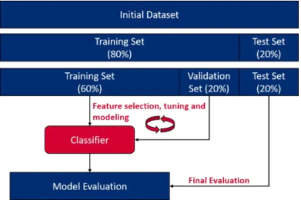
In this project it is implemented both holdout and cross-validation methods, since there was enough data. The initial dataset was firstly divided into training set (80%) and test set (20%) using a simple holdout method. Note that to achieve the best simulation possible, the division was done chronologically, i.e. the first 80% of the games correspond to the training set and the remainder to the test set.
Finally, for the training aspect of the project the training set was recursively divided into a smaller training set (60% of the total) and a validation set (20% of the total). This division implies that for
feature selection, hyper parameter tuning, evaluation the data was used with a stratified cross-validation technique with 10-folds. As seen below, figure 2 represents an overview of the partitions and their use for the project.
Figure 3: Data partitioning diagram.
Regarding normalization, the most common methods to obtain normalization of the variables is through normalization, standardization and scaling. The min-max normalization rescales variables in a range between 0 and 1, i.e. the biggest value per variable will assume the form of 1 and the lowest 0. It is an appropriate method for normalizing datasets where its variables assume different ranges and, at the same time, solves the mentioned problem of biased results for some specific algorithms that cannot manage variables with different ranges (Larose, 2005). This was the solution applied to normalize the numeric variables in the dataset:
𝑋∗= 𝑋 − min (𝑋) 𝑟𝑎𝑛𝑔𝑒(𝑋) =
𝑋 − min (𝑋)
max(𝑋) − min (𝑋) (1) In contrast, as some algorithms cannot cope with categorical variables, if it is intended the use of these types of variables in all models there is a need to transform these into a numerical form. Binary encoding was the solution implemented to solve this issue, where by creating new columns with binary values it is possible to translate categorical information into 1’s and 0’s (Larose, 2005).
Regarding missing values, only the Statcast variables (Average Launch Angle, Average Exit Velocity, Brls/PA% and Percentage Shift) had missing values, which comprised around 1% of all the features. These originated from the difference from the two data sources, i.e. some players were not in the Statcast database and therefore did not have a match when building the final database. To solve this issue the observations with missing values relative to Statcast features were deleted due to their immaterial size.
Figure 4: Top-down project diagram.
Additionally, some missing values were created after the variable transformation process. These missing values are the calculated performance statistics for the first game of every player in the dataset (pitcher or batter) and the same for every matchup pitcher vs batter. In sort, every observation which comprises the first game of a player its statistics from the previous “X games” will be NaN since its their first game in the dataset. These occurrences represented around 4% of the dataset for every batter and pitcher.
Finally, there were two main methods used to detect outliers in this project. In a first phase, it was calculated the z-score for all features with the objective of understanding what the variables with the most extreme values were considering the mean and standard deviation of the respective features. In this analysis values that are less than -3 standard deviations or greater than 3 standard deviations than the mean are usually considered outliers. In the context of our problem we cannot simply remove all observations with features that exceed these values but are a good start on understanding which variables have more outliers and their overall dimension in the context of the whole dataset (Larose, D., & Larose, C., 2014).
The other method used for outlier detection was boxplots, to visualize feature values in the context of their interquartile ranges. In this method any values that lie under the 1st quartile by more than 1,5 times the size of the interquartile range or over the 3rd quartile by more than 1,5 times the size of the interquartile range is considered an extreme value in
the context of the respective feature (Larose, D., & Larose, C., 2014).
In the end, the outlier detection of this project consisted on removing the most extreme values from feature using both the information from the z-score analysis and the visualization power of the box-plots. Note that due to the unknown influence of the outliers on the project, every model was tested with outliers and without the identified extreme values. With this it will be possible to have a good comparison of the performance of the models for both scenarios.
5 MODELLING
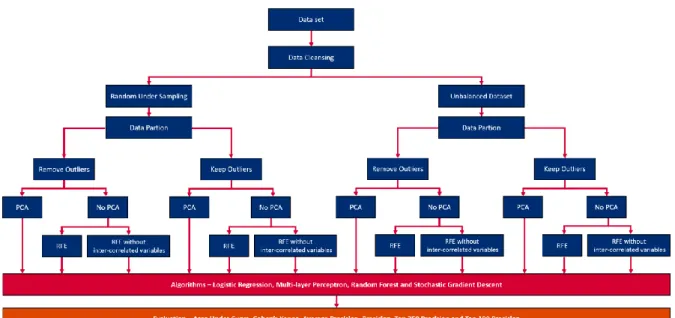
This chapter focus on presenting the methods used for modelling, feature selection and their respective hyper parameter tuning. Figure 4 depicts an end-to-end view of the paper, where it is possible to perceive the logic behind the processes performed to transform the initial dataset into insight on the problem in question.
Beginning in the dataset, various branching paths are created in order to test several hypotheses. This method enables the creation of the final 48 models, which are all evaluated equally and therefore provide a broader look on all the methods tested and what is the best final model for this problem.
In short, pre-processing and dimensionality reduction methods are applied to the initial dataset, as seen in figure 4. Thereafter the selected variables already pre-processed are used as inputs to the
algorithms, which output a probability estimate i.e. how likely is a batter to get a base hit in that game. Thereafter some evaluation metrics are applied to the models and the final conclusions are reached.
Over the course of this section a deeper look will be taken for the feature selection (PCA, no PCA, RFE and RFE without inter-correlated variables), the algorithms and the respective method used for hyper-parameter tuning and finally what evaluation metrics were applied to compare the final models created.
5.1 Algorithms
The logistic regression was developed by David Cox in 1958. This algorithm is an extension of the linear regression, which is mainly used in data mining for the modelling of regression problems. The former differs from the latter since it looks to solve classification problems by using a sigmoid function or similar to transform the problem into a binary constraint (Cox, 1958). The SAGA algorithm was chosen during the hyper parameter tuning for the logistic regression. SAGA follows the path of other algorithms like SAG, also present in the SKlearn library, as an incremental gradient algorithm with fast linear convergence rate. The additional value that SAGA provides is that it supports non-strongly convex problems directly, i.e. without much alterations it better adapts to these types of problems in comparison with other similar algorithms (Defazio, Bach & Lascoste-Julien, 2014).
A multi-layer perceptron is a type of neural network, inspired by the structure of the human brain. These algorithms make use of nodes or neurons which connect to one another in different levels with weights attributed to each connection. Additionally, some nodes receive extra information through bias values that are also connected with a certain weight (Zhang, Patuwo, & Hu, 1997).
The optimization algorithm used for training purposes was Adam, a stochastic gradient-based optimization method which works very well with big quantities of data and provides at the same time low computational drawbacks (Kingma & Ba, 2015). Regarding the activation functions, during the hyper parameter tuning the ones selected were ‘identity’- a no-op activation, which returns f(x) = x and ‘relu’- the rectified linear unit functions, which returns f(x) = max (0, x).
The concept of random forest is drawn from a collection of decision trees. Decision trees are a simple algorithm with data mining applications, where a tree shaped model progressively grows splitting into branches based on the information held
by the variables. Random forests are an ensemble of many of these decision trees, i.e. bootstrapping many decision trees achieves a better overall result, because decision trees are quite prone to overfitting the training data (Kam Ho, 1995).
The stochastic gradient descent is a common method for optimizing the training of several machine learning algorithms. As mentioned, it is used in both the multi-layer perceptron and logistic regression approach available in the SKlearn library. This away it is possible to use the gradient descent as the method of learning, where the loss, i.e. the way the error is calculator during training, is associated with another machine learning algorithm. This enables more control on the optimization and less computational drawbacks for the cost of a higher number of parameters (Scikit-learn, 2018a, Mei, Montanari & Nguyen, 2018).
During the parameter tuning, the loss function that was deemed most efficient was ‘log’ associated with the logistic regression. Therefore, for this algorithm the error used for training will resemble a normal logistic regression, already described previously.
5.2 Feature Selection
In data mining projects where there are high quantities of variables it is good practice to reduce the dimensionality of the dataset. Some of the reasons that make this process worthwhile are a reduction in computational processing time and, for some algorithms, overall better results. The latter results from the elimination of the curse of dimensionality – the problem caused by the exponential growth in volume related to adding several dimensions to the Euclidean space (Bellman, 1957). In conclusion, feature selection looks to eliminate variables with reductant information and keeping the ones who are most relevant to the model (Guyon & Elisseeff, 2003).
The first method used for selection the optimal set of variables was to use the recursive feature elimination (RFE) functionality in SKlearn. In a first instance, all variables are trained, and a coefficient is calculated for each variable, giving the function a value on which features are the best contributors for the model. Thereafter, the worst variable is removed from the set and the process is repeated iteratively until there are no variables left (Guyon, Weston, Barnhill & Vapnik, 2002).
Another method implemented for dimensionality reduction was the principal component analysis (PCA). This technique looks to explain the correlation structure of the features by using a smaller
set of linear combinations or components. By combining correlated variables, it is possible to use the predictive power of several variables in a reduced number of components.
Finally, the correlation between the independent features and the dependent variable were visualized as a tool to understand what the most relevant variables for the models might be. This analysis was carried for all variables, i.e. it was calculated the correlation between all dependent variables as well. This had the objective of doing a correlation-based feature selection, meaning that it is desirable to pick variables highly correlated with the dependent variable and the same time with low intercorrelation with the other independent features (Witten, Frank, & Hall, 2011).
5.3 Hyperparameter Tuning
The method chosen for hyperparameter tuning was Gridsearch with stratified 10-fold cross validation implemented using the SKlearn library. The process is similar to a brute force approach, where Python runs every possible combination of hyperparameters assigned and returns as the output the best combination for the predefined metrics (Scikit-learn, 2018b). This process was performed for every algorithm twice, once for the PCA and once for the no PCA formatted dataset. Needing to compare unbalanced and balanced datasets the metric chosen was area under curve.
5.4 Evaluation
The final step of the model process was to choose the metrics that better fitted the problem. The main constraints of the problem were to find good metrics that enabled the comparison between balanced and imbalanced datasets and, of course to achieve the objective of the project. The most appropriate metric to fulfil these requirements was precision with the objective of defining a tight threshold to secure a very high rate of correct predictions on players that would get a base hit. Nevertheless, other metrics that adapt to this type of problem were also calculated in order to get a better overall view of the final models, such as:
Area Under Curve; Cohen Kappa;
Precision and Average Precision.
Finally, for each model it was calculated the precision for the Top 250 and Top 100 instances, i.e. the instances with highest probability of being base hits as predicted by the models. This analysis
resembles the strategy that will be applied in the real world, for which only the top predictions will be chosen for the game. Note that this analysis will also give a very good impression on what threshold should be used for this point onward.
6 RESULTS
The objective of the paper was to create a model capable of consistently picking MLB players who will get a base hit on a given day. A dataset was built from scratch with variables that, according to the literature review, proved to have the most potential on predicting the aforementioned outcome.
During the process of developing the final 48 models, some alternatives were tested or pondered but later dropped. The main topics approached in such manner were:
Some sampling techniques;
Several machine learning algorithms did not reach the evaluation stage for various reasons;
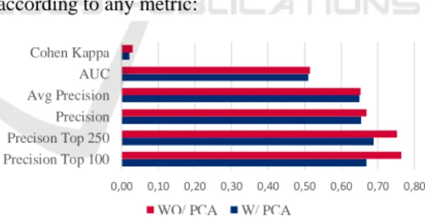
Several metrics were pondered but were dropped in detriment of the ones illustrated in this paper. The results of the final 48 models show some variance when all factors are considered, but overall it is viable to retain one main insight from the analysis on the test set metrics. As seen in the figure below, the use of PCA did not help the models perform better according to any metric:
Figure 5: Average model performance on test set, by use of PCA.
Apart from PCA, RFE and correlation-based feature selection were also used during the process of selecting the most valuable variables for the models. Comparing RFE results with the smaller subset of variables composed by the RFE selected variables minus the inter-correlated variables from those selections, it was possible to conclude that more often than not the smaller subset performs better than the full subset from the original RFE, thus highlighting some of the variables that are not so relevant when considered with the remaining selected variables. The most predominant variables being cut off, from this
0,00 0,10 0,20 0,30 0,40 0,50 0,60 0,70 0,80 Precision Top 100 Precison Top 250 Precision Avg Precision AUC Cohen Kappa
process, are batter and pitcher performance statistics and altitude. RFE selected several variables that belong to the same subcategory and hence are somewhat correlated. That way it was possible to withdraw some of these excess variables to achieve better overall results, leading to a belief that RFE alone was not the optimal strategy for feature selection for the dataset built for this project.
Regarding variable usage, the most used variables fall under the batter performance statistics category, additionally the models use at least one variable from each of the remaining categories, where the most prevalent are hits per innings for the starting pitcher (last 10 games), ESPN hit factor, temperature and hits per innings for the bullpen (last 3 games). The category with the least representation is the team batting statistics, as on-base-percentage (OBP) does not seem to add much prediction value on the outcome of the dependent variable.
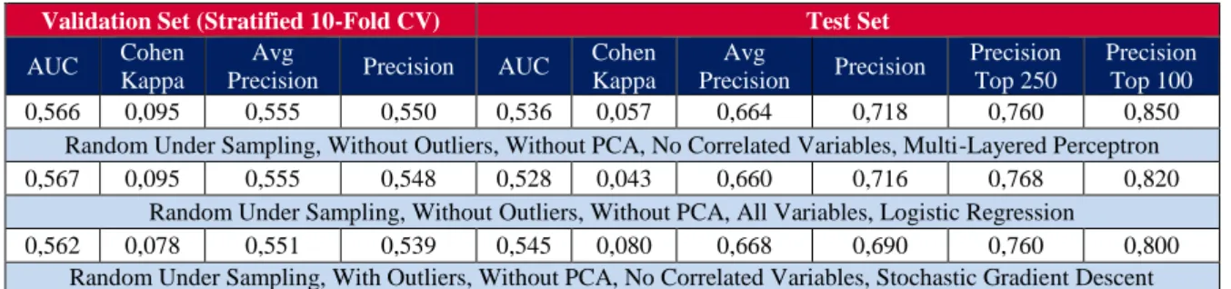
Considering the metrics chosen it was now possible to select the best models, table 2 presents the various metrics for the top 3 models selected. The logic behind the selection was to choose the models with the highest precision on the Top 100 and 250 instances, giving most attention to those that also performed well on other metrics.
All in all, balanced datasets work well on this project and, most of the top performing models came from sets with random under sampling. When analysing balanced datasets, these outperform the unbalanced datasets in every metric except for the top 100 and 250 precision, deeming most of them irrelevant. Additionally, imbalanced datasets also had the inconvenience of choosing the most common label for most instances, during validation, producing ambiguous results and limiting possible analysis and conclusions between these results.
Furthermore, methods like outlier’s removal, inter-correlated variable removal and the choice of algorithm do not appear to produce dominant strategies in this project and in the right conditions all possibilities produce good results, as seen in the diversity of methods used in the top 3 models.
In a real-life situation, the 1st model in the tables above would provide the best odds of beating the streak with an expected rate of correct picks of 85%, in situations where the model’s probability estimate is very high. The remaining top models also prove to be viable, in which models with precision on Top 250 instances higher than the former model give a slight improvement on expected correct picks at lower probability estimations.
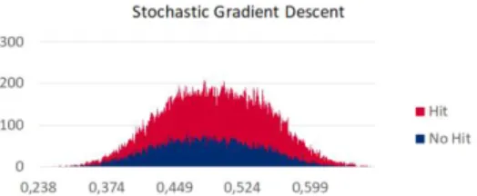
The information used to rank the instances by probabilities estimates was further used to calculate at what threshold can we expect to achieve similar correct picks. Note that it is not mandatory to pick a player every single day, therefore it is optimal to wait and pick only when the models are confident enough on when a base hit is occurring. For this analysis figures 4 to 6 explore the hits and no hits per probability estimate of each of the top 5 models:
Figure 6: Distribution of probability estimates for the best Multi-Layered Perceptron.
Figure 7: Distribution of probability estimates for the best Logistic Regression.
It possible to note a sweet spot in the far right of each of the figures, where there are areas with no or very few no-hit instances where the models predict hit. After a thorough analysis it is impossible to
Table 2: Distribution of the dependent variable.
Validation Set (Stratified 10-Fold CV) Test Set
AUC Cohen Kappa
Avg
Precision Precision AUC
Cohen Kappa Avg Precision Precision Precision Top 250 Precision Top 100 0,566 0,095 0,555 0,550 0,536 0,057 0,664 0,718 0,760 0,850
Random Under Sampling, Without Outliers, Without PCA, No Correlated Variables, Multi-Layered Perceptron
0,567 0,095 0,555 0,548 0,528 0,043 0,660 0,716 0,768 0,820
Random Under Sampling, Without Outliers, Without PCA, All Variables, Logistic Regression
0,562 0,078 0,551 0,539 0,545 0,080 0,668 0,690 0,760 0,800
choose a threshold that gives an 100% change of only picking hit instances that were correctly predicted, for 57 instances. Nevertheless, the top 100 strategy still works well in this analysis and, in table 15, it is depicted the different values that are good thresholds to achieve above 80% expected correct picks.
Figure 8: Distribution of probability estimates for the best Stochastic Gradient Descent.
Table 3: Threshold analysis on top 3 models.
The models provide different ranges of probabilities but in the end all thresholds fall under approximately 80%-90% of the overall distributions, according to the z-score. Some ensembles techniques were tried to improve the expected results, such as majority voting and boosting techniques but none of these techniques provided any improvement in the results and were later dropped.
Table 4: Project results versus results of other strategies.
The most basic strategies used for playing a game like Beat the Streak is to either pick a complete random player or to pick one of the best batters in the league. These strategies, as expected, have very low results compared to any of the models. From the models identified during the literature review, it is possible to see improvements and strategies that give a player an advantage over the simple strategies. The best and preferred method used by other papers is to use a type of linear model, that was also tried during this project. Nevertheless, the multi-layer perceptron, mentioned in the top 3 algorithms, provides a 5-percentage point improvement over the best model from other papers. The improvements over the
previous works, mentioned in Figure 4 and previously discussed in the end of section 2 of this paper, cannot be attributed to a single factor. However, the main differences that, in the end, resulted in a better outcome of this paper, comparatively to the other two, are as follow.
A wider scope of variable types. In other works, the authors focus primarily on the use of variables regarding the batter’s and pitcher’s performance, as well as ballpark characteristics. In this paper the focus shifts to the use to a wider range of variable types, which in the end proved to be important to provide a wider understanding on the event being predicted.
The experimentation of several pre-processing methods, modelling methods and algorithms. In this paper no method is deemed to be definitive and by creating a greater number of models it was possible to test several methods and test combinations of those in order to get a better understanding on what are the processes that work and, with this, be more confident that it was possible to arrive to a good conclusion. This contrasts with the the more unilinear direction followed by the other authors who tended not to experiment several approaches to their problem.
Finally, the overall strategy of evaluation of this paper better suits the task being presented. In the papers mentioned the authors focus on standard metrics to evaluate the results of the models, such as precision. However, because of the nature of the game Beat the Streak, it is not crucial to evaluate all features in the test set, but more importantly we are to be sure of the picks being made. Therefore, by wielding the probability estimates in conjunction with the 100 or 250 precision metrics, one can achieve more accurate conclusions.
7 CONCLUSIONS
The main objectives of this project were to produce a model that could predict which players were most likely to get a base hit on a given day and, in this sense, provide an estimation of the probability of said event occurring, for the use of stake holders in MLB teams.
To achieve these objectives the following steps were taken:
Build a database using open-source data including features from a variety of categories;
Use descriptive statistics and data visualization techniques to explore the value of the features identified during the literature review;
Build a predictive model using data mining and machine learning techniques, which predicts the
Probability Estimates MLP LG1 SGD
Maximum probability 0,658 0,671 0,679 Minimun probabilty 0,242 0,218 0,238
Threshold top 100 0,608 0,616 0,643
Z-score threshold 0,880 0,878 0,918
Expected correct ratio 85% 82% 80%
Paper
Random guessing Picking best player
Algorithm Linear Model MLP
Goodman & Frey (2013) 70%
-Clavelli & Gottsegen (2013) 80%
-Best Models (this paper) 82% 85%
Expected Correct Picks ≈ 60% ≈ 67%
probability of a base hit occurring for each instance;
Apply the model on a test set and analyse the predictions to select the best models and to find the optimal thresholds.
Firstly, the data needed for this project was collected from Baseball Reference, Baseball Savant and ESPN websites. This data was distributed into different Microsoft Excel sheets and later integrated into a single database, displaying the features from each batter’s game, not including pitchers batting.:
Secondly, the database was imported to Python and structured using the Pandas library. Several descriptive statistics and data visualization techniques were applied to the database, using the Seaborn package to extract insights on the quality of the data, to understand what type of transformations were needed and to gain insights on some the variables being used. Throughout the latter process it was possible to find out that the best variables in terms of correlation to the dependent feature were mostly batting statistics. At the same the time, variables from this sub-category suffered from inter-correlation with one another, which was taken into consideration during the feature selection.
Using the insights gained from the second step it was possible to do the pre-processing and transformations on the dataset, making it ready for the third step of the project. Thereafter, several models were built with the main constraints being data set balancing, the use of outliers, the use of PCA and a feature selection using RFE or using RFE in conjunction with a correlation-based feature selection creating a smaller subset of features from the RFE selected variables.
From the final 48 models created it was possible to retain some insights:
PCA did not perform as well as the other forms of feature selection;
Overall, balancing the datasets using random under sampling obtained better results than no balancing;
It was possible to obtain simpler models by removing inter-correlated variables from the RFE selected features and obtain similar or better models.
Finally, after analysing the performance of the models against the test set, the top 3 models were chosen as possible candidates for usage in a real-world situation. With the ability to calculate the probability estimates for each instance, it was possible to then find the thresholds for each model. The best model gave an expected correct pick rate of
85% on the top 100 picks (precision on top 100 most probable instances), on test set, i.e. half a season worth of instances.
The model that provides these results is a multi-layer perceptron, no outliers, no PCA and with the removal of inter-correlated variables from the original feature selection. When compared to similar works, this model has about 20 percentage points gain on precision over the best basic strategy and a 5 percentage points gain over the best model analyzed during the literature review.
Nevertheless, a base hit in baseball has a very close relationship to a player’s ability and other factors already mentioned during this paper. These types of events are prone to be random, since there are a lot of elements that are hard to quantify into features and, thus cannot be fully translated in a machine learning model. The influence of luck can be diminished but it is hard to ever obtain a 100% model in predicting these events. The project at hand had some good results but it is unlikely that with an 85% expected correct pick ratio, it will predict correctly 57 times in a row.
The main points for improvement for this project would be:
Collect data from more seasons;
Experiment with a wider variety of sampling techniques;
Identify new variables, especially from factors not used in this project, for example defensive performance from the opposing team;
Experiment with other algorithms and further tune the hyperparameters used in them;
Effective use of some form of ensemble technique.
REFERENCES
Alamar, B., 2013, Sports Analytics: A Guide for Coaches,
Managers, and Other Decision Makers. Columbia
University Press.
Baseball Reference, 2018, Baseball Reference. Retrieved
from Baseball Reference:
https://www.baseball-reference.com
Baseball Savant, 2018, Baseball Savant. Retrieved from Baseball Savant: https://baseballsavant.mlb.com Beat the Streak, 2018, Beat the Streak: Official Rules.
Retrieved from Beat the Streak: http://mlb.mlb.com/ mlb/fantasy/bts/y2018/?content=rules
Bellman, R., 1957, Dynamic programming. Princeton, NJ: Princeton University Press.
Chambers, F., Page, B., & Zaidinjs, C., 2003, Atmosphere, weather and baseball: How much farther do baseballs
really fly at Denver’s Coors Field. Prof. Geogr. 55th
edition, 491-504.
Clavelli, J., & Gottsegen, J., 2013, Maximizing Precision of Hit Predictions in Baseball.
Collignon, H., & Sultan, N., 2014, Winning in the Business
of Sports. ATKearney.
Cox, D., 1958, The Regression Analysis of Binary Sequences. Journal of the Royal Statistical Society.
Series B, 20(2), 215-242.
Defazio, A., Bach, F., & Lacoste-Julien, S., 2014, SAGA: A Fast-Incremental Gradient Method with Support for
Non-Strongly Convex Composite Objectives.
Advances in Neural Information Processing Systems,
27, pp. 1-9.
Druschel, H., 2016, Guide to the Projection Systems.
Retrieved from Beyond the Box Score:
https://www.beyondtheboxscore.com/2016/2/22/1107 9186/projections-marcel-pecota-zips-steamer explained-guide-math-is-fun
ESPN., 2018, ESPN Hit Factor. Retrieved from ESPN: http://www.espn.com/mlb/stats/parkfactor
Goodman, I., & Frey, E., 2013, Beating the Streak: Predicting the MLB Players Most Likely to Get a Hit each Day.
Guyon, I., & Elisseeff, A., 2003, An Introduction to Variable and Feature Selection. Journal of Machine
Learning Research, 3, 1157-1182.
Guyon, I., Weston, W., Barnhill, S., & Vapnik, V.2002, Gene Selection for Cancer Classification using Support Vector Machines. Machine Learning, 46(1-3), 1-3. Jia, R., Wong, C., & Zeng, D., 2013, Predicting the Major
League Baseball Season.
Kam Ho, T., 1995, Random Decision Trees. Proceedings.
3rd International Conference on Document Analysis and Recognition, (pp. 278-282).
Kingma, D., & Ba, J., 2015, Adam: A Method for Stochastic Optimization. 3rd International Conference
for Learning Representations, (pp. 1-15).
Koch, B., & Panorska, A., 2013, The Impact of Temperature on major League Baseball. Weather,
Climate, and Society journal, 5(4), 359-366.
Kraft, M., & Skeeter, B., 1995, The effect of meteorological conditions on fly ball distances in north American Major League Baseball games. Geogr. Bull, 37, 40-48. Larose, D., & Larose, C., 2014, Discovering Knowledge in
Data: An Introduction to Data Mining (2 ed.). John
Wiley & Sons, Inc.
Larose, D., 2005, Discovering Knowledge in Data: An
Introduction to Data Mining. John Wiley & Sons, Inc.
Mann, R., 2018, The Marriage of Sports Betting, Analytics and Novice Bettors.
Mei, S., Montanari, A., & Nguyen, P., 2018, A Mean View
of the Landscape of Two-Layers Neural Networks.
1-103.
MLB., 2018, Glossary / Statcast. Retrieved from MLB: http://m.mlb.com/glossary/statcast
Mordor Intelligence, 2018, 2018 Sports Analytics Market - Segmented by End User (Team, Individual), Solution (Social Media Analysis, Business Analysis, Player
Fitness Analysis), and Region - Growth, Trends and Forecast (2018 - 2023).
Ockerman, S., & Nabity, M., 2014, Predicting the Cy Young Award Winner. PURE Insights, 3(1), 9.
Scikit-Learn, 2018a, Stochastic Gradient Descent.
Retrieved from: https://scikit-learn.org/stable/modules/ sgd.html#classification0
Scikit-Learn, 2018b, Grid Search CV. Retrieved from: https://scikitlearn.org/stable/modules/generated/sklear n.model_selection.GridSearchCV.html#sklearn.model _selection.GridSearchCV
Stekler, H., Sendor, D., & Verlander, R., 2010, Issues in
sports forecasting. International Journal of
Forecasting, 26(3), 606-621.
Valero, C., 2016, Predicting Win-Loss outcomes in MLB regular season games – A comparative study using data mining methods. International Journal of Computer
Science in Sport, 15(2), 91-112.
Witten, I., Frank, E., & Hall, M., 2011, Data Mining:
Practical Machine Learning Tools and Techniques (2 ed.). Morgan Kaufmanne, Inc.
Wolf, G., 2015, The Sabermetric Revolution: Assessing the Growth of Analytics in Baseball by Benjamin Baumer and Andrew Zimbalist (review). Journal of Sport
History, 42(2), 239-241.
Zhang, G., Patuwo, B., & Hu, M., 1997, Forecasting with artificial Neural Networks: The state of state of the art.