On the application of Structural Credit
Risk models to Sovereign issuers
Dissertation by
Guilherme Donário Miranda
Student Number: 152416016
Dissertation written under the supervision of
Professor Nuno Silva
Dissertation submitted in partial fulfilment of requirements for the MSc in Finance, at the Universidade Católica Portuguesa.
ABSTRACT
Title: On the Application of Structural Credit Risk models to Sovereign issuers. Author: Guilherme Donário Miranda
Keywords: Credit Default Swaps, probability of default, Portuguese Sovereign, geometric
Brownian motion, risk neutral, physical measure
This dissertation uses CDS spreads to extract the probability of default of the Portuguese sovereign using a structural credit risk model. The model considered assumes that the government revenue follows a geometric Brownian motion. In addition, the government is assumed to have fixed costs corresponding to its total expenditure. The sovereign defaults at the first time its revenue falls below a certain level, which is estimated in this thesis as a multiple of the government debt. Under the assumption of a 40% recovery rate, estimates on the 5-year probability of default were extracted. This was done both under the risk neutral and the physical measure. This was possible assuming that the market price of risk implicit in sovereign CDS markets was equal to the one implied in Portuguese listed equities.
The results obtained were in line with expectations. The probability of default of the Portuguese government is close to zero in 2007, 2008, 2016 and 2017 and reaches very high levels in 2011 and 2012. Though the highest probability of default (under both measures) is observed in 2011, the largest difference between the probability of default under the risk neutral and physical measures is observed in 2012. In this year, the difference in the 5-year probability of default under the two measures reaches 13.90 percentage points.
SUMÁRIO
Título: Aplicação de modelos Estruturais de Risco de Crédito a Soberanos emissores Autor: Guilherme Donário Miranda
Palavras-chave: Credit Default Swaps, probabilidade de incumprimento, Estado Português,
movimento Browniano geométrico, medida neutra, medida física.
Esta tese utiliza spreads dos CDS para extrair a probabilidade de incumprimento do Estado Português utilizando um modelo estrutural de risco de crédito. O modelo considerado assume que a receita do governo segue um movimento Browniano geométrico. Para além disso, assume-se que o governo tem custos fixos correspondentes à sua despesa total. O soberano entra em incumprimento quando a sua receita desce abaixo de um determinado nível que, nesta tese, é estimado como um múltiplo da dívida soberana. Assumindo uma taxa de recuperação de 40%, a probabilidade de incumprimento a 5 anos foi extraída na medida neutra ao risco e a física. Isto foi possível assumindo que o preço de mercado do risco implícito nos CDS dos soberanos era igual ao implícito em empresas Portuguesas cotadas em bolsa.
Os resultados obtidos estão em linha com os esperados. A probabilidade de incumprimento do estado Português a 5 anos foi próxima de zero nos anos de 2007, 2008, 2016 e 2017 e atingiu níveis extremamente elevados em 2011 e 2012. O valor mais elevado para esta variável, em ambas as medidas, foi observado em 2011. A maior diferença entre a medida neutra ao risco e a medida física ocorreu em 2012. Neste ano, a diferença na probabilidade de incumprimento a 5 anos entre as duas medidas atingiu 13.90 pontos percentuais.
ACKNOWLEDGEMENTS
First and foremost, I would like to thank my family, specially my parents and my brother, for their support throughout my academic studies. They have always given me crucial advices on critical times and backed up my decisions. Only due to their encouragement did I handle to finish my studies with such results.
I am also very grateful to my supervisor Nuno Silva, who has provided me guidance and prompt feedback along my dissertation period. His knowledge, encouragement and patience were thus fundamental for the completion of my thesis.
Another special thank you note goes to my friend André Baptista for his endless coding lessons. Without him it would be extremely harder to accomplish the results I was able to.
I would also like to express my appreciation to my girlfriend, Sofia, for giving me encouragement and support throughout all the writing of this thesis.
Finally, my gratitude also go to my colleagues and friends who have understood the effort required to write the dissertation and that tried to help and encourage when I needed them.
TABLE OF CONTENTS ABSTRACT ... II SUMÁRIO ... III ACKNOWLEDGEMENTS ... IV TABLE OF CONTENTS ... V TABLE OF FIGURES ... VI TABLE OF TABLES ... VII GLOSSARY ... VIII
CHAPTER 1: INTRODUCTION ... 1
CHAPTER 2: LITERATURE REVIEW ... 3
CHAPTER 3: THE MODEL ... 8
CHAPTER 4: DATASET ... 13
CHAPTER 5: MODEL ESTIMATION ... 18
CHAPTER 6: RESULTS ... 21 CHAPTER 7: CONCLUSIONS ... 28 CHAPTER 8: REFERENCES ... I CHAPTER 9: APPENDIX ... IV APPENDIX 1 ... IV APPENDIX 2 ... VI APPENDIX 3 ... VIII APPENDIX 4 ... IX APPENDIX 5 ... X
TABLE OF FIGURES
Figure 1 - Portuguese revenue. ... 14
Figure 2 - Portuguese expenditure. ... 14
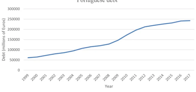
Figure 3 - Portuguese debt. ... 15
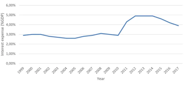
Figure 4 - Portuguese interest expense. ... 16
Figure 5 - MPDR average for the Portuguese firms. ... 23
Figure 6 – 5-year Probabilities of Default of the Portuguese Sovereign. ... 26
Figure 7 - Difference between PDs. ... 27
TABLE OF TABLES
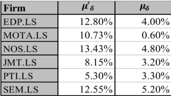
Table 1 - μδ for the Portuguese firms. ... 22
Table 2 - MPDR for the Portuguese firms. ... 23
Table 3 - Sigma for the Portuguese sovereign. ... 24
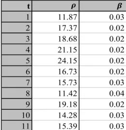
Table 4 - Rho and Beta for the Portuguese sovereign. ... 24
GLOSSARY
BLUE - Best Linear Unbiased Estimators BP test - Breusch–Pagan test
BSM - Black-Scholes-Merton model CCA - Contingent Claim Analysis CDS - Credit Default Swap
CFI - Investing Cash flow CFO - Operational Cash Flow CRA - Credit Rating Agencies
CUSP - Credit Underlying Securities Pricing EBIT - Earnings before Interest and Taxes EDF - Expected Default Frequency
EU - European Union
FCFE - Free Cash Flow to Equity FPT - First-Passage-Time model GBM - Geometric Brownian Motion IMF - International Monetary Fund LGD - Loss Given Default
MLE - Maximum Likelihood Estimator MM - Mixed Maximization
MPDR - Market Price of Diffusion Risk NFC - Non-Financial Corporations PD - Probability of Default
CHAPTER 1: INTRODUCTION
Credit risk - the risk that a borrower may not honour a debt commitment - is a central topic for financial institutions and financial economists. Several approaches have been developed through time. Among the most well-known are multivariate discriminant analysis, Altman Z-scores linear probability models, logit and probit models, intensity based reduced form models and structural models. The latter employ modern option pricing theory to price contingent claims. Structural models allow, in one setting, to link fundamental characteristics of debt issuers, notably the value of their assets, nominal liabilities and the business risk, with their Probabilities of Default (PDs) and Loss Given Defaults (LGDs). Several studies have shown that, when properly calibrated to quoted firms, structural credit risk models can outperform more traditional models which are based on accounting information to predict default. This superior performance is justified by the use of financial assets prices, which incorporate agents’ expectations (Calin & Popovici, 2014).
The majority of structural credit risk models were developed having in mind non-financial corporations (NFC). Though possible, credit risk models’ application to sovereigns is challenging. Firstly, it is conceptually difficult to define what the assets of sovereigns are. One possibility is to consider that the government asset corresponds to the present value of all future revenues, though it is the sovereign itself that sets tax rates, the recent crisis has shown that there are limits to tax rates and this can derive from the sovereigns’ will or the non-capacity of charging the necessary taxes to pay back debt. Second, opposing to what happens to firms, sovereigns do not have limited liability. Third, model calibration is harder in the case of sovereigns. While firms have several financial assets that are traded - such as stocks, bonds, Credit Default Swap (CDS) and options -, sovereigns only have bonds and CDS. Finally, sovereigns differ from firms regarding default procedures and law enforcement. The case of Argentina is tantamount of this.
Even though applying structural credit risk models to sovereigns is more complex than to the private sector, several authors have used different methods to do so. Most of the progress in this field came from the industry and policy makers rather than from the academia. The International Monetary Fund (IMF) has issued several papers on the application of structural models to monitor sovereigns’ credit risk. This is the case of Gapen et al., 2008. Most of these papers
focus on emerging markets, where the government has controlling powers over the central bank policy. Notice that in case the sovereign controls the Central Bank, the latter can always be forced - by the government - to issue money, risking its long-term inflation goals but avoiding default. In this case, sovereign’s credit in the country’s currency is generally seen as being almost negligible. For certain, this is not the case in the Euro area. Following the sovereign debt crisis, Credit Suisse extended its structural model known as CUSP (Credit Underlying Securities Pricing) to sovereigns. From the academia side, Jeanneret (2012) developed a endogenous barrier structural credit risk model suitable for euro area sovereigns.
The goal of this dissertation is to contribute to the literature on the application of structural credit risk models to sovereigns. This thesis applies a modified version of the static version of the Goldstein, Ju, & Leland (2001) model to estimate the probability of default risk of the Portuguese Sovereign. In this modified version, the state variable is the government’s revenue (instead of the firms’ Earnings before Interest and Taxes (EBIT)) and the firms’ interest expense is replaced by total government expenditure. The sovereign defaults at the first time its revenue falls below a certain level, which is estimated in this thesis as a multiple of the government debt. Under the assumption of a 40% recovery rate, estimates on the 5-year probability of default were extracted. This was done both under the risk neutral and the physical measure. The latter was only possible because it was assumed that the market price of risk implicit in sovereign CDS markets was equal to the one implied in Portuguese listed equities. The market price of risk implicit in Portuguese equities was estimated also using a structural model. This dissertation is divided into 6 more chapters. Chapter 2 is the literature review, Chapter 3 presents the model. Chapters 4 and 5 describe the used dataset and the model’s estimation, respectively. Chapter 6 presents the results for the Portuguese case for the period between 2001 and 2016. Lastly, Chapter 7 concludes.
CHAPTER 2: LITERATURE REVIEW
Structural Credit Risk models started with Black & Scholes (1973) and Merton (1974) seminal papers. In the Black-Scholes-Merton model (BSM) the case of a firm financed by equity and a pure discount bond with a certain maturity, whose market value of assets follow a geometric Brownian motion (GBM), is considered. At the debt maturity, the firm is liquidated with one of two possible sceneries occurring. One alternative is that if the firm’s asset value surpasses the promised payments 𝐵, the lenders receive the promised amount and the residual value of the assets is given to the shareholders. However, the second alternative considers that, if the value of the firm’s assets is lower than the promised payments 𝐵, the firm enters into default and the lenders receive a payment equal to the value of the assets, leaving the shareholders without any payment. Based on this, Black-Scholes-Merton concluded that creditors are basically shorting a put option1 on the assets of the borrowing firm, in which the strike price is
equal to the face value of debt (𝐵). Using the put-call parity relationship, it is possible to reach to the conclusion that equity is a call option on the firm’s assets, in which the strike price is equal to the book value of the firm’s liabilities, i.e. the value of the promised payments. From the put option, which can be interpreted as the expected loss of the debt, one can take the model credit spread, which can be shown to be a function of the maturity of debt, the leverage (𝐵) and the business risk of the assets of the firm (𝜎2).
The BSM model makes several assumptions, which several authors have tried to relax over the time. As an example of that, Black & Cox (1976) dropped the assumption which states that the default time of a bond has to be at its maturity. In their model, the firm defaults when the asset value reaches, for the first time, a downward barrier exogenously defined. This means that, the model is treated as a first-passage-time model (FPT). Black & Cox (1976) had, as a motivation for the development of the model, the need to take into account the existence of bond covenants. Following the last section in Black & Cox (1976) paper, Leland (1994) came up with a framework in which a firm’s optimal default threshold is endogenous. In this model, the decision of default is assumed to be made by managers, whose actions try to maximize the equity value across time. Therefore, in the endogenous default model, the default barrier is such that the value of the firm’s equity is maximized through the smooth pasting condition. In addition to that, in the referred Leland (1994) model, debt is considered to be perpetual.
Leland & Toft (1996) introduced an additional concept to Leland's (1994) model – the rollover. In their model, a firm has to constantly rollover its maturing debt by issuing new debt with the same maturity and face value at market price. Also, equity holders are the ones who bear the loss/gain of this rollover. They show that whenever rollover is more frequent, shareholders choose to default earlier which is due to the debt repricing. If credit risk rises, and debt needs to be rolled over, it may have to be refinanced at a higher rate and more interest has to be paid in the future. The opposite occurs when credit risk falls since the relation is not linear. This means that, when it falls, it leads to an increase in the optional default barrier.
All the aforementioned models assume constant risk-free rates. Opposing to those, Longstaff & Schwartz (1995) wrote one of the first articles that considered stochastic interest rates. In their paper, the risk-free interest rate dynamics are given by the Vasicek (1977) model.
The poor performance these models presented (Eom, Helwege, & Huang, 2004), mainly regarding short term spreads, has motivated Zhou (2001) to propose that the value of the asset follows the jump-diffusion process. The two main parts of every jump-diffusion model are the Brownian motion (diffusion part) and the Poisson process (jump part), under which a firm can enter into default instantaneously due to a sudden drop in its value. In the case of Zhou (2001), the jumps are taken from a normal distribution.
One of the main issues regarding the structural framework is the fact that, though there are non-observable key variables in the model, these are intrinsically assumed to be non-observable. The value of assets, as well as their volatility, need to be estimated. Adding to this, several models consider the existence of default costs, which depending on the model may affect equity or only debt prices. Furthermore, unless one assumes some number based on empirical studies on bankruptcy costs, this also has to be estimated.
In the case of Merton’s model, in order to solve this issue, four main approaches have been proposed. The first one, proposed by Jones, Mason, & Rosenfeld (1984) and Ronn & Verma (1986), consists on applying the Itô’s lemma to the equity function. Using either option implied volatilities or historical volatilities to proxy for equity return volatility, this leads to a system with two equations and two variables. Secondly, Vassalou & Xing (2004) applied an iterative method to estimate the unknown variables (KMV method). A third approach, by Duan (1994) and Duan (2000), estimated the unknown variables using the transformed-data maximum
likelihood method (MLE). This estimation method consists of, in a simplified way, finding a certain parameter 𝜃 that is most probable to have generated the data 𝑋. Despite not being optimal in the minimum variance sense, the ML estimator is unbiased. Therefore, the idea behind these authors’ study is to use observed prices of a derivative contract to compute maximum likelihood parameters’ estimates for an unobserved asset value process. Finally, the model developed by Brockman & Turtle (2003) and Eom et al. (2004) consists on using the market value of equity and the total nominal debt to obtain a proxy for the market value of assets. Though, this option was heavily criticized by Wang & Li (2004), whom were able to show, using Monte Carlo simulations, that the approach used by Eom et al. (2004) could lead to biased predictions, as well as not being consistent with the option pricing theory barrier conditions.
Opposing to the issues identified by many authors, Wang & Li (2004) and Duan, Gauthier, & Simonato (2004) were capable of demonstrating that the transformed data approach is the most accurate one to estimate the unknown variables.
Moreover, Forte (2011) and Santiago Forte & Lovreta (2012) tried different ways of calibrating the parameters. They concluded that using the mixed maximization (MM) algorithm (proposed by Forte (2011)) for estimating the CDS price is the one that obtains fewer errors when compared to other methods, thus being the best numerical method.
All articles mentioned above had a focus point on either corporate securities pricing, corporate credit risk or corporate finance issues. Though, none of those studies have referred applications to sovereign credit risk as the application of structural models to sovereigns is still an emerging field. In fact, most of the work developed in the sovereigns’ field came from the industry, rather than from academia.
Initial work on this topic came, as stated above, from the academia, and started by considering a country’s willingness to repay its external debt to be a random variable following a stochastic process, in a work developed by Chesney & Morisset (1992). These authors considered that a default occurs when a country’s willingness to pay is lower than the face value of the external debt, at time 𝑇 (maturity time). This idea was then further developed by Claessens & Pennacchi (1996), who assumed this could be translated into a risk indicator that also follows a stochastic process. From their study it can be observed that default would occur when that risk indicator fell below zero.
In another well-known study, from Gray et al. (2007), it is considered that the assets side is composed by FX reserves, net fiscal assets and public assets. In the liabilities side, one could find guarantees, foreign and local-currency debt and base money. Furthermore, these authors also considered the foreign-currency to be the senior claim and the local-currency debt plus base money the junior claim, i.e. equity.
Furthermore, Jeanneret (2013) applied structural credit risk modelling (with endogenous default barrier) to European countries. This paper represented a new framework to analyse the creditworthiness of a country, by providing a closed-form solution for the computation of the Credit Spreads. In his paper, Jeanneret (2013) concluded that the daily variation of sovereigns credit spreads depends mainly on model-implied spreads, using specific information in the daily stock markets.
Another important application of the previous work was made by Lee, Shih, & Wang (2015) who investigated a country’s credit risk by using a barrier option pricing model, which they applied to 15 countries. In their paper, the authors started by using the same approach as Gray et al. (2007) – the sovereign balance sheet - and further constructed a barrier model, using the transformed-data MLE approach to calibrate the unknown parameters.
Moving from what has been studied by the academia to the industry side, a first advance that can be mentioned is related to the application of CCA to sovereign. This has gained strength following a series of articles produced by IMF - for instance, Gapen et al. (2008).
Adding to that, Credit Suisse developed a credit model to be applied to sovereigns. Being a forward-looking model for credit spread risks, it uses market implied volatility information to derive measures of spread risk. From all the components of CDS spreads2, Credit Suisse
believes that the mark-to-market component is the one playing a major role in evaluating CDS as an asset class, mainly in the sovereign CDS spreads. Summing up, CUSP assesses mark-to-market risk in a systematic and forward-looking way. In their CUSP model (Martin et al., 2007), Credit Suisse uses as input the CDS curve (level and slope), the leverage and the equity option-implied volatility. One of the main strengths of this model is that it is not calibrated to
2 Credit spreads can be decomposed into the following components: Expected loss, uncertainty, liquidity risk and
historical time series. Indeed, instead of that, only the latest market observations are used to estimate the parameters of the model.
KMV is a leading provider of credit risk analysis tools, which was acquired by Moody’s in 2002. After such acquisition, Moody’s further pioneered the application of modern financial theory to improve the progress made by the industry for assessing credit risk for sovereigns. As a result of that, Moody’s KMV model is another important example to be analysed.
Not all of its features are publicly available. From what is known, this model assumes that the boundary depends on the maturity structure of the debt instruments issued by the obligor. It estimates the asset value and asset volatility of the borrowing firm. Despite this method being firm-specific, the key features used by the KMV model can be extended and hence be applied to compute the credit risk of sovereign bonds issued by countries.
The KMV model is based on the structural approach to calculate the Expected Default Frequency (EDF). Those are estimates of corporate borrowable one-year default rates and, as such, are the exact counterparts of the one-year probability of defaults implied by academic models.
One drawback that can be found regarding KMV model is the short time span of the probabilities of default, which limit significantly the scope of their evaluation. Nevertheless, by being based on a particularly rich proprietary dataset, the PDs provide an additional perspective on the implications of the academic models. Curiously, the probabilities of default obtained using the Moody’s KMV model are found to be the highest across other models, thus, over-predicting risk.
CHAPTER 3: THE MODEL
Assume that the government revenue follows a GBM, whose dynamics are given under measure P3 by 𝑑𝛿𝑔𝑜𝑣 𝛿𝑔𝑜𝑣 = 𝜇𝑔𝑜𝑣𝑑𝑡 + 𝜎 𝑔𝑜𝑣𝑑𝑊 𝑡 𝑔𝑜𝑣, (3.1)
where μgov is the instantaneous growth rate of the government revenue, σgov represents the
volatility of the government revenue growth rate and {𝑊𝑡𝑔𝑜𝑣, 𝑡 > 0} is a standard Wiener process. μgov and σgov are constants.
The discount rate in this model is given by
𝜇𝐴𝑔𝑜𝑣 = 𝑟 + 𝑚𝜎𝑔𝑜𝑣, (3.2)
where r is the risk-free rate, 𝜎𝑔𝑜𝑣 is the volatility of the revenue process and 𝑚 is the market
price of risk (i.e. the reward investors demand for each unit of volatility risk). 𝜇𝐴𝑔𝑜𝑣 is constant. Consider a fictive security that represents the market value of all future government revenues at each moment in time. As shown in Goldstein, Ju, & Leland (2001), the market value of this security, at time 0, corresponds to
𝐴0 = 𝛿0 𝑔𝑜𝑣
𝜇𝐴𝑔𝑜𝑣−𝜇𝑔𝑜𝑣 . (3.3)
By the application of Ito’s lemma, it is possible to show that under measure P, this fictive security has dynamics given by
𝑑𝐴𝑡 𝐴𝑡 = 𝜇𝑔𝑜𝑣𝑑𝑡 + 𝜎𝑔𝑜𝑣𝑑𝑊𝑡 𝑔𝑜𝑣 . (3.4)
3 Measure P is a probability measure. It represents the real world/true probability. In contrast, measure Q is the risk-neutral
These dynamics are similar to the ones obtained in Merton model’s, but with the revenue growth rate as the drift instead of 𝜇𝐴. As discussed in Goldstein, Ju and Leland (2001), this results from relaxing the hypothesis of tradability of the asset security.
Further assume that the government issues an infinite maturity debt contract at time 0 with nominal value 𝐿𝑡𝑔𝑜𝑣and with annual coupon payments of C. In addition, the government has annual expenditure 𝑞𝑡𝑔𝑜𝑣. The revenue expected growth rate, 𝜇𝛿𝑔𝑜𝑣, the expenditure growth rate and the nominal debt growth rate are assumed to be zero for simplicity. This assumption guarantees that the market value of all future revenue is always positive. As regarding the expenditure, there is ample evidence that downward movements in governments’ nominal expenditure are rare – for instance, the recent euro area debt crisis has shown that even when highly pressed by foreign entities, governments have difficulties cutting expenditure.
The government chooses to default the first time the market value of all future government revenue, 𝐴, falls below VB. This time is denoted as τ. This thesis aim is not to model the
government default decision, which is the approach followed by Jeanneret (2012). Instead, the idea is to find out what is the barrier level, VB, implicit in sovereign credit spreads, and estimate the PD.
The sovereign credit risk can be measured using either bond spreads or CDS spread. The bond spread is simply the difference between the yield of a risky bond and one of a comparable risk-free bond. A credit default swap (CDS) is a type of contract in which the seller of such agrees to compensate the buyer in case of a credit event, receiving in return a series of payments (CDS coupons) as long as the underlying entity does not default. These streams of cash flows are known as the protection and coupon leg, respectively. The difference is narrow. However, there are some differences that may justify why sometimes these retrieve different values. First, taking credit risk using a bond requires a significant capital investment, while the short position on a CDS contract receives a cash inflow at start. Second, liquidity in both markets can be very different. In particular, in the case of corporates CDS liquidity is usually higher. Finally, CDS may have counterparty risk. In this thesis, CDS spreads are used.
The CDS spread (from now on referred to as 𝑐𝑑𝑠) for a contract with a maturity of 𝑡𝑐𝑑𝑠, a
makes the coupon leg equal to the protection leg. In this model, this CDS spread is assumed to be paid continuously over time, though, in reality, these payments are discrete.
The value of the coupon leg is given by
𝐶𝑜𝑢𝑝𝑜𝑛𝐿𝑒𝑔(𝑡𝑐𝑑𝑠, 𝐿𝑐𝑑𝑠) = 𝑐𝑑𝑠𝐿𝑐𝑑𝑠∫ 𝐸ℚ[𝑒−𝑟𝑠1
{𝜏>𝑠}|𝔽0]𝑑𝑠 𝑡𝑐𝑑𝑠
0 . (3.5)
Here, the discounted value of all future coupons between today and the default time (𝜏) is calculated. Notice that the default time is a random variable. 𝔽0 in Equation (3.5) represents all information available at time 0, which includes the asset value at time 0, the barrier, 𝜇𝛿, and 𝜎𝑔𝑜𝑣. Also, it is important to refer that the probability measure used is the Q-measure, which reflects the agents’ aversion to risk4.
The value of the protection leg corresponds to the expected loss, which is given by the difference between the promised value Lcds and the discounted recovered value in the event of
default. This corresponds to
𝐸𝐿𝑜𝑡𝑐𝑑𝑠 = 𝐿𝑐𝑑𝑠𝐸ℚ[𝑒−𝑟𝜏1{𝜏<𝑡𝑐𝑑𝑠}|𝔽0] −
𝐿𝑐𝑑𝑠
𝐿∗ 𝛽𝑉𝐵𝐸
ℚ[𝑒−𝑟𝜏1
{𝜏<𝑡𝑐𝑑𝑠}|𝔽0]. (3.6)
The first term is the present value of a claim that pays $1 on the first time the underlying reaches 𝑉𝐵. The second term represents the recovered value after the process hits the barrier. This value is fixed, but the discount time is again random. The closed form expressions for Equation (3.6) is presented in APPENDIX 1.
Though credit spreads could be used on several debt maturities, it is unlikely that all parameters could be confidently estimated. Instead, in this thesis, the following simplifying assumptions are done:
First, a recovery rate of 40% was assumed. This is a usual assumption when trying to extract probabilities of default from credit spreads.
4 Measure Q typically gives higher probabilities to the worst outcomes. This probability measure is assumed to exist and to
Second, the market price of risk applied to the government revenue is considered to be the same that is implicit in equity valuations of firms listed in the country main stock exchange. This can be justified by the fact that both firms and the government have their returns affected by the economy of the country. So, they are contingent claims on the same factor (Jeanneret, 2012). This is a very strong assumption. However, it is essential to disentangle the probability of default under the risk neutral and physical measures.
Taking into consideration the previous, information from the Portuguese firms was needed. The model assumed for firms is similar to the one assumed for sovereigns. This time it is considered that operational cash flow (CFO) plus the Selling, General & Administrative expenses (SG&A) and interest expense – the state variable - follows a GBM whose dynamics are given by
𝑑𝛿𝑓𝑖𝑟𝑚
𝛿𝑓𝑖𝑟𝑚 = 𝜇𝑓𝑖𝑟𝑚𝑑𝑡 + 𝜎𝑓𝑖𝑟𝑚𝑑𝑊𝑡
𝑓𝑖𝑟𝑚, (3.7)
where μfirm is the instantaneous growth rate of the firm’s CFO, σfirm represents the volatility
of the state variable growth rate and {Wtfirm, t > 0} is a standard Wiener process. The choice of
state variable is motivated by the fact that several firms present negative EBIT which would invalidate the application of Goldstein, Ju, & Leland (2001) model. In addition, debt and all remaining cash outflows, which were considered to be fixed costs, are assumed to grow at a constant rate. Mathematically, fixed costs (𝑞𝑡) and debt (𝐿𝑡) dynamics are given by
𝑑𝑞𝑡𝑓𝑖𝑟𝑚= 𝛼𝑞𝑡𝑓𝑖𝑟𝑚𝑑𝑡, (3.8)
𝑑𝐿𝑓𝑖𝑟𝑚𝑡 = 𝛼𝐿𝑡𝑓𝑖𝑟𝑚𝑑𝑡. (3.9)
A firm is considered to default whenever the asset value falls below VBfirm, where this level is
determined endogenously using the smooth pasting condition. The optimal bankruptcy level should, therefore, be determined by applying the previous strategy. By assuming this condition, which states that the value function must be continuously differentiable everywhere, it is possible to determine the optimal stopping region.
𝐸𝑞𝑢𝑖𝑡𝑦0 = (1 − 𝑡̅̅̅̅̅) (𝐸𝑑𝑖𝑣 ℚ[∫ 𝑒−𝑟𝑠(𝛿𝑥 𝑓𝑖𝑟𝑚
− 𝑞𝑥𝑓𝑖𝑟𝑚− 𝑐𝐿𝑥𝑓𝑖𝑟𝑚+ 𝑑𝑥)1{𝜏>𝑥}𝑑𝑥|ℱ0 +∞
0 ]). (3.10)
Where 𝛿𝑥 represents the state variable at time x, 𝑞𝑥 the fixed costs, 𝐿𝑥 the interest expense and 𝑑𝑥 the net borrowing. It is considered that the value received by each title of debt issued is equal
to the nominal value of the debt itself. According to Equation (3.10), the equity of the firm is the expected value, under the probability measure-Q of the present value of all future after tax free cash flow to equity holders up to the firm is closed. In other words, it is the discounted present value of future payouts minus the present value of all coupons and fixed costs.
CHAPTER 4: DATASET
The data used to perform this study consisted on information regarding Portuguese firms and its Sovereign.
Staring with the sovereign, the subject of this thesis, the data for it was extracted from EuroStat and contained information on the sovereign’s revenue, expenditure, interest expenditure and debt. The value of the coupon was then calculated dividing the interest expense by the debt, as shown in Equation (4.1).
𝐶𝑡 =𝐼𝑛𝑡𝑒𝑟𝑒𝑠𝑡 𝐸𝑥𝑝𝑒𝑛𝑠𝑒𝑡
𝐿𝑡𝑔𝑜𝑣 . (4.1)
Where 𝐶𝑡 represents the sovereign’s coupon and 𝐿𝑔𝑜𝑣𝑡 the Portuguese debt.
This data was extracted for the period between 1999 and 2017. This timeframe was chosen firstly, to include the widest time interval possible, but also to include the Portuguese financial crisis and the before and after.
Finally, the 5-year CDS for Portugal were extracted from Reuters. Here, the time series considered was from the 1st of January of 2007 to the first of January of 2017.
Starting with an analysis of the data extracted for the sovereign, the Portuguese revenue used on the estimations is represented below, in FIGURE 1.
Figure 1 - Portuguese revenue.
As the data show, the Portuguese revenue increased from when the country entered the Euro, until 2008, which is the year of the financial crisis. After a small increase on the years that followed, the variable decreased once again, in 2012. This can be a result from the sovereign debt crisis.
Regarding the expenditure of the Portuguese sovereign, the data used is represented by
FIGURE 2.
Figure 2 - Portuguese expenditure.
0 10000 20000 30000 40000 50000 60000 70000 80000 Re ve n u e (m ill ion s o f E u ro s) Year
Portuguese revenue
0 10000 20000 30000 40000 50000 60000 70000 80000 90000 100000 Exp en d itu re (mi lli o n s o f E u ro s) YearPortuguese expenditure
The Portuguese expenditure increased from the beginning of the period of analysis, up until around 2009, when it decreased as consequence of the financial crisis. It reached its lowest value in 2012, in the middle of the sovereign’s debt crisis, rising afterwards. These jumps in the values of the expenditure coincide with increases on the values of the debt. The evolution of the Portuguese debt for the time frame considered is shown below.
Figure 3 - Portuguese debt.
Taking into account the results in FIGURE 3, the values of the Portuguese debt have been increasing since the beginning 1999, with a steeper rise after 2009, mainly due to the severe financial crisis that Portugal went through.
Finally, as for, the Portuguese interest expense, this variable followed the path shown by
FIGURE 4 below. 0 50000 100000 150000 200000 250000 300000 De b t (m ill ion s o f E u ro s) Year
Portuguese debt
Figure 4 - Portuguese interest expense.
This variable remained almost constant for most of the time frame considered. Although, after 2010, it suffered a considerably big increase, as a result of the Portuguese sovereign’s debt crisis. This increase is justified by the increase of the Portuguese debt. By increasing its debt during the financial crisis, the Portuguese sovereign had higher interest expenses.
Moving on to the firms considered for this study – shown in APPENDIX 3 - these belong to the main stock exchange of this country (PSI 20). Financial firms were not considered. From those, information on the total interest expense, current and total liabilities, investing cash flow (CFI), operational cash flow (CFO), minority interest5 and Selling, General & Administrative
expenses6 (SG&A) was extracted from Reuters. The time frame considered in the estimation of
the model, for the firms, was from 2001 to 2016. This period was chosen taking into account that there were some periods for which some information for certain companies was not available. All the inputs of the model are yearly variables.
Using the information extracted from Reuters, the total debt and the fixed costs were calculated as shown below:
5Also known as non-controlling interest, it is the portion of a subsidiary’s stock that is not owned by the parent corporation. 6Represents costs that occur during the daily operations of a company and are not directly related to the manufacturing of the
product. In other words, it is the sum of all direct and indirect selling expenses and all general and administrative expenses of a company. 0,00% 1,00% 2,00% 3,00% 4,00% 5,00% 6,00% In tere st exp en se (% G DP) Year
𝐿𝑓𝑖𝑟𝑚𝑡 = 𝑇𝑜𝑡𝑎𝑙 𝑙𝑖𝑎𝑏𝑖𝑙𝑖𝑡𝑖𝑒𝑠𝑡− 𝑀𝑖𝑛𝑜𝑟𝑖𝑡𝑦 𝑖𝑛𝑡𝑒𝑟𝑒𝑠𝑡𝑡 ; (4.2)
𝑞𝑡 = 𝐶𝐹𝐼𝑡+ 𝑆𝐺&𝐴𝑡+ 𝑇𝑜𝑡𝑎𝑙 𝑖𝑛𝑡𝑒𝑟𝑒𝑠𝑡 𝑒𝑥𝑝𝑒𝑛𝑠𝑒𝑡 . (4.3)
Finally, the state variable (𝛿𝑡𝑓𝑖𝑟𝑚) used in the model was obtained by adding to the operational cash flow (CFO) the SG&A expenses and the total interest expenses of the company, as shown below by Equation (4.4).
𝛿𝑡𝑓𝑖𝑟𝑚= 𝐶𝐹𝑂𝑡+ 𝑆𝐺&𝐴𝑡+ 𝑇𝑜𝑡𝑎𝑙 𝑖𝑛𝑡𝑒𝑟𝑒𝑠𝑡 𝑒𝑥𝑝𝑒𝑛𝑠𝑒𝑡 . (4.4)
This was done to obtain positive values for the state variable. Even though, for the firms that were initially considered, i.e. not eliminated due to lack of information or because of being financial firms, for some, the value of the state variable was negative. For instance: Galp (GALP.LS), Ren (RENE.LS), CTT (CTT.LS) and EDP Renováveis (EDPR.LS) had to be eliminated from the dataset used because the 𝛿𝑡𝑓𝑖𝑟𝑚 obtained was below zero.
CHAPTER 5: MODEL ESTIMATION
To begin with, the 𝜇𝛿, representing the growth rate of the business of each firm, was calculated. This was done following Brigo et al. (2007), by estimating the variable regressing the log returns in a constant.
Adjusting the results for 0.5𝜎2, one obtains the value of 𝜇 𝛿.
In order to regress the abovementioned, two different methods were used: the first one was to do a standard linear regression, using the lm function from R. This process was firstly computed for all the firms belonging to the Portuguese main stock exchange (PSI20), except for the financial firms. Afterwards, and taking into account the results, the process was computed to the firms considered in APPENDIX 3.
Following this, and due to the results obtained, the initial OLS estimation was dropped and the same linear regression was computed, although now using another R function – rlm function. This later function, instead of performing a normal linear regression, uses the iterated weighted least squares. This method differs from the standard linear regression method in the way that it gives less weight to possible existing outliers without having to eliminate any observations (firms). If observations had to be eliminated, this would reduce significantly sample, making the indicator too dependent of certain specific firms.
Following the process of estimating the 𝜇𝛿, the 𝜎𝑓𝑖𝑟𝑚, representing the volatility of the
regression error, was calculated using an attribute of the rlm function – fit. Afterwards, the results were adjusted for 0.5𝜎2, in order to obtain the value for the 𝜇
𝛿. Following this, several
tests were performed to the estimation. The first test to be conducted was a Shapiro, a normality test. In this test, the null-hypothesis is that the population is normally distributed. Therefore, if the p-value is lower than the chosen alpha – for this estimation an alpha of 0.5 (∝= 0.5) was chosen -, the null hypothesis can be rejected and thus, one can conclude that there is evidence that the data tested does not come from a normally distributed population.
Subsequently, the Breusch–Pagan test was conducted. This test is widely used to test for heteroscedasticity in a linear regression model and the intuition behind it is to test whether
the variance of the errors from a linear regression is dependent on the values of the independent variables. If this happens, one can conclude that heteroscedasticity is present. On a BP test, the null hypothesis is that the residuals have a constant variance, meaning that homoscedasticity is present. Therefore, if the p-value is lower than the chosen alpha (∝= 0.5 in this case) the null hypothesis is rejected, and one can conclude that heteroscedasticity is present.
Taking into account the results obtained for the 𝜇𝛿 and for the statistical tests, another method
was used to estimate the variable. This consisted on finding the minimum value for the variable that enabled the MPDR to be calculated. This retrieved values for the 𝜇𝛿 more acceptable, taking into account what the variable represents.
The step that followed this estimation of the 𝜇𝛿 was, as above stated, to estimate the market price of risk for the Portuguese firms. In order to do so, the equity observed for each firm was compared to the equity obtain in the model using Equation (3.10).
In order to obtain the model’s equity function, the endogenous barrier had to be estimated. This was derived using the smooth pasting condition by, firstly, taking the derivative of the equity function, substituting 𝐴 by the 𝑣̅, and then equate to 0. The first derivative of Equation (3.10) is simply the derivative of the payout function minus the derivatives of the coupon and capex functions. The computations are shown in APPENDIX 2.
Using the barrier function obtained, the optimal rho value, representing the optimal barrier, was calculated by dividing this value for the liabilities. Afterwards, using the uniroot function from R – which applies the Newton-Raphson process – the market price of risk was calculated as being the value that equalizes the equity from the model with the equity observed in the financial markets. The average for each year was then calculated.
Moving on to the sovereign’s case, the first step was to, using the same logic as the one used for the firms, estimate the sigma (𝜎𝑔𝑜𝑣), which represents the volatility of the revenue process.
The 𝜇𝛿 here was assumed to be 0% and the MPDR used was the year average obtained from the firms of each country.
The sigma for the sovereigns was extracted using the fit function from R. Using these inputs, the CDS function was computed, as being the result of Protection Leg (Equation 3.6) divided by the Coupon Leg (Equation 3.5).
The step that followed was to estimate the 𝛽 and the 𝜌. Assuming a Recovery rate of 40% a system of two equations and two variables was solved in R, using the BBSolve function:
{𝐶𝐷𝑆5𝑦 𝑚𝑜𝑑𝑒𝑙− 𝐶𝐷𝑆5𝑦 𝑜𝑏𝑠𝑒𝑟𝑣𝑒𝑑 = 0
𝑅𝑒𝑐𝑜𝑣𝑒𝑟𝑦 𝑅𝑎𝑡𝑒 = 40% . (5.1)
Where the recovery rate function was given by the 1 minus the Loss Rate Function, which is given below: 𝐸ℚ[𝑅𝑒𝑐 𝜏] = 𝐿𝑐𝑑𝑠( 𝛽𝑣̅̅̅0 𝐿∗ ) 𝐸ℚ[𝑒−𝑟𝜏1𝜏<𝑡𝑐𝑑𝑠|𝔽0], 0 < 𝛽𝑣̅̅̅ ≤ 𝐿0 ∗. (5.2) Here, 𝐸ℚ[𝑅𝑒𝑐
𝜏] represents the expected value of the recovered amount, which is represented in
the second part of Equation (3.6) with a different notation.
Using the values obtained for the 𝜌 and the 𝛽, taking into considerations that the value of the barrier is given by
𝑣̅ = 𝜌𝐿 . (5.3)
The probability of default was calculated, in both probability measures (Q and P). The expressions to calculate these are shown in APPENDIX 1.
CHAPTER 6: RESULTS
As discussed in the previous chapter, the first approach to estimate the model was to calculate the growth rate of the business of each firm (𝜇𝛿).
Firstly, the linear regression was computed using the function lm (from R), in which the dependent variable was ln(𝛿𝑡) and the independent variable used was the time-series for the state variable of each firm. This function computes a standard linear regression.
By performing a Shapiro test on the residuals, one was able to conclude that there were a considerable number of outliers. This can be justified by the existence of jumps in the process that generates the state variable. Some of these jumps are related to the business risk of each firm, while others simply result from the growth of the company – mergers and acquisitions or considerable investments. As explained in the previous chapter, the elimination of those firms – those which presented results too much different from the others (outliers) – would reduce significantly the number of firms, which would lead to results too much dependent on individual firms. Taking this into account, this method was not used. Instead, the same linear regression was computed, although now using a different method: the rlm function (from R), thus giving less weight to these outliers.
Firstly, for the Portuguese firms, the results obtained by using the rlm function were then adjusted for 0.5𝜎2, obtaining the 𝜇
𝛿 for each firm. These are shown in TABLE 1, represented
by 𝜇′𝛿.
Following the estimation of the 𝜇𝛿, the tests for normality and heteroscedasticity were conducted.
Firstly, the Shapiro test on the residuals was performed. Using a reference p-value of 0.5, the test performed was to check if firms presented a p-value higher than the reference one. The results obtained are shown in APPENDIX 4. As the results show, only one of the firms presented a p-value higher than 0.5 (SEM.LS). Therefore, considering an alpha of 0.5 (𝛼 = 0.5), one is able to conclude that, from the 6 firms considered, only for one of them the null hypothesis stating that the sample came from a normally distributed population is not rejected.
This shows that, for the majority of the considered firms, the sample considered does not come from a normally distributed population.
The regression estimation was then tested for homoscedasticity. As previously explained, in order to do so, the Breusch–Pagan test was performed. The results of this test are shown in
APPENDIX 4. Similar to the results from the Shapiro-test, only for one of the 6 firms the
p-value resulting from the BP test is higher than the alpha p-value. This means that only for one firms the null hypothesis (stating that homoscedasticity was present) was not rejected. This means that the errors do not have the same (unknown) variance, which leads to inefficient regression predictors (as they are not BLUE). This means that the tests of hypothesis - such as the t-test or the F-test – are no longer valid.
The results obtained for the 𝜇𝛿 were extremely high. Also, the normality and homoscedasticity
tests were not good. This was due to the fact that the estimation method used was very sensitive to the magnitude of the inputs and, because the sample of firms used was small, the final results were too dependent of individual firms. Therefore, from this estimation, the sigma was the only parameter used, and the estimation of the 𝜇𝛿 for the firms was done by picking the lowest value which allowed the MPDR to be calculated. Using this method, the values obtained for the 𝜇𝛿 were the following:
Table 1 - 𝜇𝛿 for the Portuguese firms.
These values, shown in TABLE 1 are much more acceptable for what the variable represents: the long run growth rate of the business.
EDP.LS MOTA.LS NOS.LS JMT.LS PTI .LS SEM.LS FY2001 15.00% 11.68% 10.21% 20.74% 23.65% 14.21% FY2002 14.00% 13.44% 39.07% 33.18% 23.85% 22.03% FY2003 18.19% 24.83% 10.90% 16.96% 31.81% 38.56% FY2004 15.98% 28.19% 12.13% 10.24% 11.56% 24.33% FY2005 14.07% 10.18% 11.71% 11.79% 16.56% 27.05% FY2006 13.71% 13.32% 52.57% 15.14% 21.19% 28.21% FY2007 11.89% 19.24% 12.55% 16.97% 16.81% 20.82% FY2008 10.21% 20.58% 11.82% 24.96% 10.19% 13.96% FY2009 33.41% 34.64% 12.83% 35.30% 37.72% 18.90% FY2010 16.21% 16.68% 19.59% 51.24% 26.61% 13.16% FY2011 22.54% 23.99% 15.62% 51.63% 34.38% 12.48% FY2012 18.26% 39.49% 12.61% 55.51% 69.22% 12.46% FY2013 27.96% 15.53% 16.47% 42.61% 50.76% 11.11% FY2014 20.97% 10.02% 25.33% 25.49% 24.34% 10.23% FY2015 18.27% 18.38% 20.52% 28.63% 27.79% 13.64% FY2016 25.47% 21.94% 25.22% 25.67% 34.32% 12.32%
Table 2 - MPDR for the Portuguese firms.
The average MPDR of all firms, for each year, was then calculated (APPENDIX 4). Plotting the results:
Figure 5 - MPDR average for the Portuguese firms.
0,00% 5,00% 10,00% 15,00% 20,00% 25,00% 30,00% 35,00% 40,00% 2001 2002 2003 2004 2005 2006 2007 2008 2009 2010 2011 2012 2013 2014 2015 2016 Ma rk et Price o f Ris k Year
FIGURE 5 presents, graphically, the average Market Price of Diffusion Risk (on the vertical
axis) for each financial year commencing (horizontal axis).
The results obtained are meaningful, as they are close to what was expected. Portugal went through a major crisis in 2008. Between this year and 2016, due to a combination of the global recession, lack of competitiveness and limitations of being in the Euro zone, the falling of the GPD, the high unemployment, rising government debt and high bond yields characterised the Portuguese economy. This crisis is represented by the results shown by FIGURE 5. Until the beginning of the financial year of 2008, the average MPDR for the Portuguese firms was relatively low. Although, in the following year – the beginning of the financial year of 2009 – the Market Price of Diffusion risk plummeted, reflecting the effect of the crisis. Despite having decreased in the years that followed, the value of the MPDR in the beginning of the financial year of 2016 was still relatively high.
For the sovereign’s case, using the same method as the one used for the firms, explained in Chapter 5, the 𝜎𝑔𝑜𝑣 was estimated. The results obtained for this variable are shown below in
TABLE 3.
Table 3 - Sigma for the Portuguese sovereign.
Solving the system of equations shown in Equation (5.1), the 𝛽 and the 𝜌 were obtained. The results are shown in TABLE 4.
The results obtained for the 𝜌 of the Portuguese government will be used to calculate the probability of default of the sovereign, both in the Q-measure and on the P-measure.
The probabilities of default obtained, in the two probability measures, are shown below, in
TABLE 5.
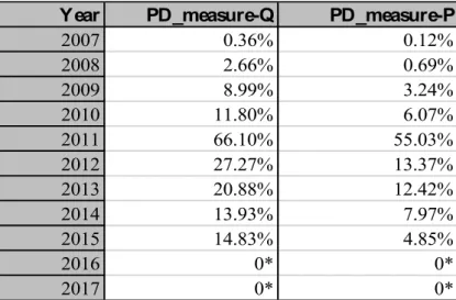
Year PD_measure-Q PD_measure-P
2007 0.36% 0.12% 2008 2.66% 0.69% 2009 8.99% 3.24% 2010 11.80% 6.07% 2011 66.10% 55.03% 2012 27.27% 13.37% 2013 20.88% 12.42% 2014 13.93% 7.97% 2015 14.83% 4.85% 2016 0* 0* 2017 0* 0*
Table 5 - Probabilities of Default of the Portuguese Sovereign.
Analysing the results obtained for the probability of default of the Portuguese sovereign, one is able to see that the values obtained using the probability measure-P are lower than the ones obtained using the probability Q. As previously stated, under the probability measure-Q, the investors are considered risk neutral. Being so, the probability of negative events is higher, as they are not averse to the risk. The probability measure-P, on the contrary, is considered to be the real-world probability. In order to better understand the evolution of these probabilities over time, the results from TABLE 5 were plotted below.
Figure 6 – 5-year Probabilities of Default of the Portuguese Sovereign.
FIGURE 6 presents the evolution of the probabilities of default of the Portuguese Sovereign
over time. As one is able to observe, the values of both probabilities show the same variation – when one of them increased or decreased, the other followed the same pattern. Also, in the time period between 2010 and 2012, the two measures increased severally. This is because of the Portuguese Sovereign debt financial crisis of 2010-2014. In fact, in 2011, as a result of the crisis and the high level of borrowing costs, Portugal was forced to request external financial support. As well as this, Portugal agreed to an economic adjustment program, which required to adopt austerity measures. This was not the only aspect that negatively affected the Portuguese Sovereign. In late March/April of 2011, Fitch lowered Portugal’s rating from A+ to BBB- and Standard and Poor’s from A- to BBB-. With the combination of these two factors, Portugal was forced to request assistance from the international lenders. These are, between others, the main factors that justify why the two probabilities of default rose severally for the time period between 2010-1012.
Finally, for the years 2015-2016, the probabilities of default obtained were extremely close to zero. This is due to the fact that, in 2015, the Portuguese economy started gradually to regain its economic competitiveness.
To further analyse the obtained results, the difference between the two probabilities was calculated and the plot is shown below, in FIGURE 7.
0,00% 20,00% 40,00% 60,00% 80,00% 100,00% 120,00% 140,00% 2007 2008 2009 2010 2011 2012 2013 2014 2015 2016 2017 Pro b ab ili ty o f d ef au lt Year
5-year Probabilities of Default of the Portuguese Sovereign
Figure 7 - Difference between PDs.
The variation of the two PDs over time followed the same pattern as the one from each probability of default individually. This is because the two evolved in the same way. This difference between the two can be interpreted as being the Market Price of Risk. The higher the Market Price of Risk, the Higher should the difference between the two Probabilities of Default be.
Figure 8 - Evolution of the PDs difference for each MPDR.
As one can observe from FIGURE 8, this relationship is not strictly ascending. This happened because there were years for which the firms’ Market Price of Diffusion Risk was high, but the Sovereign’s credit risk was relatively low. The fact that the probability of default is low makes
0,00% 2,00% 4,00% 6,00% 8,00% 10,00% 12,00% 14,00% 16,00% 2007 2008 2009 2010 2011 2012 2013 2014 2015 2016 2017 Pro b ab ili ty o f De fau lt Years
Difference between PDs
0,00% 2,00% 4,00% 6,00% 8,00% 10,00% 12,00% 14,00% 16,00% 15,29% 16,38% 19,40% 21,20% 23,92% 26,77% 27,41% 28,80% 34,59% Pro b ab ili ties o f Def au lt d if fe re n ce MPDRthe difference between the two measures lower. Even though, the important conclusion that can be taken is that the higher the MPDR, the bigger the difference between the two measures of the probability of default.
All the codding used to obtain the results previously analysed is shown in APPENDIX 5.
CHAPTER 7: CONCLUSIONS
This thesis employed a structural credit risk model to study the Portuguese Sovereign’s probability of default. These models can outperform others based on accounting information because they incorporate forward-looking information embedded in asset prices. In addition, by using this type of model, it is possible to link several fundamental characteristics of the sovereign with its probabilities of default.
The results obtained from the sovereign are in line with what was expected beforehand. Using the same model as the one assumed for firms, although for the Sovereigns the state variable was the government revenue, using the MPDR obtained from the firms, and assuming that 𝜇𝛿𝑔𝑜𝑣 = 0, a function to price the Portuguese Credit Default Swaps was computed. This assumption is valid due to the fact that the sovereign’s debt was assumed to be constant. The main idea here is to assume that the expected value of the debt ratio is constant. Assuming a recovery rate of 40% and comparing the CDS of the model with the observed 5-year CDS, the 𝜌 was extracted, which enabled the calculation of the Probabilities of Default of the Portuguese sovereign, in both probability measures P and Q. The results here obtained are also in line with what was expected, as, firstly, the Probabilities of Default obtained under measure-Q are higher than the ones obtained under probability measure-P, due to risk aversion. Furthermore, the evolution of the two variables over time was also what was predicted – its values rose severally between 2010 and 2012, as a result of the sovereign debt crisis that Portugal went through. Also, to
higher values of the PDs’ difference corresponded higher values of the MPDR, which enforces the fact that the difference between the two PDs is the MPDR. Summing up, the model retrieved values that are close to reality, not only in absolute values, but also regarding their evolution over the time considered.
The results obtained for the firms are also the ones expected. Firstly, information regarding quoted firms was used in order to extract the Market Price of Diffusion Risk, and the year average was calculated. To do so, the 𝜇𝛿, representing the growth rate of the state variable (the CFO for the firms’ case), was firstly calculated. The MPDR for the Portuguese firms showed the variation that was expected, by retrieving low values for the period between 2001 and 2007, increasing its value for the period of the economic and financial crisis that Portugal went through, and decreasing afterwards. It was then assumed that the MPDR for the firms was the same as the one for the Sovereigns. This can be justified by the fact that both firms and the government have their returns affected by the economy of the country. So, they are contingent claims on the same factor (Jeanneret, 2012).
Even though, this thesis has some limitations, regarding the model itself and the data used for the estimations. Staring with the model, it was assumed that the Sovereign and the firms followed a Geometric Brownian Motion. So, returns are normally distributed, meaning that there is a low probability of extreme events. This problem could be solved if one had incorporated jumps in the state variable process.
As for the estimation of the model, several assumptions were also made. These can represent limitations for this study. Firstly, in this model, the CDS spread was assumed to be paid continuously over time, though, in reality, these payments are discrete. Furthermore, it was assumed that the 𝜇𝛿 of the government was zero. This can happen since debt was assumed to be constant, although, it is not what is seen in reality. Another important assumption that was made in order to run this study was to assume that the Market Price of Risk applied to the sovereign was the same as the one applied to the quoted firms. This was the assumption that made it possible to disentangle between the risk-neutral probability of default and the true one. On the empirical part of the study, the main limitation of this thesis is the number of firms used to extract the market price of risk and the extent for which the model was applied. Only one
country was used – Portugal – and, from it, only 6 firms were considered. The reason behind it was due to the fact that the model was extremely sensitive to the magnitude of the values, as well as its variation. So, the model was not able to run with some data from certain firms, and that is the reason why, at the end, only 6 firms were considered. This made the final results too much dependent of individual firms. In spite of the small number of firms, the average market price of across the estimation period is in line with what was expected.
In sum, despite having some limitations this thesis has been able to present and implement a structural credit risk model able to provide estimates on, the probability of default of the Portuguese Sovereign. This approach turned out to be a good alternative to more traditional credit risk models based on accounting information, as this model uses information that is forward looking and incorporated the agents’ expectations, being the results obtained more robust. In addition, in contrast to reduced form models, this approach is able to establish a clear link between the sovereign revenues and expenses and its probability of default.
CHAPTER 8: REFERENCES
Altman, E. I. (1968). The Prediction of Corporate Bankruptcy: A Discriminant Analysis. The
Journal of Finance, 23(1), 193–194.
Altman, E. I., Haldeman, R. G., & Narayanan, P. (1977). ZETA analysis A new model to identify bankrupcy risk of corporations. Journal of Banking and Finance, 1(1), 29–54. Beaver, W. H. (1966). Financial Ratios As Predictors of Failure. Journal of Accounting
Research, 4(1966), 71–111.
Black, F., & Cox, J. C. (1976). Valuing Corporate Securities: Some Effects of Bond Indenture Provisions. The Journal of Finance, 31(2).
Black, F., & Scholes, M. (1973). The pricing of options and corporate libilities. The Journal of Political Economy, 81(3), 637–654.
Brigo, D., Dalessandro, A., Neugebauer, M., & Triki, F. (2007). A Stochastic Processes Toolkit for Risk Management. Fitch Solutions: Quantitative Research.
Brockman, P., & Turtle, H. J. (2003). A barrier option framework for corporate security valuation. Journal of Financial Economics, 67(3), 511–529.
Calin, A. C., & Popovici, O. C. (2014). Modeling Credit Risk Through Credit Scoring.
Internal Auditing & Risk Management, 2(34), 99–110.
Chesney, M., & Morisset, J. (1992). Measuring the Risk of Default in Six Highly Indebted
Countries.
Claessens, S., & Pennacchi, G. (1996). Estimating the Likelihood of Mexican Default from the Market Prices of Brady Bonds. Journal of Financial and Quantitative Analysis,
31(1), 109–126.
Coudert, V., & Gex, M. (2010). Credit default swap and bond markets: which leads the
other? Financial Stability Review.
Duan, J. C. (1994). Maximum likelihood estimation using price data of the derivative contract. Mathematical Finance, 4, 155–167.
Duan, J. C. (2000). Correction: Maximum likelihood estimation using price data of the derivative contract. Mathematical Finance, 10, 461–462.
Duan, J. C., Gauthier, G., & Simonato, J. G. (2004). On the equivalence of the KMV and
maximum likelihood methods for structural credit risk models.
Eom, Y. H., Helwege, J., & Huang, J. Z. (2004). Structural models of corporate bond pricing: An empirical analysis. Review of Financial Studies, 17(2), 499–544.
Forte, S. (2011). Calibrating structural models: a new methodology based on stock and credit default swap data. Quantitative Finance, 11(12), 1745–1759.
Forte, S., & Lovreta, L. (2012). Endogenizing exogenous default barrier models: The MM algorithm. Journal of Banking and Finance, 36(6), 1639–1652.
Friedman, T. L. (1995). Foreign Affairs; Don’t Mess With Moody’s. New York Times. Gapen, M., Gray, D., Lim, C. H., & Xiao, Y. (2008). Measuring and Analyzing Sovereign
Risk with Contingent Claims. IMF Staff Papers, 55(1), 109–148.
Goldstein, R. S., Ju, N., & Leland, H. E. (2001). An EBIT-Based Model of Dynamic Capital Structure. Journal of Business.
Gray, D. F., Merton, R. C., & Bodie, Z. (2007). Contingent claims approach to measuring and managing sovereign credit risk. Journal of Investment Management, 5(4), 5.
Jarrow, R., & Turnbull, S. (1995). Pricing Derivatives on Financial Securities Subject to Credit Risk. Journal of Finance, 50(1), 53–85.
Jeanneret, A. (2012). The dynamics of sovereign credit risk. Journal of Financial and
Quantitative Analysis (JFQA)
Jones, P., Mason, S., & Rosenfeld, E. (1984). Contingent Claim Analysis of Corporate Capital Structures: An Empirical Investigation. Journal of Finance, 39, 611–625.
Lee, H.-H., Shih, K., & Wang, K. (2016). Measuring sovereign credit risk using a structural model approach. Review of Quantitative Finance and Accounting, 47(4), 1097–1128. Leland, H. E. (1994). Corporate Debt Value, Bond Covenants, and Optimal Capital Structure.
Journal of Finance.
Leland, H. E., & Toft, K. B. (1996). Optimal Capital Structure, Endogenous Bankruptcy, and the Term Structure of Credit Spreads. The Journal of Finance, 51(3).
Longstaff, F. A., & Schwartz, E. S. (1995). A Simple Approach to Valuing Risky Fixed and Floating Rate Debt. The Journal of Finance, 50(3).
Martin, R., Xu, H., Koch, F. J., & Guo, S. (2007). Cusp 2007. Credit Suiss Research and
Analytics.
Merton, R. C. (1974). On the Pricing of Corporate Debt: The Risk Structure of Interest Rates.
The Journal of Finance.
Ronn, E. I., & Verma, A. K. (1986). Pricing Risk-Adjusted Deposit Insurance: An Option-Based Model, 48(4), 1231–1262.
Sundaresan, S. (2013). A Review of Merton’s Model of the Firm’s Capital Structure with Its Wide Applications. Annual Review of Financial Economics, 5(1), 21–41.
Vasicek, O. (1977). An Equilibrium Characterization of the Term Structure. Journal of
Financial Economics, 5, 177–188.
Vassalou, M., & Xing, Y. (2004). Default Risk in Equity Returns. The Journal of Finance,
Wang, H. Y., & Li, K. L. (2004). On Bias of Testing Merton’s Model. The Chinese University
of Hong Kong Working Paper, 82–90.
Zhou, C. (2001). An Analysis of Default Correlation and Multiple Default. The Review of
CHAPTER 9: APPENDIX
Appendix 1
The value of the coupon leg in Equation (3.5) can be computed as follows:
𝐶𝑜𝑢𝑝𝑜𝑛𝐿𝑒𝑔(𝑡𝑐𝑑𝑠, 𝐿𝑐𝑑𝑠) = 𝐿 ∗ 𝜛{𝑒 𝜛𝑡𝑐𝑑𝑠(1 − 𝑁(ℎ 1(𝑣,̅ 𝑡𝑐𝑑𝑠)) − 𝑅2𝑎𝑁(ℎ2(𝑣,̅ 𝑡𝑐𝑑𝑠)) − 1 + 𝐹 (𝜛,ln(𝑅) 𝜎 , 𝑣 𝜎, 𝑡 𝑐𝑑𝑠) + 𝑅2𝑎𝐹 (𝜛,ln(𝑅) 𝜎 , − 𝑣 𝜎, 𝑡 𝑐𝑑𝑠)} Where 𝑅 =𝑣̅ 𝐴 ℎ1(𝑧, 𝑠) =ln ( 𝑧 𝐴) − 𝑣𝑠 𝜎√𝑠 ℎ2(𝑧, 𝑠) = ln (𝑅𝑧 𝑣̅) + 𝑣𝑠 𝜎√𝑠 𝑎 = 𝑣 𝜎2 𝜛 = −𝑟 𝑣 = 𝜇𝛿− 𝑀𝑃𝐷𝑅 ∗ 𝜎 − 0.5𝜎2 𝐹(𝑎, 𝑏, 𝑐, 𝑦) = {Ω𝑔 +(𝑎, 𝑐)𝑔+(𝑦)+ Ω ℎ +(𝑎, 𝑐)ℎ+(𝑦), 𝑏 > 0 Ω𝑔−(𝑎, 𝑐)𝑔−(𝑦)+ Ωℎ−(𝑎, 𝑐)ℎ−(𝑦), 𝑏 < 0 Ω𝑔±(𝑎, 𝑐) = ∓ √𝑐2− 2𝑎 ∓ 𝑐 2√𝑐2− 2𝑎 Ωℎ±(𝑎, 𝑐) == ∓√𝑐 2− 2𝑎 ∓ 𝑐 2√𝑐2− 2𝑎
𝑔±(𝑦) = 𝑒∓𝑏Ψ𝑔±(𝑎,𝑐)𝑁 (∓𝑏 − √𝑐 2− 2𝑎𝑦 √𝑦 ) ℎ±(𝑦) = 𝑒∓𝑏Ψℎ±(𝑎,𝑐)𝑁 (∓𝑏 − √𝑐2− 2𝑎𝑦 √𝑦 ) Ψ𝑔±(𝑎, 𝑐) = ∓𝑐 − √𝑐2− 2𝑎 Ψℎ±(𝑎, 𝑐) = ∓𝑐 − √𝑐2− 2𝑎
Regarding Equation (3.6), we have that
𝐸𝐿𝑡𝑜 𝑐𝑑𝑠 = 𝐿𝑐𝑑𝑠𝐹 (𝜛,𝑙𝑛(𝑅) 𝜎 , 𝑣 𝜎, 𝑡 𝑐𝑑𝑠) + 𝑅2𝑎𝐹 (𝜛,𝑙𝑛(𝑅) 𝜎 , − 𝑣 𝜎, 𝑡 𝑐𝑑𝑠) −𝐿𝑐𝑑𝑠 𝐿∗ 𝛽𝑉𝐵𝐹 (𝜛, 𝑙𝑛 (𝑅) 𝜎 , 𝑣 𝜎, 𝑡 𝑐𝑑𝑠) + 𝑅2𝑎𝐹 (𝜛,𝑙𝑛 (𝑅) 𝜎 , − 𝑣 𝜎, 𝑡 𝑐𝑑𝑠).
he probability of default in measures Q and P is given by:
𝑃𝐷(𝑇) = 𝐸ℚ[1𝑠<𝑇] = 𝐹 (0,ln (𝑅) 𝜎 , 𝑣 𝜎, 𝑠) + 𝑅 2𝑎𝐹 (0,ln (𝑅) 𝜎 , − 𝑣 𝜎, 𝑠) 𝑃𝐷(𝑇) = 𝐸ℙ[1 𝑠<𝑇] = (0, ln (𝑅) 𝜎 , 𝑣𝑃 𝜎 , 𝑠) + 𝑅 2𝑎𝐹 (0,ln (𝑅) 𝜎 , − 𝑣𝑃 𝜎 , 𝑠) where 𝑣𝑃 = 𝑣 + 𝑀𝑃𝐷𝑅 ∗ 𝜎