Finite Elements in Analysis and Design 165 (2019) 52–64
Contents lists available atScienceDirect
Finite Elements in Analysis and Design
journal homepage:www.elsevier.com/locate/finelA continuous-stress tetrahedron for finite strain problems
P. Areias
a,b,e, T. Rabczuk
f,∗, F. Carapau
c,e, J. Carrilho Lopes
d,eaCERIS/Instituto Superior Técnico, University of Lisbon, Portugal bDepartment of Physics, Portugal
cDepartment of Mathematics and CIMA, Portugal dDepartment of Geosciences, Portugal
eUniversity of Évora Colégio Luís António Verney Rua Romão Ramalho, 59 7002-554, Évora, Portugal fInstitute of Structural Mechanics Bauhaus-University, Weimar Marienstraße, 15 99423, Weimar, Germany
A R T I C L E I N F O
Keywords:
Hellinger-reissner variational principle Tetrahedron
Continuous stress Finite strains Inf-sup
A B S T R A C T
A finite-strain tetrahedron with continuous stresses is proposed and analyzed. The complete stress tensor is now a nodal tensor degree-of-freedom, in addition to displacement. Specifically, stress conjugate to the relative Green-Lagrange strain is used within the framework of the Hellinger-Reissner variational principle. This is an extension of the Dunham and Pister element to arbitrary constitutive laws and finite strain. To avoid the excessive conti-nuity shortcoming, outer faces can have null stress vectors. The resulting formulation is related to the nonlocal approaches popularized as smoothed finite element formulations. In contrast with smoothed formulations, the interpolation and integration domain is retained. Sparsity is also identical to the classical mixed formulations. When compared with variational multiscale methods, there are no parameters. Very high accuracy is obtained for four-node tetrahedra with incompressibility and bending benchmarks being successfully solved. Although the ad-hoc factor is removed and performance is highly competitive, computational cost is high, as each tetrahedron has 36 degrees-of-freedom. Besides the inf-sup test, four benchmark examples are adopted, with exceptional results in bending and compression with finite strains.
1. Introduction
Numerical analysis [8] and applied mathematics analysis [12] have long agreed on the solutions for locking of low-order elements under quasi-incompressible (and incompressible) conditions. Mixed displacement-pressure formulations passing the inf-sup stability condi-tion are currently well established, as are solucondi-tions for circumventing this condition, cf. [26], which developed into the variational multiscale techniques [1,32,50] now in widespread use with virtually all consti-tutive laws. More traditional formulations, such as the MINI formula-tion (continuous pressure+bubble-enriched displacement) [6] and its variants [46] are now still adopted [4] in combination with other tech-niques, see also [31,41].
Accuracy and stability in the quasi-incompressible case are now well understood (see, e.g. Ref. [7]). Another related goal is the high coarse-mesh accuracy in the sense of Belytschko and Bachrach [10] in partic-ular when bending is involved. For hexahedra, high coarse-mesh
accu-∗Corresponding author.
E-mail address:[email protected](T. Rabczuk).
rate elements for finite strains are available [5,43,49] and only incre-mental developments are being performed to improve specific aspects, for example stability under compression.
High coarse-mesh accurate tetrahedra are difficult to produce as bending modes cannot be directly added with the incompatible mode method. The closest to a bending-enhanced tetrahedron is the rotation-based tetrahedron by Nodargi et al. [35].
An alternative to enrichment consists in increasing the integra-tion domain by creating pseudo-elements based on tetrahedra shar-ing a node, an edge or a face. This smoothed finite element tech-nology has been extensively explored recently. For node smoothing, stabilization is required [14,19,21,29,38], for edge smoothing [23,37] and face smoothing [33] stabilization is not required. However, in all three smoothing options, Jacobian densification occurs (cf.Fig. 8of [21]) and the conventional finite element implementation is disrupted. Although intricate to implement, smoothing strategies result in greatly improved bending performance. Incompressibility is however a
differ-https://doi.org/10.1016/j.finel.2019.07.003
Received 25 February 2019; Received in revised form 18 June 2019; Accepted 17 July 2019 Available online 20 August 2019
Algorithm 1 Relative Lagrangian formulation (Voigt notation adopted) for elasto(visco) plastic materials. Frame b, reference configurationΩband equilibrium configurationΩa.
Input data Giveneb
ab(Voigt form) R00′and R0b
Recover from storageS0
b0ande
0
b0
Frame change from 0 to b and stress/strain updating
Accumulated Green-Lagrange strain in frame b ebb0=e
( RT0b)e0b0
Right stretch tensor for configurationΩb Ubb0=
√ 2eb
b0+I Jb0=det U b b0
Deformation gradient in frames b − b Fbbb0=RT00′R0bUbb0
Deformation gradient in frames b − 0 Fb0b0=Fbbb0RT0b
Update total strain in frame b eb
a0=e b b0+e [( Fbb b0 )T] eb ab Stress in frame b Sbbb=J1 b0s ( Fb0b0)S0b0 Determine stress Sb ab=S b bb+ ΔŠa ( eb ab ) and sensitivity ab=𝜕Δ𝜕eŠba ab
Determine the total strain in frame 0 e0
a0=e(R0b)eba0
Determine the second Piola-Kirchhoff stress in frame 0 S0
a0=Jb0s [( Fb0 b0 )−1] Sb ab StoreS0a0ande0 a0
Return to the elementSb ab,ab
ent matter and some of the recent smoothed finite elements include internal bubbles to avoid locking in the incompressible limit, see Refs. [34,36].
We here take a different approach. By using the Hellinger-Reissner variational principle (cf [8,24]), we proposed a stress and displacement-based element for finite strains which can be viewed as an exten-sion of the linear formulation by Dunham and Pister [20] to deal with any constitutive law in finite strains. With that goal, a spe-cific constitutive updating algorithm is used, filling the technical aspects required to extend the small strain formulation to finite strains. Although computational cost is significant, and the stiffness matrix is unsymmetrical, at the node level, system sparsity is the same as with a displacement-based element and implementation is straightfor-ward.
The manuscript is organized as follows: Section2presents the con-stitutive updating algorithm, which is adopted by our tetrahedron for-mulation, described in Section3. Section3also shows the convergence of the inf-sup parameter for a block mesh. Section4presents 4 bench-marks to assess the performance of the new element and finally, in Section5draws the conclusions, with a discussion on the advantages and shortcomings of the present element.
2. Constitutive updating
To use a common equilibrium formulation for hyperelasticity and rate-based finite-strain elasto-plasticity is a difficult task, especially when using mixed formulations. For specific pressure/displacement [45] or enhanced strain formulations [5,42,43], this can be performed with multiplicative decomposition of the deformation gradient, FeFp
[44]. It is intricate to ensure frame-invariance as sharply noted by Glaser and Armero [22]. However, when stress nodal
degrees-of-freedom are present, ambiguities would occur due to the required trans-formations performed at the element level.
Relative strain measures are therefore convenient for the assumed stress formulation employed in this work. ConfigurationΩ0is the
ini-tial configuration,Ωbas the reference configuration andΩaas the
equi-librium configuration. To these three configurations we associate three frames 0,b and a, respectively. We introduce local frame 0′ correspond-ing to the local undeformed configurationΩ0. Therefore, for
configura-tionΩ00 is the global frame and 0′is the local frame. A given tensor T is
written, in frame c for reference configurationΩband equilibrium
con-figurationΩaas Tcab. When the frame is obvious or of no consequence,
we omit the superscript c.
After introducing the relative deformation gradient between config-urationsΩbandΩaas Fabwe have:
Fab=Fa0F−b01 (1)
The Green-Lagrange strain between configurations is obviously eab=
1 2
(
FTabFab−I
)
and therefore we can write:
ea0=eb0+FTb0eabFb0 (2)
If a frame b is identified by the basis vectors g1b,g2b and g3b written in frame 0 by column, we can write the frame matrix for b as R0b=
[
g1b∣g2b∣g3b
]
. This frame matrix for the reference configuration is of course relevant for structural elements, but also anisotropic continuum elements where a frame-of-reference is required. An initial frame (0′) is used for structural elements so that in general R00′≠ I. Of course,
although frames are distinct, configurations coincideΩ0≡Ω0′.Change
of frame of a given second-order tensor T is obtained in general as: Ta=RabTbRTab. Polar decomposition of the deformation gradient Fa0is
obtained from the rotation and stretch Ua0:
Fa0=R0′aUa0 (3)
In the particular case of the deformation gradient, which is a two-point tensor, we have the following change of frames transformation, see also [30]:
Fcdab=RceFefabRfd (4)
Which allows the writing of Fa0in frames b − 0 as Fb0
a0=Rb0F00a0 (5)
This formula is relatively standard [47] and supports the classical coro-tational method, which here is identified as: Fb0b0=U0b0. Having defined the relative Green-Lagrange strain eab, which is the traditional
Green-Lagrange strain assuming that the initial configuration isΩb, we now
use the power conjugacy between the Green-Lagrange strain rate (e)̇ and the second Piola-Kirchhoff stress (S) to obtain:
∫Ωa S∶eḋ Ωa= ∫Ω0 Sa0∶ėa0dΩ0= ∫Ωb Sab∶ėabdΩb (6) from which we obtain the following relation:
Sab=J1 b0
Fb0Sa0FTb0 (7)
where Jb0 = detFb0. Generalizing, we have:
Sac= 1 Jcb
FcbSabFT
cb (8)
The Cauchy stress, for example, is identified as Saa and follows the
traditional formula: Saa=J1
ab
FabSabFTab (9)
We therefore have two choices concerning the constitutive updating at finite strains within this framework:
•Hyperelasticity with frame b: Sb a0
( eb
a0
)
•Hypoelasticity/inelastic materials with frame b: Sb ab=S b bb+ Δ̌Sa ( eb ab )
whereΔ̌Sais the incremental stress.
Algorithm 1 summarizes the steps (here only for hypoelasticity), where use is made of Voigt form for symmetric tensors:
Voigt ⎡ ⎢ ⎢ ⎢ ⎣ S11 S12 S13 S12 S22 S23 S13 S23 S33 ⎤ ⎥ ⎥ ⎥ ⎦ = ⎧ ⎪ ⎪ ⎪ ⎪ ⎨ ⎪ ⎪ ⎪ ⎪ ⎩ S11 S22 S33 S12 S13 S23 ⎫ ⎪ ⎪ ⎪ ⎪ ⎬ ⎪ ⎪ ⎪ ⎪ ⎭ ⇔ (10) Voigt[S] =S (11)
We use upright bold format for symmetric tensors represented in Voigt format and the usual slanted bold format for tensors in conventional format.
Omitting the configuration and frame indices, the terms(F)is
cal-culated as: s(F) = ⎡ ⎢ ⎢ ⎢ ⎢ ⎢ ⎢ ⎢ ⎢ ⎢ ⎣ F112 F212 F312 2F21F11 2F31F11 2F31F21 F2 12 F222 F322 2F22F12 2F32F12 2F32F22 F132 F232 F332 2F23F13 2F33F13 2F33F23 F11F12 F21F22 F31F32 F21F12+F11F22 F31F12+F11F32 F31F22+F21F32 F11F13 F21F23 F31F33 F21F13+F11F23 F31F13+F11F33 F31F23+F21F33 F12F13 F22F23 F32F33 F22F13+F12F23 F32F13+F12F33 F32F23+F22F33 ⎤ ⎥ ⎥ ⎥ ⎥ ⎥ ⎥ ⎥ ⎥ ⎥ ⎦ ande(F) =Ts(F T).
3. Stress-displacement formulation for the tetrahedron
Specific applications, as well as quasi-incompressible constitutive laws, expose the limitations of low-order displacement-based tetrahe-dra. For an extensive period of time, traditional low-order mixed ele-ments were a solution for avoiding locking in quasi-incompressible problems. Although quasi-incompressible and incompressible materials are well served by mixed u − p elements satisfying the inf-sup condi-tion (see, the descripcondi-tion by Bathe [8]), bending and torsion are not. If only quasi-incompressible materials are of interest, the MINI formu-lation by Douglas Arnold ([6]), see also Bathe [8] and Cao [15] is a reliable solution with low-order interpolation.
However, to improve on results in bending, we use stress tensor interpolation in a form not distinct from the work of Dunham and Pis-ter [20] in finite strains. Here the two-field Hellinger-Reissner varia-tional principle [24] is adopted. Stress and displacement, as in the orig-inal Hellinger-Reissner principle, are the independent fields, with stress being the primary. We therefore introduce the independent stress̃Sabas
a nodal degree-of-freedom.
• Stresses are linearly interpolated using the corner nodes.
• Relative strain rates and conjugate stresses are employed.
We start with the complementarity strain energy density Uc(̃S ab
) which is used in the Hellinger-Reissner functional (in Voigt form [48]):
ΠHR ( ̃ Sab,u ) = − ∫Ωb Uc(̃S ab ) dΩb+∫ Ωb ̃Sab·eab(u)dΩb−Wext(u) (12) where dependence on the stress̃Sab and the displacement u is made explicit. In (12), Wext(u)is the work of conservative external forces.
Stationarity of (12) with respect tõSaband u is made here by using a
time-derivative. Hence, ̇ΠHR(̃Sab,u ) =∫ Ωb [ eab(u) −̃eab ] · ̇̃SabdΩb + ∫Ωb ̃ Sab·˙eab(u)dΩb− ̇Wext(u) =0 (13) with̃eab=dU c(̃S ab ) d̃Sab
. Partitioning the terms dependent onu and thė terms dependent onṠ̃ab, we obtain (omitting the argument u):
∫Ωb ̃ Sab·˙eabdΩb= ̇Wext (14) ∫Ωb [ eab(u) −̃eab ] · ̇̃SabdΩb=0 (15)
We now make use of a tangent relationṠ̃ab=· ̇̃eab where the
tan-gent modulus is obtained from Uc as=
[ d2Uc(̃S ab ) d̃S2ab ]−1 . By using
Fig. 1. Inf-sup test (𝛾h), free boundary conditions. Convergence curve for𝛾h. ̇𝝀 = −ẽ̇abwe obtain, by usingeab(u) −ẽab=0⇒ Sbab− ̃Sab=0, ∫Ωb [( ̃ Sab−Sbab ) · ̇𝛌]dΩb=0 (16)
In terms of power balance, we use the following relation, wherẽSabis
independent of the displacement field. Weak form corresponds to the following stationarity condition:
∫Ωb ̃Sab·ėabdΩb+∫ Ωb [( ̃ Sab−Sbab ) · ̇𝛌]dΩb ⏟⏞⏞⏞⏞⏞⏞⏞⏞⏞⏞⏞⏞⏞⏞⏞⏞⏞⏞⏞⏞⏞⏞⏞⏞⏞⏞⏞⏞⏞⏞⏞⏞⏟⏞⏞⏞⏞⏞⏞⏞⏞⏞⏞⏞⏞⏞⏞⏞⏞⏞⏞⏞⏞⏞⏞⏞⏞⏞⏞⏞⏞⏞⏞⏞⏞⏟ ̇ Wint = ̇Wext (17) whereSb
ab is the constitutive-based stress and𝝀 is now identified as
the Lagrange multiplier required to impose, in the weak form, the con-straint
̃Sabweak̃=Sbab (18)
In (17),Ẇextis the external work power, obtained by the internal
prod-uct of external forces with the corresponding velocities: ̇ Wext=∫ Ωb ̇ u·bdΩb+∫ Γt ̇ u·tdΓt (19)
whereu is the velocity vector, b is the external body force and t is thė stress vector at boundaryΓt. Using time-derivatives, in (17), we have ̇𝛌
as the Lagrange multiplier “velocity” conjugate to the stress.
Table 1
Values of𝛾hfor𝜈 = 0.3,𝜈 = 0.499 and
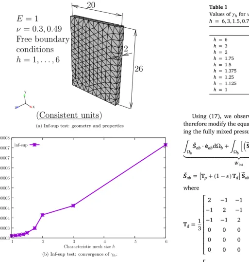
h= 6,3,1.5,0.75 𝜈 =0.3 𝜈 =0.499 h= 6 7.1478×10⁻⁵ 7.1478×10⁻⁵ h= 3 4.1122×10⁻⁵ 4.1122×10⁻⁵ h= 2 3.6516×10⁻⁵ 3.6516×10⁻⁵ h= 1.75 2.9895×10⁻⁵ 2.9895×10⁻⁵ h= 1.5 2.7571×10⁻⁵ 2.7571×10⁻⁵ h= 1.375 2.6827×10⁻⁵ 2.6827×10⁻⁵ h= 1.25 2.6521×10⁻⁵ 2.6521×10⁻⁵ h= 1.125 2.6267×10⁻⁵ 2.6267×10⁻⁵ h= 1 2.6104×10⁻⁵ 2.6104×10⁻⁵
Using (17), we observed near-singularity in certain problems and therefore modify the equations in weak form to stabilize it while retain-ing the fully mixed pressure part of the stress:
∫Ωb Šab·ėabdΩb+∫ Ωb [( ̃ Sab−Sbab ) · ̇𝛌]dΩb ⏟⏞⏞⏞⏞⏞⏞⏞⏞⏞⏞⏞⏞⏞⏞⏞⏞⏞⏞⏞⏞⏞⏞⏞⏞⏞⏞⏞⏞⏞⏞⏞⏞⏟⏞⏞⏞⏞⏞⏞⏞⏞⏞⏞⏞⏞⏞⏞⏞⏞⏞⏞⏞⏞⏞⏞⏞⏞⏞⏞⏞⏞⏞⏞⏞⏞⏟ ̇ Wint = ̇Wext (20) Šab= [ Tp+ (1−𝜀)Td ]̃ Sab+𝜀TdSbab (21) where Td=1 3 ⎡ ⎢ ⎢ ⎢ ⎢ ⎢ ⎢ ⎢ ⎢ ⎢ ⎣ 2 −1 −1 0 0 0 −1 2 −1 0 0 0 −1 −1 2 0 0 0 0 0 0 3 0 0 0 0 0 0 3 0 0 0 0 0 0 3 ⎤ ⎥ ⎥ ⎥ ⎥ ⎥ ⎥ ⎥ ⎥ ⎥ ⎦ Tp=13 ⎡ ⎢ ⎢ ⎢ ⎢ ⎢ ⎢ ⎢ ⎢ ⎢ ⎣ 1 1 1 0 0 0 1 1 1 0 0 0 1 1 1 0 0 0 0 0 0 0 0 0 0 0 0 0 0 0 0 0 0 0 0 0 ⎤ ⎥ ⎥ ⎥ ⎥ ⎥ ⎥ ⎥ ⎥ ⎥ ⎦ (22)
In all examples, we use𝜀 = 5%. The purpose of this modification is to allow a solution during the Newton iteration, and no effort was made in tuning this parameter. Since the pressure termTp̃Sabis independent
of the interpolated displacement, no locking occurs for any value of𝜀. The variation of (20) is required in the application of Newton-Raphson process: dẆ int= ∫Ωb [ Tp+ (1−𝜀)Td]ds̃Sab·ėabdΩb (23) + ∫Ωb 𝜀TdduSb ab·ėabdΩb+∫ Ωb Šab·duėabdΩb (24) + ∫Ωb [( ds̃Sab−duSbab ) · ̇𝛌]dΩb (25)
where dSindicates the variation with respect to the stress
degrees-of-freedom and duindicates the variation with respect to the displacement degrees-of-freedom. For a close inspection of the quantities involved in (17) and (23), we have the relative deformation gradient as a product
Fig. 2. Cube test to assess the computing time.
of the Jacobian for configurationΩawith the inverse of the Jacobian
for configurationΩb:
Fab=JaJ−b1 (26)
Which, introducing the positions at configurationΩaand configuration Ωbas xaand xb, along with a set of curvilinear coordinates𝝃,we obtain: Ja=𝜕xa
𝜕𝝃 (27)
Jb=𝜕 xb
𝜕𝝃 (28)
with the relative displacement being uab = xa−xb. Of course, from
(26), we obtain: eab=12 ( FTabFab−I ) (29) The variation of (29) is given by
dueab=12 [ J−bT(duJTaJa+JTaduJa ) J−b1] (30) where duJa= 𝜕 duxa 𝜕𝝃 (31)
In terms of constitutive stress variation, we have:
duSbab=abdueab (32)
whereab is the constitutive tangent modulus. We now introduce the
interpolations for u,̃Saband𝝀as: u(𝝃) = 4 ∑ K=1 NK(𝝃)uK (33) ̃ Sab(𝝃) = 4 ∑ K=1 NK(𝝃)̃SabK (34) 𝝀(𝝃) =∑4 K=1 NK(𝝃) 𝝀K (35)
We remark that, according to Zienkiewicz, Taylor and Zhu [51], page 296, “…identical interpolation of N𝜎and Nuis acceptable from the point of view of stability.” Shape functions NK(𝝃)for each tetrahedron node K
are written according to their definition (cf [25]):
N1(𝝃) =1−𝜉1−𝜉2−𝜉3 (36a)
N2(𝝃) = 𝜉2 (36b)
N3(𝝃) = 𝜉3 (36c)
N4(𝝃) = 𝜉1 (36d)
Not all quantities are determined by hand-derivation, and we use Mathematica [40] with the AceGen (cf [28]) add-on to calculate some derivatives. Making use of the concepts of Sobolev spaces and norms [13], along with the inf-sup results, we assess the convergence of this element for a simple verification test. We require the L2norm of̃S
ab
and the Sobolev norm‖•‖W1,2(Ω b)of u: ‖‖ ‖̃Sab‖‖‖L2(Ω b) = √ 𝔸e ( ‖̃Sab‖2L2(Ωe b) ) e (37) ‖u‖W1,2(Ω b)= √ √ √ √ √𝔸e ( 1 ∑ |𝜶|=0 ‖𝜕𝜶u‖2 L2(Ωe b) ) e (38) where𝜕𝜶u=𝜕 𝜕|𝜶|u x𝛼1 1 𝜕x 𝛼2 2 𝜕x 𝛼3 3 with|𝜶| = 𝛼1 + 𝛼2 + 𝛼3. In (37),𝔸e is
the assembling operation, described by Hughes [25] withΩebbeing the reference configuration for element e. In terms of components, we have ‖̃Sab‖2L2(Ωe b) =∫ Ωeb 3 ∑ i,j=1 ( ̃Sab )2 ijdΩb (39) 1 ∑ |𝜶|=0 ‖𝜕𝜶u‖2 L2(Ωe b) = ∫Ωe b {3 ∑ i=1 [ [u]2i + 3 ∑ k=1 (𝜕[ u]i 𝜕Xk )2]} dΩb (40)
With (37–38) along with (39–40), we have two discrete quadratic forms for the norms:
Fig. 3. Cantilever beam: relevant data (geometry, boundary conditions and material properties). Contour plot of S0
11stress is also shown for formulations.
‖‖ ‖̃Sab‖‖‖ 2 L2(Ω b) = ̃ST hG̃Sh (41) ‖u‖2 W1,2(Ω b) =u T hTuh (42)
where uh and̃Sh are the displacement and stress global
degrees-of-freedom. We note that G and T are global matrices, similar in terms of assembling to the stiffness matrix. We use the assembling operation to perform this task, as well as AceGen [28] to determine the cliques. To that goal, we use the Hessians of ‖‖‖̃Sab‖‖‖
2 L2(Ω b) and‖u‖2 W1,2(Ω b) to obtain
G and T, respectively. Since stress is the primary field, we assess the stability of this formulation in detail, using the inf-sup parameter fol-lowing Brezzi and Fortin [13] (see Y. Ko and K.-J. Bathe [9,18,27]): 𝛾h=infu h sup ̃Sh uT hKuS̃Sh √ ̃ ST hG̃Sh· √ uT hTuh (43) This definition provides a number𝛾hthat measures the crossed-term in
the stiffness matrix and therefore the strength with which the constraint is imposed. We intentionally omit the spaces in (43) to avoid overload-ing the notation. We now make use of the proof provided by Brezzi and Fortin [11,13] that equates𝛾hto the square-root of the smallest
nonzero eigenvalue𝜆kof the following generalized problem, where𝝓k
are the corresponding eigenvectors: ( KTuST−1KuS ) 𝝓k=𝜆2kG𝝓k (44) We equate𝛾hto min𝜆 k>0
𝜆k, see Brezzi and Fortin [13], proposition 3.1. The
inf-sup condition is now verified for the geometry shown inFig. 1. We
use a characteristic mesh parameter h with values from 1 to 6.Table 1 andFig. 1b show the results. Two conclusions are drawn:
• An horizontal asymptote in𝛾his detected showing the convergence
of this formulation.
• The Poisson coefficient does not affect the value of𝛾h, a fact that is confirmed in the numerical examples.
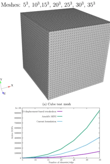
In terms of computational cost, we select the most demanding case for sparsity, a cube represented in Fig. 2. A single linear analysis is performed, with upper and bottom faces of the cube being clamped. Meshes with up to 35 elements per edge are adopted. A Clevo Laptop is used, with a 6-core Intel i7-8700 K processor and 32 GB of 2400 MT/s RAM. Our linear frontal solver is used, cf [3].Fig. 2b shows the relation between the number of degrees-of-freedom and the number of elements per edge with elements T4, MINI, and our formulation. We note that in the MINI element, internal degrees-of-freedom are accounted. Clock time vs the number of elements per edge is shown inFig. 2c. We note that computational cost is significant, which is consequence of using 9 degrees-of-freedom for each node and the stiffness matrix is unsymmet-rical.
4. Numerical tests
Four numerical experiments are now performed, with a cantilever beam, Cook’s membrane, asymmetric compression and the classical drilled plate under tension. The objective is two-fold: verification of the implementation and benchmarking. For comparison, results from the
Fig. 5. Cook’s membrane: geometry, boundary conditions and constitutive properties.
literature are shown, and critically compared with the ones produced by our formulation. Our SimPlas software (cf [2]) is employed for all examples.
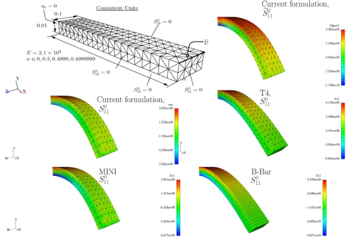
4.1. Cantilever beam, Kirchhoff/Saint-Venant constitutive law
Bending tests are especially demanding for tetrahedra element tech-nology when coarse meshes and incompressibility are present. With the goal of assessing the improvements resulting from the current
formula-tion, we present a cantilever beam, seeFig. 3with prescribed vertical displacement at the top edge of the beam extremity. Also shown in Fig. 3are contour plots of the stress component̃S0
11.
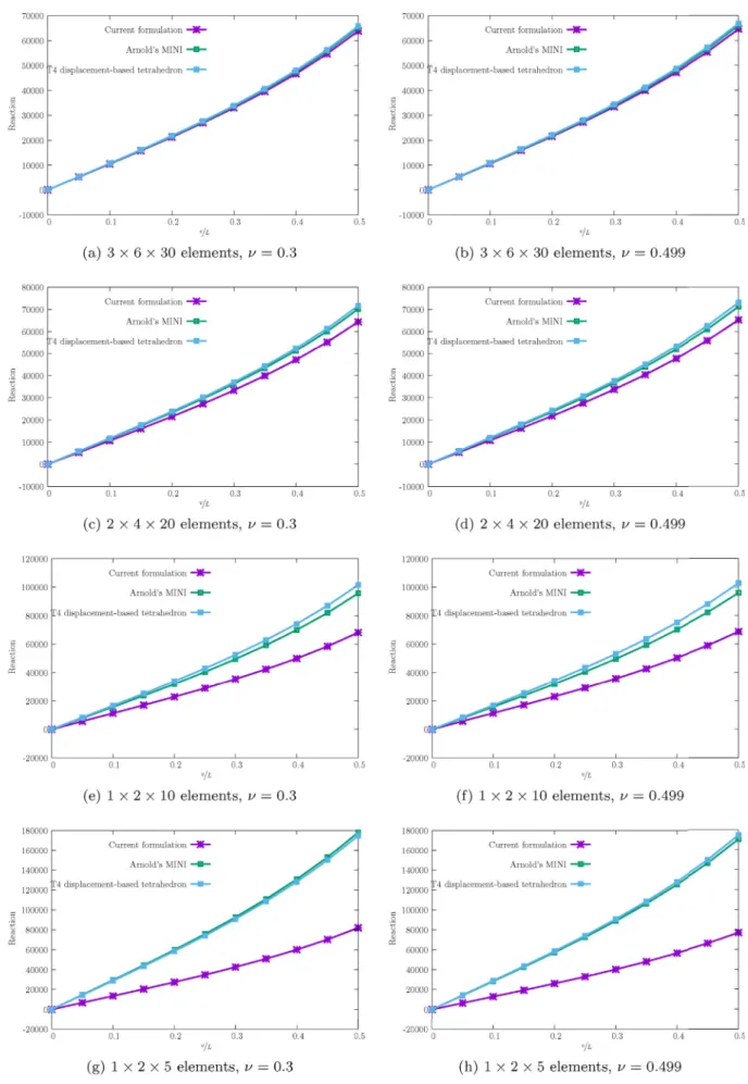
Results for increasingly coarse meshes are shown inFig. 4. Meshes with 3 × 6 × 30, 2 × 4× 20, 1 × 2 × 10 and 1 × 2× 5 ele-ments are employed, with two Poisson coefficients: 𝜈 = 0.3 and 𝜈 = 0.499. We observe that, for coarse meshes, the present formu-lation clearly outperforms the T4 (textbook implementation of the displacement-based tetrahedron element) and Arnold’s MINI element.
Fig. 6. Cook’s membrane results.
Coarser meshes greatly benefit the present formulation, especially for 𝜈 = 0.499.
4.2. Cook’s membrane
We now apply the formulation to the Cook’s membrane problem (the 2D version is common, cf [32,42]). A 3D linear version was adopted by Mahnken, Caylak, and Laschet [31]. This problem combines incom-pressibility and bending, which are both especially demanding for low-order tetrahedra. We use two constitutive laws: Neo-Hookean elasticity and J2elasto-plasticity, as described by Simo and Armero [42] to
inves-tigate the relative merits when compared with classical formulations. Fig. 5shows the relevant data and contour plots for the stress degrees-of-freedom̃S in the elastic and also𝜀p in the elasto-plastic case. Very
smooth stress contour plots are obtained (obviously continuous) which
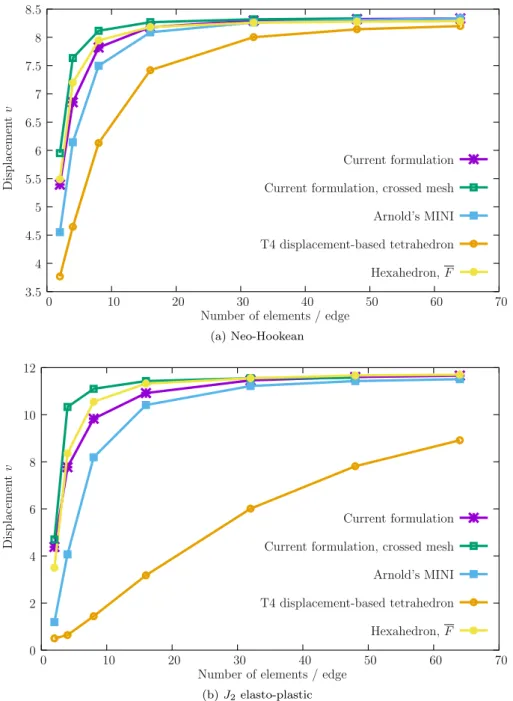
benefits the elasto-plastic analysis. A comparison with the nodally inte-grated tetrahedra, see Ref. [38], for the same example shows an advan-tage in terms of stress smoothness. In Fig. 6, we present the results for Neo-Hookean elasticity (sub-Fig. 6a) and J2elasto-plasticity
(sub-Fig. 6b). For the new formulation, a standard discretization is used and we also test a crossed-mesh (hexahedra divided into 24 tetrahe-dra) with the same density.Fig. 6a shows the tip displacement con-vergence results for the Neo-Hookean case, where a comparison with Arnold’s MINI element [6] and the hexahedron version of Simo, Tay-lor and Pister element [45], here denoted F, is performed. The new formulation produces high quality results, with the crossed-mesh ver-sion outperforming the F hexahedron. As expected by the continuity of stresses, the elasto-plastic benchmark produces excellent results, as Fig. 6b shows. With the crossed-mesh version, our formulation clearly outperforms the F hexahedron in the elasto-plastic test.
Fig. 7. Quasi-incompressible Neo-Hookean compression test.
Fig. 8. Quasi-incompressible Neo-Hookean compression test.
4.3. Quasi-incompressible block under compression
Using a quasi-incompressible hyperelastic law, we test the new for-mulation with a well-known benchmark where an asymmetric compres-sion of a block is performed. The large strain comprescompres-sion test by Reese, Wriggers and Reddy [39] and hyper-elastic a quasi-incompressible Neo-Hookean material law was selected, with the following strain energy density function: Ψ =1 2𝜇 ( tr[Ĉ]−3)+1 2𝜅(log[J]) 2 (45)
In (45), ̂C=J−23C and C=FTF with 𝜅 = 400889.806 and
𝜇 = 80.194 (consistent units). In this example, compressive strains and high strain gradients are combined and this poses severe constraints on the element formulation to use. Geometry, constitutive properties and boundary conditions for this example are shown inFig. 7. One quar-ter of the system is discretized due to the presence of two symmetry planes. In addition, the upper surface is prescribed in the x and z direc-tions. Relevant properties and dimensions for this problem are shown in Fig. 7. We also show the deformed configurations and the contour plot for the normal stress̃S0
Fig. 9. Drilled plate under tension. Contour plots and loading region comparison.
even in the highly deformed region, confirming the effectiveness of our formulation. Comparing with the results of Masud and Truster [32], our stress contour plots are smoother. Six different meshes are employed, with 2, 4,6, 8, 10 and 12 elements per edge. Results are shown inFig. 8 for these meshes and also our implementation of MINI element.
Mesh convergence is excellent, as from 4 elements per edge up all curves coincide. Overall, the results by Caylak and Mahnken [17], using the reduced integration hexahedron Q1R and 8 elements per edge, coin-cide with our own, asFig. 8shows. However, we can use 4 elements per edge and still obtain similar results.
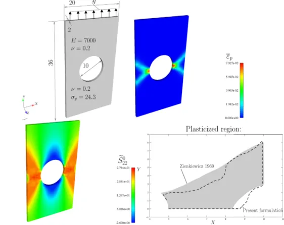
4.4. Drilled plate under tension
We now consider an elastic perfectly-plastic benchmark which was employed by Castellazzi, Artioli and Krysl [16] to validate their nodally integrated (element patch-based) NICE-T4 element. This is especially relevant, since their nodally integrated elements entail fewer degrees-of-freedom than the present element but produce denser Jacobian matrices. This can be observed inFig. 2in Ref. [16]. Krysl’s group ele-ments exhibit high performance in demanding problems, such as incom-pressible and bending-dominated problems. The problem is depicted in Fig. 9and agrees with the data reported in Ref. [16]. The data also cor-responds to the original problem by Zienkiewicz, Vallippan and King [52], who show results for the plastic region in the perfectly-plastic case. Contour plots for𝜀pand̃S022are shown, as well as a comparison of
the plasticized region near the hole are also shown inFig. 9. There are differences in the domain, when compared with the plot reported by Zienkiewicz, Vallippan and King. Both contour plots are very smooth, a consequence of the use of continuous stress interpolation. In terms
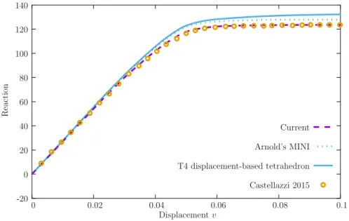
of reaction-displacement results, we compare our element and imple-mentation of MINI and T4 elements with that of Castellazzi, Artioli and Krysl. Two meshes are employed (respectively 142 elements and 2998 elements). We can observe in Fig. 10a that the new element perfor-mance for the coarse mesh is on-par with a much finer mesh by Castel-lazzi, Artioli and Krysl. Both MINI and T4 show stiffer results with the coarse mesh. Refining the mesh dilutes the advantage of our present formulation, however it still can be confirmed inFig. 10b.
5. Conclusions
By using the Hellinger-Reissner variational principle (cf [8]), we proposed a stress and displacement-based element for finite strains which can be viewed as an extension of the linear formulation by Dun-ham and Pister [20] for finite strains. A simple inf-sup numerical test is performed and an horizontal asymptote was obtained, indicating con-vergence for this formulation.
Compared with alternatives such as the stabilized nodal integra-tion [14,19,21,29,38] and smoothed edges [23,37] and faces [33], no densitification occurs (cf.Fig. 8of [21]) and the conventional imple-mentation is retained. In contrast with formulations based on bubbles [4,31,41], bending performance is greatly improved. Our formulation follows the traditional finite element assembling process, while excel-lent results are obtained in bending and incompressibility situations. Under this perspective, it is similar in approach to the nodal rotation technique by Nodargi et al. [35]. Computational cost is significant, but convergence curves show excellent behavior.
Compared with F formulations for hexahedra (cf [45]), crossed-mesh configurations typically outperform that formulation, even in
Fig. 10. Drilled plate under tension. Comparison with MINI, T4 and NICE-T4 elements for two distinct meshes.
bending-dominated situations. In addition, compared with hexahedra, tetrahedra have the advantage of being suitable for fracture problems and other non-smooth problems.
Appendix A. Supplementary data
Supplementary data to this article can be found online athttps:// doi.org/10.1016/j.finel.2019.07.003.
References
[1] N. Abboud, G. Scovazzi, Elastoplasticity with linear tetrahedral elements: a variational multiscale method, Int. J. Numer. Methods Eng. 115 (2018) 913–955. [2] P. Areias. Simplas.http://www.simplas-software.com. Portuguese Software
Association (ASSOFT) registry number 2281/D/17.
[3] P. Areias, T. Rabczuk, J.I. Barbosa, The extended unsymmetric frontal solution for multiple-point constraints, Eng. Comput. 31 (7) (2014) 1582–1607.
[4] P. Areias, Matou, Stabilized four-node tetrahedron with, Int. J. Numer. Methods Eng. 76 (2008) 1185–1201.
[5] P.M.A. Areias, J.M.A. Csar de S, C.A. Conceio Antnio, A.A. Fernandes, Analysis of 3D problems using a new enhanced strain hexahedral element, Int. J. Numer. Methods Eng. 58 (2003) 1637–1682.
[6] D.N. Arnold, F. Brezzi, M. Fortin, A stable finite element for the Stokes equations, Calcolo XXI (IV) (1984) 337–344.
[7] F. Auricchio, L. Beiro da Veiga, C. Lovadina, A. Reali, A stability study of some mixed finite elements for large deformation elasticity problems, Comput. Methods Appl. Math. 194 (2005) 1075–1092.
[8] K.-J. Bathe, Finite Element Procedures, Prentice-Hall, 1996.
[9] K.-J. Bathe, The inf-sup condition and its evaluation for mixed finite element methods, Comput. Struct. 79 (2001) 243–252.
[10] T. Belytschko, W.E. Bachrach, Efficient implementation of quadrilaterals with high coarse mesh accuracy, Comput. Methods Appl. Math. 54 (3) (1986) 279–301. [11] F. Brezzi, K.-J. Bathe, A discourse on the stability conditions for mixed finite
element formulations, Comput. Methods Appl. Mech. Eng. 82 (1990) 27–57. [12] F. Brezzi, M. Fortin, Mixed and Hybrid Finite Element Methods. Number 15 in
Springer Series in Computational Mathematics, Springer-Verlag, New York, 1991. [13] F. Brezzi, M. Fortin, Mixed and Hybrid Finite Element Methods. Number 15 in
Springer Series in Computational Mathematics, Springer, New York, 1991. [14] M. Broccardo, M. Micheloni, P. Krysl, Assumed-deformation gradient finite elements with nodal integration for nearly incompressible large deformation analysis, Int. J. Numer. Methods Eng. 78 (2009) 1113–1134.
[15]T.S. Cao, P. Montmitonnet, P.O. Bouchard, A detailed description of the Gurson-Tvergaard-Needleman model within a mixed velocity pressure finite element formulation, Int. J. Numer. Methods Eng. 96 (9) (2013) 561–583. [16]G. Castellazi, E. Artioli, P. Krysl, Linear tetrahedral element for problems of plastic
deformation, Meccanica 50 (2015) 3069–3086.
[17]I. Caylak, R. Mahnken, Stabilization of mixed tetrahedral elements at large deformations, Int. J. Numer. Methods Eng. 90 (2012) 218–242.
[18]D. Chapelle, K.-J. Bathe, The inf-sup test, Comput. Struct. 47 (1993) 537–545. [19]C.R. Dohrmann, M.W. Heinstein, J. Jung, S.W. Key, W.R. Witowski, Node-based
uniform strain elements for three-node triangular and four-node tetrahedral meshes, Int. J. Numer. Methods Eng. 47 (2000) 1549–1568.
[20]R.S. Dunham, K.S. Pister, A Finite Element Application of the Hellinger-Reissner Variational Theorem. Technical Report AFFDL-TR-68-150, vol. 45433, Air Force Flight Dynamics Laboratory, Wright Patterson AFB, OH, 1968.
[21]M.W. Gee, C.R. Dohrmann, S.W. Key, W.A. Wall, A uniform nodal strain tetrahedron with isochoric stabilization, Int. J. Numer. Methods Eng. 78 (2009) 429–443.
[22]S. Glaser, F. Armero, On the formulation of enhanced strain finite elements in finite deformations, Eng. Comput. 14 (7) (1997) 759–791.
[23]Z.C. He, G.Y. Li, Z.H. Zhong, A.G. Cheng, G.Y. Zhang, G.R. Liu, E. Li, Z. Zhou, An edge-based smoothed tetrahedron finite element method (es-t-fem) for 3d static and dynamic problems, Comput. Mech. 52 (2013) 221–236.
[24]E. Hellinger, Encyclopedia der Mathematishen Wissnschaften, ume 4, Teubner, Leipzig, 1914. chapter Die allgemeine Aussetze der Mechanik der Kontinua. [25]T.J.R. Hughes, The Finite Element Method. Dover Publications, 2000, Reprint of
Prentice-Hall edition, 1987.
[26]T.J.R. Hughes, L.P. Franca, M. Balestra, A new finite element formulation for computational fluid dynamics: V. circumventing the Babuska-Brezzi condition: a stable Petrov-Galerkin formulation of the Stokes problem accommodating equal-order interpolations, Comput. Methods Appl. Math. 59 (8599) (1986). [27]Y. Ko, K.-J. Bathe, Inf-sup testing of some three-dimensional low-order finite
elements for the analysis of solids, Comput. Struct. 209 (2018) 1–13. [28]J. Korelc, Multi-language and multi-environment generation of nonlinear finite
element codes, Eng. Comput. 18 (4) (2002) 312–327.
[29]P. Krysl, B. Zhu, Locking-free continuum displacement finite elements with nodal integration, Int. J. Numer. Methods Eng. 76 (2008) 1020–1043.
[30]I-Shih Liu, On the transformation property of the deformation gradient under a change of frame, J. Elast. 71 (1) (Apr 2003) 73–80.
[31]R. Mahnken, I. Caylak, G. Laschet, Two mixed finite element formulations with area bubble functions for tetrahedral elements, Comput. Methods Appl. Math. 197 (2008) 1147–1165.
[32]A. Masud, T.J. Truster, A framework for residual-based stabilization of incompressible finite elasticty: stabilized formulations
and$\overline{\boldsymbol{f}}$ methods for linear triangles and tetrahedra, Comput. Methods Appl. Math. 267 (2013) 359–399.
[33]T. Nguyen-Thoi, G.R. Liu, K.Y. Lam, G.Y. Zhang, A face-based smoothed finite element method (FS-FEM) for 3D linear and geometrically non-linear solid mechanics problems using 4-node tetrahedral elements, Int. J. Numer. Methods Eng. 78 (2009) 324–353.
[34]H. Nguyen-Xuan, G.R. Liu, An edge-based smoothed finite element method softened with a bubble function (bES-FEM) for solid mechanics problems, Comput. Struct. 128 (2013) 14–30.
[35] N.A. Nodargi, F. Caselli, E. Artioli, P. Bisegna, A mixed tetrahedral element with nodal rotations for large-displacement analysis of inelastic structures, Int. J. Numer. Methods Eng. 108 (2016) 722–749.
[36] T.H. Ong, C.E. Heaney, C.-K. Lee, G.R. Liu, H. Nguyen-Xuan, On stability, convergence and accuracy of bES-FEM and bFS-FEM for nearly incompressible elasticity, Comput. Methods Appl. Math. 285 (2015) 315–345.
[37] Y. Onishi, R. Lida, K. Amaya, F-bar aided edge-based smoothed finite element method using tetrahedral elements for finite deformation analysis of nearly incompressible solids, Int. J. Numer. Methods Eng. 109 (2017) 1582–1606. [38] M.A. Puso, J. Solberg, A stabilized nodeally integrated tetrahedral, Int. J. Numer.
Methods Eng. 67 (2006) 841–867.
[39] S. Reese, P. Wriggers, B.D. Reddy, A new locking-free brick element technique for large deformation problems in elasticity, Comput. Struct. 75 (2000) 291–304. [40] Wolfram Research Inc, Mathematica, 2007.
[41] I. Romero, M. Bischoff, Incompatible bubbles: a non-conforming finite element solution for linear elasticity, Comput. Methods Appl. Math. 196 (2007) 1662–1672.
[42] J.C. Simo, F. Armero, Geometrically non-linear enhanced strain mixed methods and the method of incompatible modes, Int. J. Numer. Methods Eng. 33 (1992) 1413–1449.
[43] J.C. Simo, F. Armero, R.L. Taylor, Improved versions of assumed strain tri-linear elements for 3D finite deformation problems, Comput. Methods Appl. Math. 110 (1993) 359–386.
[44] J.C. Simo, T.J.R. Hughes, Computational Inelasticity, corrected second printing edition, Springer, 2000.
[45] J.C. Simo, R.L. Taylor, K.S. Pister, Variational and projection methods for the volume constraint in finite deformation elasto-plasticity, Comput. Methods Appl. Math. 51 (1985) 177–208.
[46] R.L. Taylor, A mixed-enhanced formulation for tetrahedral finite elements, Int. J. Numer. Methods Eng. 47 (2000) 205–227.
[47] C. Truesdell, W. Noll, The Non-linear Field Theories of Mechanics, third ed., Springer, 2004.
[48] N. Viebahn, K. Steeger, J. Schrder, A simple and efficient Hellinger-Reissner type mixed finite element for nearly incompressible elasticity, Comput. Methods Appl. Math. 340 (2018) 278–295.
[49] E.L. Wilson, R.L. Taylor, W. P Doherty, J. Ghaboussi, Incompatible displacement models, in: S.J. Fenves, N. Perrone, A.R. Robinson, W.C. Schnobrich (Eds.), Numerical and Computer Models in Structural Mechanics, Academic Press, New York, 1973, pp. 43–57.
[50] X. Zeng, G. Scovazzi, N. Abboud, O. Coloms, S. Rossi, A dynamic variational multiscale method for viscoelasticity using linear tetrahedral elements, Int. J. Numer. Methods Eng. 112 (2016) 19512003.
[51] O.C. Zienkiewicz, R.L. Taylor, J.Z. Zhu, seventh ed., The Finite Element Method. Its Basics & Fundamentals, ume First, Butterworth-Heinemann, Elsevier, Oxford, OX5 1GB UK, 2013.
[52] O.C. Zienkiewicz, S. Vallippan, I.P. King, Elasto-plastic solutions of engineering problems. initial stress’, finite element approach, Int. J. Numer. Methods Eng. 1 (75100) (1969).