REM WORKING PAPER SERIES
The Impact of Hedge Fund indices on portfolio performance
Maria Teresa Medeiros Garcia, Gonçalo Liberal
REM Working Paper 085-2019
May 2019
REM – Research in Economics and Mathematics
Rua Miguel Lúpi 20, 1249-078 Lisboa,
Portugal
ISSN 2184-108X
Any opinions expressed are those of the authors and not those of REM. Short, up to two paragraphs can be cited provided that full credit is given to the authors.
1
The impact of hedge fund indices on portfolio performance
Maria Teresa Medeiros Garcia a,b,*, Gonçalo Liberala
a ISEG, Lisbon School of Economics and Management, Universidade de Lisboa, Portugal Rua Miguel Lupi, 20
1249-078 Lisboa, Portugal
b UECE (Research Unit on Complexity and Economics); REM –Research in Economics and Mathematics
Rua Miguel Lupi, 20 1249-078 Lisboa Portugal
UECE (Research Unit on Complexity and Economics) is financially supported by FCT (Fundação para a Ciência e a Tecnologia), Portugal. This article is part of the Strategic Project (UID/ECO/00436/2019).
* Correspondig author. Tel.: +351 21392599
E-mail addresses: [email protected] (M. T. M. Garcia), [email protected] (G. Liberal)
Abstract
The purpose of this paper is to assess the combination of investable hedge funds indices with a traditional portfolio of 60% stocks and 40% bonds. The S&P 500 Index, the Barclays US Aggregate Bond Index, and three investable hedge fund indices, the MEBI Maximum Sharpe Ratio L1 Index, the MEBI Zero Beta Strategy L1 Index, and the Eurekahedge ILS Advisers Index, were considered to conduct performance comparison, using time windows of two, five and ten years, from the 1st of January, 2006, to the 1st
2
of February, 2016. Significant reduction of the beta of the overall portfolio is reached. The findings showed that the investable hedge fund indices under analysis can be used as an easy way to protect a portfolio during different market conditions, diversifying the risks of the traditional investment portfolios. The paper provides evidence of how investable hedge fund indices lead to an improvement in the performance results, when compared with the traditional global equity-bond portfolio alone.
Keywords: Markowitz portfolio theory; optimal portfolios; investable hedge fund index; performance evaluation
Jel Classification: G11, G12
1. Introduction
For many years, in the 20th Century, institutional investors, such as public and private pension funds, as well as sovereign funds and insurance companies, have focused their allocation in a typical, simple, and diversified portfolio, composed of 60% equities and 40% bonds. This is the ideal asset allocation for the long-term investments of some private investors and balanced fund managers.
With this approach, also known as the 60-40 equity/fixed income portfolio, investors tend to follow a combination of global stocks and global bonds and expect to achieve improved risk-adjusted performance. This approach is used by passive investors for long-term growth. For example, index funds proved to be performance leaders with a low-cost
3
mutual structure and the indexing strategy (Bogle, 2014). If exchange-traded funds (ETF) are used, a new kind of index fund emerged late in the 20th Century, consisting of combining only two ETFs, with periodic rebalancing. Fund managers use this strategy actively as a benchmark in moderate or balanced mutual funds.
These portfolios have risk benefits, which allow for a broader exposure to equities, along with lower volatility provided by bonds, than 100% equity portfolios. Bonds also provide diversification benefits, due to the low correlation with stocks. This strategy is also used in all market conditions.
Although these portfolios have performed well during the 1980s and 1990s, with the passage to the 21st Century, fluctuating interest rates, a series of bear markets, and low interest rates have eroded the popularity of these portfolios. Given the current low interest rates and low bond yields, this asset class might increase its volatility, and thus contribute to an increased risk for these portfolios.
Therefore, it became necessary to increase exposure to other financial instruments in order to diversify these portfolios and reduce systemic risks in financial markets. One asset class that has grown its popularity is hedge funds and absolute return strategies which aim at better risk-adjusted performances. Both may present valid alternative investment in times of high volatility, and they have gained visibility in periods of bear markets, when compared to stock index funds, which has consequently led to an increase of assets under management for this kind of assets.
4
This study introduces hedge fund strategies or absolute return strategies allocation into a simple 60-40 equity/fixed income portfolio, in order to measure their performance on the overall portfolio. We compare the performance of a passive index portfolio of 60% global equity and 40% global fixed income, with the allocation of hedge funds strategies in the main portfolio.
The objective is to show that the performance of a simple portfolio can be improved when combined with hedge funds indices, thus illustrating that an investable hedge fund index can be an easy way to protect a conservative or balanced portfolio and to minimize its volatility, whilst increasing the return and provide a decreasing exposure to the market. Successful and accessible absolute return strategies are presented in different timeframes.
The paper is organised as follows. The next section provides a framework for the construction of portfolios and hedge fund investment strategies. In Section 3, the data and methodology are presented. Section 4 shows the empirical results, and Section 5 concludes.
2. Framework
In his seminal papers, Markowitz (1952) introduced the Modern Portfolio Theory (MPT) showing the importance of diversification and the effects of covariance of assets returns in the choice of the optimal portfolio. Selecting securities with lower covariances reduce portfolio volatility, or risk. Investors should select their portfolios based upon the
5
expected return and the variance of return of each asset and also determine asset weights, resulting in the overall risk-reward of the portfolio, thus minimising the risk given a
certain rate of return.
This leads to the representation of the efficient frontier, where each level of expected return has the minimum level of volatility, and each level of volatility has the higher expected return. The minimum variance portfolio is the combination of higher-risk assets that has the lowest possible variance, i.e., it is the efficient portfolio with lower risk (Bodie
et al., 2011). The Markowitz portfolio is the combination of assets that maximizes the
relation between risk and return, i.e., the maximization of the Sharpe ratio (1966). The selection of the optimal portfolio should be made along the efficient frontier, in an attempt to reach all investors’ profiles (Edwin & Gruber, 2011). The optimal portfolio selection is the efficient portfolio which maximizes the utility function of the investor, i.e., with the greatest expected utility from the investors’ perspective.
The MPT focused on the construction of portfolios with two asset classes: stocks and bonds. In the 1950s, these asset classes were used to build a well-diversified portfolio. Markowitz (1952a) used the classical market-capitalization-weighted portfolio, whereas the 60/40 ratio of stocks and bonds represented the global universe of investable markets. He concluded that this combination provides the maximum return for a given amount of risk. This asset class blend has become the reference for a moderate or balanced portfolio
6
over the last decades. Historically, this portfolio allocation has been shown to offer solid returns, with a moderate risk profile over the long-term (Bernstein, 2002).
Implicit to this strategy, besides the diversification factor, is the low correlation between bonds and stocks. When combined and moving differently, these two asset classes can smooth out volatility, resulting in a diversified portfolio that should be less volatile, with less severe losses than in a 100% equity portfolio.
The overall risk and return of the 60/40 portfolio varies greatly, and the volatility and risk premium of equities has changed since Markowitz presented his theory. The 60/40 portfolio in today’s market has more risk than the same allocation portfolio of decades earlier. The correlation between stocks and bonds is increasing, and low interest rates are associated with low bond yields and increasing volatility in bonds, as shown in the two-factor model of Fong and Vasicek (1991). When interest rates rise, bond prices tend to fall (Martellini et al., 2003), and the downside protection from bonds allocation tends to fail in periods when there is high volatility in stock market (Schwert, 1989). The equity market fall of 40% in 2008 challenged the efficacy of the 60/40 portfolio, and proved that this portfolio was not properly diversified.
Today’s investors and fund managers desire a smoother ride and better downside protection. For this purpose, investors or institutional portfolios search for tools to customise portfolios and improve their performance in terms of risk-adjusted returns, volatility, diversification, correlation and downside protection. In order to beat their
7
performance, investors combine other investment vehicles, including hedge funds or absolute return funds indices.
The term hedge fund is commonly used to describe an alternative investment that has the goal of generating improved risk-adjusted performance or absolute returns. Many hedge funds are not actually hedged at all, and they often take large risks on speculative strategies in order to achieve performance returns, irrespective of which way the markets are heading.
According to Anson (2006), the term hedge fund was first applied in 1949, by Alfred Jones to his private investment fund, which combined the simultaneous use of long and short equity positions to hedge the portfolio's exposure to movements in the market (Purcell et al., 1999). This strategy is known as Long Short Equity, and is the most common-used in hedge funds today (McCrary, 2005).
Nowadays, hedge funds often do not really hedge market risk, and Alfred Jone’s definition is not precise. For Ackermann (1999), hedge funds began as investment partnerships that could take long and short positions. However, they have evolved into a multifaceted organisational structure that defies simple definition. Therefore, the author characterises hedge funds by a set of features, namely: a largely unregulated organisational structure; flexible investment strategies; relatively sophisticated investors; substantial managerial investment, and; strong managerial incentives. Hedge funds can therefore yield insight into the impact of regulation, alternative investment practices, and
8
incentive alignment on performance. According to Jaeger (2003), a hedge fund is an actively-managed investment fund which seeks an attractive absolute return, using a wide variety of investment strategies and tools.
Nowadays, the Hedge Fund Marketing Association has adopted the following definition: “A hedge fund is an alternative investment that is designed to protect
investment portfolios from market uncertainty, while generating positive returns in both up and down markets. Throughout time investors have looked for ways to maximize profits while minimizing risk. The issue of shielding an investment from market risk is attempted (although not always successful) with alternative investments that try to mitigate loss and preserve capital. “
The idea of a defensive instrument, designed to protect portfolios is underlying, and will be used throughout the paper.
As hedge funds often have high minimum investments, these instruments are only accessible to institutional investors and very wealthy private investors, or billionaires who can afford them. However, some Mutual Funds and UCITS1 exclusively invest in absolute
1 “UCITS” or “undertakings for the collective investment in transferable securities” are investment funds
regulated at the European Union level. They account for around 75% of all collective investments by small investors in Europe. The legislative instrument covering these funds is Directive 2014/91/EU. Source: European Commission Website.
9
return strategies with low minimum investments, which are accessible to all types of investors.
Although this type of financial instruments is considered complex, it has grown in popularity, resulting in an increasing upwards trend of assets under management (AUM), up until the present day. Figure 1 shows the increase of AUM for the hedge funds industry between 1997 and 2016.
Figure 1. Historical Growth of Assets under Management for the Hedge Fund industry, 1997 - 2016 Source: http://www.barclayhedge.com/
Hedge funds can be open or closed funds, and their managers can invest in a diverse range of markets, employing a wide variety of financial instruments2 and risk management techniques, which can be divided into investment strategies.
10
The most common hedge fund investment strategies are divided into: relative value and directional. According to Ackermann (1999) and Credit Suisse Hedge Fund Index rules, the component investment strategies that comprise the eleven style-based sectors are based on the following hedge fund investment strategies:
Convertible Arbitrage: funds that aim to profit from the purchase of convertible securities
and the subsequent shorting of the underlying stock when there is a pricing discrepancy made in the conversion factor of the security.
Fixed Income Arbitrage: generates profits by exploiting inefficiencies and price
anomalies between related fixed income securities. This strategy may include leveraging long and short positions in fixed income securities, and trading techniques involving interest rate swaps, government securities, and futures;
Dedicated Short Bias: funds which take shorter, rather than long positions and which earn
returns by maintaining net short exposure in long and short equities.
Equity Market Neutral: is when the manager takes both long and short positions in stocks,
whilst attempting to lock-out, or neutralize market risk. (i.e., a beta of zero is desired). Managers often apply leverage to enhance returns.
Event Driven: occurs when the manager invests in various asset classes and seeks to profit
from potential mispricing of securities that are related to a specific corporate or market event3. These funds can invest in equities, fixed income instruments (investment grade,
3 Mergers, bankruptcies, financial or operational stress, restructurings, asset sales, recapitalizations,
11
high yield, bank debt, convertible debt and distressed), options, and various other derivatives. The common subcategories in Event Driven strategies are: Risk Arbitrage and Distressed Securities.
Risk Arbitrage: is when the manager attempts to capture the spreads in merger or
acquisition transactions involving public companies, after the terms of the transaction have been announced. A risk arbitrager typically buys the stock of the company being acquired and simultaneously shorts the acquirer’s stock, according to the merger ratio.
The principal risk is deal risk, should the deal fail to close.
Distressed Securities: in this case, the manager focuses on companies which are suffering
financial/operational distress or bankruptcy proceedings. Such securities trade at substantial discounts to their intrinsic value, due to difficulties in assessing their proper value. This strategy is generally long-biased in nature, whereby the manager attempts to profit from the issuer’s ability to improve its operation, but may take short positions when
a successful outcome to the bankruptcy process is expected, which ultimately leads to an exit strategy.
Global Macro: is when managers carry long and short positions in the global markets.
Their positions reflect their views on overall market directions, as influenced by economic trends, events, or changes in interest rates. Global Macro fund portfolios can include stocks, bonds, currencies, commodities, and derivatives instruments. Managers also use leverage, and most funds invest globally in both developed and emerging markets. Profits
12
are made by correctly anticipating price movements in global markets and by having the flexibility to manage portfolio instruments.
Long/Short Equity: funds invest on both long and short sides of equity markets, generally focusing on diversifying or hedging across particular sectors, regions, or market capitalisations. The use of leverage is common in their portfolios.
Managed Futures or Commodity Trading Advisors (CTA): focus on investing in listed
financial and commodity futures markets and currency markets around the world. Managers tend to employ systematic trading programmes that largely rely upon historical price data and market trends. In this case, a significant amount of leverage is employed, as the strategy involves the use of futures contracts.
Multi-Strategy: occurs when managers allocate capital based on perceived opportunities
among several hedge fund strategies. Through the diversification of capital, managers seek to consistently deliver positive returns, regardless of the directional movement of markets. The added diversification benefits reduce the risk profile and help smooth returns, reduce volatility and decrease asset-class and single-strategy risks.
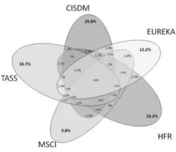
The hedge fund databases do not cover the whole of the hedge fund industry. Therefore, the hedge fund indices are not representative of the total hedge fund universe (Agarwal et al, 2013). The five major hedge fund databases are: CISDM, HFR, Eureka, MSCI, and, TASS. They represent the most comprehensive hedge funds database that has been used in the literature. According to Agarwal et al. (2013), less than one percent of
13
the hedge fund industry reported to the databases referred to above in 2009, as represented in Figure 2.
Figure 2. Venn diagram of the 5 major Hedge Funds databases, where the percentage of funds covered by each database is represented individually, and also by all the possible combinations of multiple databases Source: Agarwal et al. (2013)
The hedge fund database provider aggregates several funds which have reported performance and then constructs indices itself. The hedge fund indices can be strategy-specific, asset-weighted, equally-weighted, investable, or non-investable.
In order to represent the hedge fund universe and to overcome the performance biases that were identified by Brown (1999) and Fung and Hsieh (2000), we only use investable hedge fund indices. In addition, investable indices are unaffected by survivorship or backfilling biases (Heidorn et al., 2010; Park, 1999). Further, ‘Investable’ means that the
14
constituents of the index are open to investment, and are not necessarily investing in the main index, as to have any impact on the overall portfolio, Amin and Kat (2003) show that allocations to hedge funds would have to far exceed the typical 1% to 5% that many institutions typically consider.
. This means that we cannot directly invest in the indices themselves. Investing in a hedge fund index is achieved via proxy products known as trackers, which replicate an index performance. We selected a hedge fund database with investable indexes, where investment is available by a tracker.
3. Data and Methodology
3.1 Data
The 60/40 portfolio represents a passively managed index portfolio, consisting of 60% from the S&P 500 Index4 and 40% from the Barclays US Aggregate Bond Index5. The historical data of the S&P 500 Index and the Barclays US Aggregate Bond Index were taken from the Datastream platform, from the 1st of January, 2006, to the 1st of February, 2016. An initial investment of $100,000 in January 2006 was considered.
4 The Standard & Poor's 500 Index is a capitalization-weighted index of 500 stocks. The index is designed
to measure performance of the broad domestic economy through changes in the aggregate market value of 500 stocks representing all major industries.
5 The index measures the performance of the U.S. investment grade bond market. The index invests in a wide spectrum of public, investment-grade, taxable, fixed income securities in the United States – including government, corporate, and international dollar-denominated bonds, as well as mortgage-backed and asset-backed securities, all with maturities of more than 1 year. Source: http://etfdb.com/
15
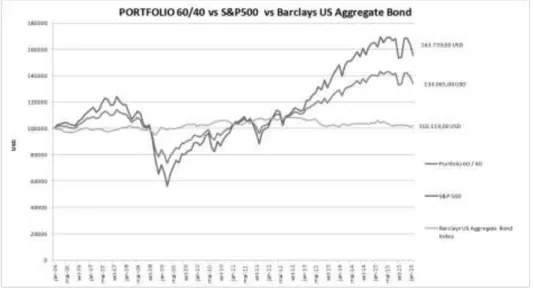
We focused on static portfolios, with no rebalancing (weights do not change). Figure 3 displays the historical evolution of a $100,000 investment in the traditional portfolio.
Figure 3. Historical evolution of 60/40 portfolio, the S&P 500 and the Barclays US Aggregate Bond, between 1st January, 2006 and 31st January, 2016
We computed the holding period returns, the annual returns, and standard deviations of the 60/40 portfolio (Table 1).
Table 1. Risk and Return of the 60/40 portfolio, 2006 - 2016 Portfolio 60 / 40 10 Years 5 Years 2 Years Holding period return 38.70% 35.36% 7.24% Average annual return 3.33% 6.24% 3.56% Risk (standard deviation) 10.39% 8.51% 9.01%
For hedge fund indices, we used data from the www.eurekahedge.com website. To select the eligible indices, we used the two following requirements: 1) historical data from
16
the last 10 years, from the first month of 2006 through to the first month of 2016, and; 2) an index composed of liquid investable hedge funds, tracked by an investable fund which replicates index performance.
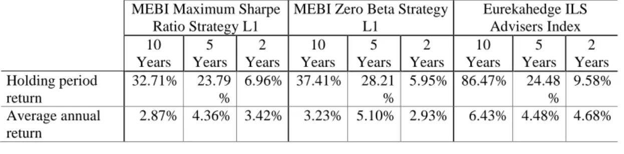
Accordingly, the three selected hedge fund indices, which were denominated as HF1, HF2 and HF3, were the following:
HF1: MEBI Maximum Sharpe Ratio L1 Index - The MEBI Maximum Sharpe Ratio L1 is a Mizuho-Eurekahedge Bespoke index, which aims to maximize the expected Sharpe ratio under pre-determined assumptions, with its 4 constituent assets being: Japanese bonds, US bonds, Japanese equities, and US equities. The index is updated on a daily basis on working days in Tokyo and Singapore.
HF2: MEBI Zero Beta Strategy L1 Index - The MEBI Zero Beta Strategy L1 is a Mizuho-Eurekahedge Bespoke index which aims to have zero correlation for Japanese bonds under pre-determined assumptions, with its 4 constituent assets being: Japanese bonds, US bonds, Japanese equities and US equities. The index is updated on a daily basis on working days in Tokyo and Singapore.
HF3: Eurekahedge ILS Advisers Index - The Eurekahedge ILS Advisers Index is ILS Advisers and Eurekahedge’s collaborative equally weighted index of 32 constituent funds. The index is designed to provide a broad measure of the performance of those underlying hedge fund managers who explicitly allocate insurance linked investments and have at least 70% of their portfolio invested in non-life risk. The index was base-weighted at 100 for December 2005, and does not contain duplicate funds, being denominated in local currencies.
We computed the holding period returns, the annual returns, and the standard deviations for each hedge fund index (Table 2).
Table 2. Risk and Return of the HF1, HF2, and HF3 Hedge Fund strategies, 2006 - 2016
MEBI Maximum Sharpe Ratio Strategy L1
MEBI Zero Beta Strategy L1 Eurekahedge ILS Advisers Index 10 Years 5 Years 2 Years 10 Years 5 Years 2 Years 10 Years 5 Years 2 Years Holding period return 32.71% 23.79 % 6.96% 37.41% 28.21 % 5.95% 86.47% 24.48 % 9.58% Average annual return 2.87% 4.36% 3.42% 3.23% 5.10% 2.93% 6.43% 4.48% 4.68%
17
Risk (standard deviation)
3.13% 2.49% 2.61% 5.53% 4.93% 6.20% 2.08% 2.28% 0.91%
3.2 Methodology
The combinations of the traditional 60/40 portfolio with each of the three selected hedge fund indices were implemented in order to select the correspondent minimum variance and the Markowitz portfolios. Short selling (or short positions) was restricted, as it is not accessible to individual investors, and because most institutional investors do not short sell, given that the practice is forbidden by law in many institutions (Elton et al., 2010).
For the optimal portfolios, several well-known measures of performance were obtained, such as: Beta, Sharpe Ratio, Treynor Ratio, Jensen’s Alpha, and Information Ratio. The Beta measures systematic risk. Investors prefer portfolios with higher Sharpe Ratios (Sharpe, 1966; Bodie et al., 2011), and the higher the Treynor ratio, the better the performance of the portfolio under analysis. This ratio is recommended for evaluating well-diversified portfolios which produce the excess returns that could have been earned on an investment that has no diversifiable risk (Treynor and Black, 1973).
Jensen’s Alpha measures the average excess return on the portfolio in relation to that
predicted by the capital asset pricing model (CAPM), for a given portfolio’s beta and the average market return (Jensen, 1968). A positive Alpha is a sign that a portfolio outperformed the market, whilst a negative value indicates underperformance. The higher the alpha, the more a portfolio has earned above the level predicted.
18
Finally, the information ratio (IR) divides the alpha of the portfolio by the tracking error, measured by the standard deviation of the difference between the returns of the portfolio and its benchmark. It measures the excess return per unit of non-systematic risk of the portfolio, or the risk that could be diminished by holding a market index portfolio. The IR is used for measuring active managers against a passive benchmark. This parameter is often used to evaluate mutual funds and hedge funds, as the IR shows the consistency of the fund manager in generating superior risk adjusted performance. A higher IR shows that the manager has outperformed other fund managers and has delivered consistent returns over a specified period of time (Goodwin, 1998).
As there is no theoretic unanimity concerning what the optimal evaluation period should be, we adopted both a ten and a five years period to conduct our analysis.
These measures of performance were assessed for the benchmark portfolio and for the optimal portfolio. We expect the benchmark portfolio to be lowly correlated with the hedge fund index. Therefore, it is expected that the variability of the overall portfolio or optimal portfolio will decrease, and that the performance measures increase.
4. Results
Firstly, the analysis assesses the impact of combining the traditional 60/40 portfolio with each hedge fund index on the return and volatility of the portfolios, based on returns between January 2006 and February 2016. We started to increase the weight of each
19
hedge fund index in the traditional 60/40 equity-bond portfolio, in order to assess the volatility, the return, and the Sharpe ratio of the combined portfolio.
This procedure allows us to obtain the minimum variance portfolios.
Tables 3.A, 3.B and 3.C present the results for different combinations of the traditional 60/40 equity bond portfolio and the MEBI Maximum Sharpe Ratio Strategy L1, the MEBI Zero Beta Strategy L1, and the Eurekahedge ILS Advisers Index (weightings from 0% to 100%).
Table 3.A. Volatility, expected return and Sharpe ratio of the combination portfolio with HF1 - MEBI Maximum Sharpe Ratio Strategy L1 index and the 60/40 portfolio
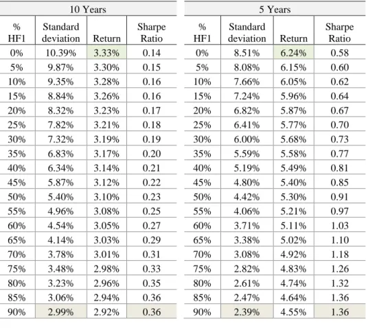
10 Years 5 Years % HF1 Standard deviation Return Sharpe Ratio % HF1 Standard deviation Return Sharpe Ratio 0% 10.39% 3.33% 0.14 0% 8.51% 6.24% 0.58 5% 9.87% 3.30% 0.15 5% 8.08% 6.15% 0.60 10% 9.35% 3.28% 0.16 10% 7.66% 6.05% 0.62 15% 8.84% 3.26% 0.16 15% 7.24% 5.96% 0.64 20% 8.32% 3.23% 0.17 20% 6.82% 5.87% 0.67 25% 7.82% 3.21% 0.18 25% 6.41% 5.77% 0.70 30% 7.32% 3.19% 0.19 30% 6.00% 5.68% 0.73 35% 6.83% 3.17% 0.20 35% 5.59% 5.58% 0.77 40% 6.34% 3.14% 0.21 40% 5.19% 5.49% 0.81 45% 5.87% 3.12% 0.22 45% 4.80% 5.40% 0.85 50% 5.40% 3.10% 0.23 50% 4.42% 5.30% 0.91 55% 4.96% 3.08% 0.25 55% 4.06% 5.21% 0.97 60% 4.54% 3.05% 0.27 60% 3.71% 5.11% 1.03 65% 4.14% 3.03% 0.29 65% 3.38% 5.02% 1.10 70% 3.78% 3.01% 0.31 70% 3.08% 4.92% 1.18 75% 3.48% 2.98% 0.33 75% 2.82% 4.83% 1.26 80% 3.23% 2.96% 0.35 80% 2.61% 4.74% 1.32 85% 3.06% 2.94% 0.36 85% 2.47% 4.64% 1.36 90% 2.99% 2.92% 0.36 90% 2.39% 4.55% 1.36
20
95% 3.01% 2.89% 0.35 95% 2.40% 4.45% 1.32 100% 3.13% 2.87% 0.33 100% 2.49% 4.36% 1.23
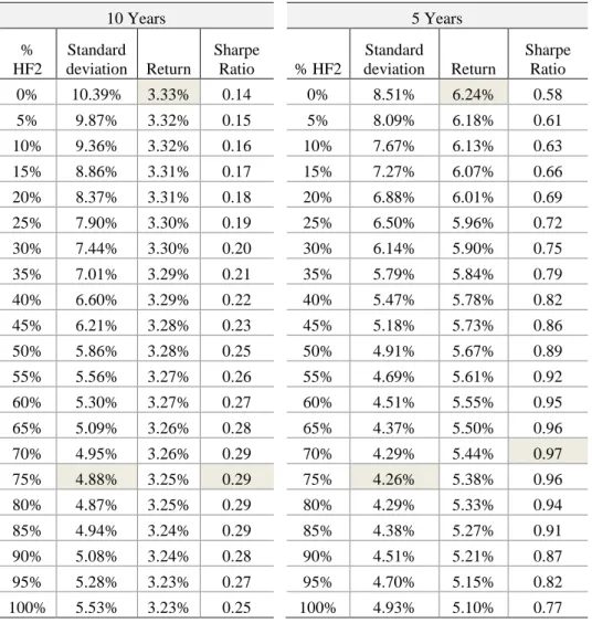
Table 3.B. Volatility, expected return and Sharpe ratio of the combination portfolio with HF2 - MEBI Zero Beta Strategy L1 index and the 60/40 portfolio
10 Years 5 Years % HF2 Standard deviation Return Sharpe Ratio % HF2 Standard deviation Return Sharpe Ratio 0% 10.39% 3.33% 0.14 0% 8.51% 6.24% 0.58 5% 9.87% 3.32% 0.15 5% 8.09% 6.18% 0.61 10% 9.36% 3.32% 0.16 10% 7.67% 6.13% 0.63 15% 8.86% 3.31% 0.17 15% 7.27% 6.07% 0.66 20% 8.37% 3.31% 0.18 20% 6.88% 6.01% 0.69 25% 7.90% 3.30% 0.19 25% 6.50% 5.96% 0.72 30% 7.44% 3.30% 0.20 30% 6.14% 5.90% 0.75 35% 7.01% 3.29% 0.21 35% 5.79% 5.84% 0.79 40% 6.60% 3.29% 0.22 40% 5.47% 5.78% 0.82 45% 6.21% 3.28% 0.23 45% 5.18% 5.73% 0.86 50% 5.86% 3.28% 0.25 50% 4.91% 5.67% 0.89 55% 5.56% 3.27% 0.26 55% 4.69% 5.61% 0.92 60% 5.30% 3.27% 0.27 60% 4.51% 5.55% 0.95 65% 5.09% 3.26% 0.28 65% 4.37% 5.50% 0.96 70% 4.95% 3.26% 0.29 70% 4.29% 5.44% 0.97 75% 4.88% 3.25% 0.29 75% 4.26% 5.38% 0.96 80% 4.87% 3.25% 0.29 80% 4.29% 5.33% 0.94 85% 4.94% 3.24% 0.29 85% 4.38% 5.27% 0.91 90% 5.08% 3.24% 0.28 90% 4.51% 5.21% 0.87 95% 5.28% 3.23% 0.27 95% 4.70% 5.15% 0.82 100% 5.53% 3.23% 0.25 100% 4.93% 5.10% 0.77
Table 3.A shows that an increasing weight of the MEBI Maximum Sharpe Ratio Strategy, decreases the annual variability. The optimal combination of this strategy is
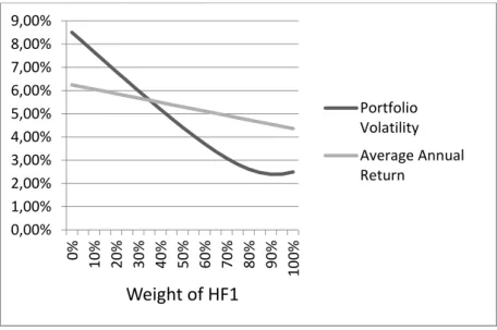
21
91% of HF1 for the 10 year period, reaching a minim volatility of 2.99%. For a five year period, the weight is 92%, as shown in Figures 4.A1 and 4.A2, which illustrate the consistent optimal allocation for this hedge fund strategy.
Table 3.C. Volatility, expected return and Sharpe ratio of the combination portfolio with HF3 - MEBI Eurekahedge ILS Advisers Index and the 60/40 portfolio
10 Years 5 Years % HF3 Standard deviation Return Sharpe Ratio % HF3 Standard deviation Return Sharpe Ratio 0% 10.39% 3.33% 0.14 0% 8.51% 6.24% 0.58 5% 9.87% 3.48% 0.17 5% 8.08% 6.15% 0.60 10% 9.35% 3.64% 0.19 10% 7.66% 6.07% 0.62 15% 8.84% 3.79% 0.22 15% 7.24% 5.98% 0.65 20% 8.32% 3.95% 0.25 20% 6.82% 5.89% 0.67 25% 7.81% 4.10% 0.29 25% 6.40% 5.80% 0.70 30% 7.30% 4.26% 0.33 30% 5.99% 5.71% 0.74 35% 6.80% 4.41% 0.38 35% 5.58% 5.62% 0.78 40% 6.29% 4.57% 0.43 40% 5.18% 5.54% 0.82 45% 5.79% 4.72% 0.50 45% 4.78% 5.45% 0.87 50% 5.30% 4.88% 0.57 50% 4.40% 5.36% 0.93 55% 4.82% 5.03% 0.66 55% 4.02% 5.27% 0.99 60% 4.35% 5.19% 0.77 60% 3.66% 5.18% 1.06 65% 3.89% 5.34% 0.90 65% 3.32% 5.09% 1.15 70% 3.45% 5.50% 1.06 70% 3.00% 5.01% 1.24 75% 3.04% 5.65% 1.26 75% 2.72% 4.92% 1.33 80% 2.67% 5.81% 1.49 80% 2.49% 4.83% 1.42 85% 2.37% 5.96% 1.75 85% 2.31% 4.74% 1.49 90% 2.15% 6.12% 1.99 90% 2.22% 4.65% 1.52 95% 2.05% 6.27% 2.17 95% 2.21% 4.56% 1.48 100% 2.08% 6.43% 2.21 100% 2.28% 4.48% 1.40
22
Figure 4.A1. Volatility and average annual return of the combination portfolio with HF1 and the 60/40 portfolio, during the ten year period
Figure 4.A2. Volatility and average annual return of the combination portfolio with HF1 and the 60/40 portfolio, during the five year period
0,00% 1,00% 2,00% 3,00% 4,00% 5,00% 6,00% 7,00% 8,00% 9,00% 0% 10% 20% 30% 40% 50% 60% 70% 80% 90% 10 0% Weight of HF1 Portfolio Volatility Average Annual Return 0,00% 2,00% 4,00% 6,00% 8,00% 10,00% 12,00% 0% 10% 20% 30% 40% 50% 60% 70% 80% 90% 10 0% Weight of HF1 Portfolio Volatility Average Annual Return
23
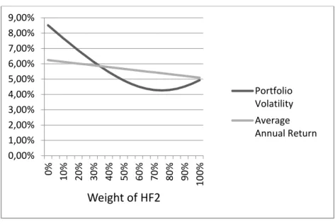
For the MEBI Zero Beta Strategy L1, we can see that the optimal allocation, for the ten year period, is 78%, and for the five year period, it is 75% (Table 3.B and Figures 4.B1 and 4.B2).
Figure 4.B1. Volatility and average annual return of the combination portfolio with HF2 and the 60/40 portfolio, during the ten year period
0,00% 2,00% 4,00% 6,00% 8,00% 10,00% 12,00% 0% 10% 20% 30% 40% 50% 60% 70% 80% 90% 10 0% Weight of HF2 Portfolio Volatility Average Annual Return
24
Figure 4.B2. Volatility and average annual return of the combination portfolio with HF2 and the 60/40 portfolio, during the five year period
Regarding the third strategy, the Eurekahedge ILS Advisers Index, the optimal allocation is obtained with a weight of 96%, for the ten year period, and of 93% for the five year period (Table 3.C and Figures 4.C1and 4.C2).
0,00% 1,00% 2,00% 3,00% 4,00% 5,00% 6,00% 7,00% 8,00% 9,00% 0% 10% 20% 30% 40% 50% 60% 70% 80% 90% 10 0% Weight of HF2 Portfolio Volatility Average Annual Return
25
Figure 4.C1. Volatility and average annual return of the combination portfolio with HF3 and the 60/40 portfolio, during the ten year period
Figure 4.C2. Volatility and average annual return of the combination portfolio with HF3 and the 60/40 portfolio, during the five year period
0,00% 2,00% 4,00% 6,00% 8,00% 10,00% 12,00% Weight of HF3 Portfolio Volatility Average Annual Return 0,00% 1,00% 2,00% 3,00% 4,00% 5,00% 6,00% 7,00% 8,00% 9,00% 0% 10% 20% 30% 40% 50% 60% 70% 80% 90% 10 0% Weight of HF3 Portfolio Volatility Average Annual Return
26
Table 4 synthetizes the weights to reach the combined portfolios with minimum volatility.
Table 4. Optimal weights Minimum variance portfolio
H1 H2 H3 10 years 91% 78% 96% 5 years 92% 75% 93% Markowitz portfolio H1 H2 H3 10 years 88% 77% 99%
To obtain the Markowitz portfolios, we assessed the Sharpe ratio of the combined portfolio. As we can observe in Figure 5.A, the Sharpe ratio of the portfolio increases the higher the weight of HF1 is. The maximum Sharpe ratio has been reached with a weight of 88% of HF1, considering the ten year period. In regards with the combination with HF2, the optimal weight is 77%, and with HF3, the optimal weight is 99% (Figures 5.B and 5.C).
27
Figure 5.A. Sharpe ratio of portfolios for different weights of HF1 and the traditional 60/40 portfolio during the ten year period
Figure 5.B. Sharpe ratio of portfolio for different weights of HF2 and the traditional 60/40 portfolio during the ten year period
0,00 0,05 0,10 0,15 0,20 0,25 0,30 0,35 0,40 0% 5% 10% 15% 20% %25 30% 35% 40% 45% %50 55% 60% 65% 70% 75% 80% 85% 90% 95% 10 0% Weight of HF1 0,00 0,05 0,10 0,15 0,20 0,25 0,30 0,35 0% 5% 10% 15% 20% %25 30% 35% 40% 45% %50 55% 60% 65% 70% 75% 80% 85% 90% 95% 10 0% Weight of HF2
28
Figure 5.C. Sharpe ratio of portfolio for different weights of HF3 and the traditional 60/40 portfolio during the ten year period
Naturally, the minimum variance portfolios show similar weights when compared with Markowitz portfolios. Therefore, the following strategies using a hedge fund index were selected to be analysed and labelled optimal portfolios:
Portfolio A: 90% for HF1 and 10% for 60/40 portfolio; Portfolio B: 75% for HF2 and 25% for 60/40 portfolio; Portfolio C: 95% for HF3 and 5% for 60/40 portfolio.
We can also represent the efficient frontier for each hedge fund combination with the traditional equity-bond, where each level of expected return has the minimum level of volatility. The graphical representations of the efficient frontier can be observed in Figure 6.A, Figure 6.B, and Figure 6.C, referring to HF1, HF2 and HF3, respectively.
0,00 0,50 1,00 1,50 2,00 2,50 0% 5% 10% 15% 20% %25 30% 35% 40% 45% %50 55% 60% 65% 70% 75% 80% 85% 90% 95% 10 0% Weight of HF3
29
Figure 6.A. Efficient frontier combining HF1 with the traditional 60/40 portfolio during the ten year period
Figure 6.B. Efficient Frontier combining HF2 with the traditional 60/40 portfolio during the ten year period 2,80% 2,90% 3,00% 3,10% 3,20% 3,30% 3,40% 0,00% 2,00% 4,00% 6,00% 8,00% 10,00% 12,00% R e tu rn Standard Deviation 3,00% 3,05% 3,10% 3,15% 3,20% 3,25% 3,30% 3,35% 0,00% 2,00% 4,00% 6,00% 8,00% 10,00% 12,00% R e tu rn Standard Deviation
30
Figure 6.C. Efficient Frontier combining HF3 with the traditional 60/40 portfolio during the ten year period
We further performed a backtest with the optimal hedge fund allocation previously-presented for each strategy and assessed the performance measures for each portfolio. We considered the period between January 2006 and February 2016, referring to the ten, five and two last year’s periods. We then compared our three portfolios (A, B, and C) with the
benchmark portfolio - the 60/40 global equity-bond portfolio - for the same periods.
Table 5.A presents performance indicators for the A portfolio. The average annual return decreases slightly during the three different periods, and the portfolio volatility significantly decreased from 10.39% to 2.85% during the ten year period, and from 8.51% to 2.31% during the five year period. For the two year period, we register a decrease from 9.01% to 2.40% in the variability of the portfolio, resulting in a lower risk for the
3,00% 3,50% 4,00% 4,50% 5,00% 5,50% 6,00% 6,50% 7,00% 0,00% 2,00% 4,00% 6,00% 8,00% 10,00% R e tu rn Standard Deviation
31
portfolio. Consequently, the Sharpe ratio of the portfolio increases with all time periods under analysis, meaning that the portfolio achieved better risk-adjusted returns.
Table 5.A. Risk and performance indicators for the 60/40 portfolio and Portfolio A for the ten, five and two year periods
The portfolio beta decreases from 0.57 to 0.03 during the ten year period, reflecting a very low risk exposure or sensitivity to the market. For the five and two year periods, the portfolio beta was consistent with the ten year period. The Treynor ratio significantly increases in all time periods, which indicates a better performance of the portfolio under study. Jensen alpha was positive, thus reflecting that the portfolio performed better when compared to its benchmark during the three time periods in analysis.The tracking error was higher, meaning that there are significant differences between the returns of the portfolio and its benchmark. The high Information Ratio shows that the portfolio has outperformed its benchmark and has delivered consistent returns over the period of time under analysis.
10 Years 5 Years 2 Years 10 Years 5 Years 2 Years Absolute Performance Rp 38.70% 35.36% 7.24% 33.31% 24.90% 6.99%
Average Annual Return Rp 1A 3.33% 6.24% 3.56% 2.92% 4.55% 3.43%
Portfolio Volatility σ 10.39% 8.51% 9.01% 2.85% 2.31% 2.40% Portfolio Beta β 0.57 0.60 0.68 0.03 0.05 0.05 Sharpe Index IS 0.14 0.58 0.31 0.38 1.41 1.10 Treynor Index T 0.03 0.08 0.04 0.42 0.71 0.54 Jensen's Alpha J 0.05% -0.54% -0.83% 1.02% 2.84% 2.39% Tracking Error TE 10.26% 8.21% 8.68% Information Ratio IR 0.10 0.35 0.28
32
Table 5.B presents performance indicators for portfolio B, with a 75% weight in the MEBI MEBI Zero Beta Strategy L1 index, and a 25% weight of the traditional 60/40 portfolio. The average annual return decreases slightly in all time periods, and the portfolio volatility significantly decreased from 10.39% to 4.66% during the ten year period, from 8.51% to 4.22 % during the five year period, and from 9.01% to 5.25% during the two year period, which results in a lower risk for the portfolio. Consequently, the Sharpe ratio of the portfolio increases during every time period under analysis, which means that this portfolio achieved better risk-adjusted returns.
Table 5.B. Risk and performance indicators for the 60/40 portfolio and Portfolio B for the ten, five and two year periods
The portfolio beta portfolio decreases from 0.57 to 0.10 during the ten year period, reflecting a very low risk exposure or sensitivity to the market. For the five and two year periods, the portfolio beta was consistent with the ten year period. The Treynor ratio significantly increases in all time periods, indicating a better performance of the portfolio
10 Years 5 Years 2 Years 10 Years 5 Years 2 Years
Absolute Performance Rp 38.70% 35.36% 7.24% 37.73% 29.94% 6.28%
Average Annual Return Rp 1A 3.33% 6.24% 3.56% 3.25% 5.38% 3.09%
Portfolio Volatility σ 10.39% 8.51% 9.01% 4.66% 4.22% 5.25% Portfolio Beta β 0.57 0.60 0.68 0.10 0.14 0.18 Sharpe Index IS 0.14 0.58 0.31 0.31 0.97 0.44 Treynor Index T 0.03 0.08 0.04 0.14 0.29 0.13 Jensen's Alpha J 0.05% -0.54% -0.83% 1.16% 2.81% 1.37% Tracking Error TE 9.37% 7.50% 8.09% Information Ratio IR 0.12 0.37 0.17
33
under study. Jensen Alpha was positive, thus showing that the portfolio performed better when compared to its benchmark during the three time periods of the analysis.
The tracking error is considerably high, meaning that returns of the portfolio differ from the returns of its benchmark. The high Information Ratio shows that the portfolio has outperformed its benchmark and has delivered consistent returns over the period of time under analysis.
Finally, Table 5.C presents performance indicators for the C portfolio, with a 95% weight in the Eurekahedge ILS Advisers Index, and a 5% weight of the traditional portfolio 60/40. The average annual return increases significantly from 3.33% to 6.27% for the ten year period, and decreases from 6.24% to 4.47% for the five year period. For the two year period, the average annual return rises from 3.56% to 4.63%. For the three different periods, the portfolio volatility significantly decreased from 10.39% to 2.04% during the ten year period, from 8.51% to 2.22% during the five year period, and from 9.01% to 0.86% during the two year period, thus resulting in a lower risk of the portfolio. Therefore, the Sharpe ratio of the portfolio increases significantly for the three time periods of analysis, which means that this portfolio achieved better risk-adjusted returns.
34
Table 5.C. Risk and performance indicators for the 60/40 portfolio and Portfolio C for the ten, five and two year periods
The portfolio beta decreases from 0.57 to 0.01 during the ten year period, showing that the portfolio is not correlated with market movements. For the five and two year periods, the portfolio beta was close to zero. The Treynor ratio significantly increases during all time periods, indicating a better performance of the portfolio under study. Jensen Alpha was positive, which reflects that the portfolio performed better when compared to its benchmark during the three time periods of analysis.
The tracking error is considerably high, which means that returns of the portfolio differ from the returns of its benchmark. The high Information Ratio shows that the portfolio outperformed its benchmark and has delivered consistent returns over the period of time under analysis.
Figures 7.A, 7.B, and 7.C show the evolution of 100.000 USD under the static portfolio 60/40 vs Portfolio A, Portfolio B, and Portfolio C, respectively, in 10 years.
10 Years 5 Years 2 Years 10 Years 5 Years 2 Years Absolute Performance Rp 38.70% 35.36% 7.24% 83.78% 24.45% 9.48%
Average Annual Return Rp 1A 3.33% 6.24% 3.56% 6.27% 4.47% 4.63%
Portfolio Volatility σ 10.39% 8.51% 9.01% 2.04% 2.22% 0.86% Portfolio Beta β 0.57 0.60 0.68 0.01 -0.01 -0.02 Sharpe Index IS 0.14 0.58 0.31 2.18 1.44 4.46 Treynor Index T 0.03 0.08 0.04 6.65 -2.18 -1.88 Jensen's Alpha J 0.05% -0.54% -0.83% 4.43% 3.31% 3.96% Tracking Error TE 10.46% 8.99% 9.32% Information Ratio IR 0.42 0.37 0.43
35
Figure 7.A. Evolution of 100.000 USD of the static 60/40 portfolio vs Portfolio A over 10 years 73273 134065 94733 132886 60000 70000 80000 90000 100000 110000 120000 130000 140000 150000 ja n /06 ago /0 6 m ar /07 o u t/07 m ai/08 d ez/0 8 ju l/09 fe v/10 se t/10 ab r/11 n o v/ 11 ju n /12 ja n /1 3 ago /1 3 m ar /14 o u t/14 m ai/15 d ez/1 5 Po rtf o lio V al u e ( US D ) Portfolio 60 / 40 Porfolio A (10% Portfolio 60 / 40 + 90% HF1) 73273 134065 87675 136492 60000 70000 80000 90000 100000 110000 120000 130000 140000 150000 ja n /06 o u t/06 ju l/07 ab r/08 ja n /09 o u t/09 ju l/10 ab r/11 ja n /12 o u t/12 ju l/13 ab r/14 ja n /15 o u t/15 Po rtfo lio V al u e ( US D) Portfolio 60 / 40 Porfolio B (25% Portfolio 60 / 40 + 75% HF2)
36
Figure 7.B. Evolution of 100.000 USD of the static 60/40 portfolio vs Portfolio B over 10 years
Figure 7.C. Evolution of 100.000 USD of the static 60/40 portfolio vs Portfolio B over 10 years
5. Conclusions
We can conclude that investment in a hedge fund index, combined with a traditional global equity-bond portfolio, leads to an improvement in the performance results, when compared with the traditional global equity-bond portfolio alone. This result is consistent during different time periods of analysis, namely for ten, five, and two years. In particular, we denote a significant reduction in the portfolio volatility, resulting in better risk-adjusted performance for the overall portfolio. Ideal hedge fund allocations were assessed
73273 134065 126524 184726 60000 80000 100000 120000 140000 160000 180000 200000 ja n /06 ago /0 6 m ar /07 o u t/07 m ai/08 d ez/0 8 ju l/09 fe v/10 se t/10 ab r/11 n o v/ 11 ju n /12 ja n /13 ago /1 3 m ar /14 o u t/14 m ai/15 d ez/1 5 Po rtfo lio V al u e ( US D) Portfolio 60 / 40
37
between 75% and 95% in investable hedge fund indices, showing that a higher allocation in that asset class leads to an improvement in the traditional equity-bond portfolio.
Therefore, the investable hedge fund indices under analysis showed that they can be used as an easy way to protect a portfolio during different market conditions, diversifying the risks of the traditional investment portfolios. The significant reduction of the beta of the overall portfolio means that the systematic risk is reduced, and that low correlation with market portfolio can be obtained.
Minimum variance portfolios proved to be the most efficient ones, whilst at the same time they were the portfolio combination with the higher Sharpe ratios.
The index that demonstrated the best performance during the study was the Eurekahedge ILS Advisers index, and the optimal performance allocation was 95% in this alternative investment. For the MEBI Zero Beta Strategy L1 index, the optimal allocation was 75%, and for the MEBI Maximum Sharpe Ratio Strategy L1 index it was 90%, leading to high allocations for all those strategies that we tested. Noticeable is the fact that all these absolute-return techniques or hedge funds are accessible to every investor, and that these investments via an investable index could successfully generate risk-adjusted returns with diversification benefits greater than those of the traditional global 60-40 equity-fixed income portfolio.
38
Some limitations can be detected. For instance, the study focuses only on static portfolios: whereby weights do not change between traditional equity-bond portfolio and the hedge fund index between the periods under analysis, i.e. they remain unaltered to simulate a passive management of the portfolio. Furthermore, investments in hedge fund indices are produced by hedge fund index products, or a tracker, and not directly by the indices themselves, which results in a tracking error between the index and the investment product that is not quantified. Furthermore, no financial intermediation costs were considered over the time horizon, which does not actually occur in real life. Future research should take these factors into consideration.
References
Ackermann, C., & McEnally, R., (1999) The Performance of Hedge Funds: Risk, Return, and Incentives, The Journal of Finance, Vol. 54, pp. 833-874.
Agarwal, V., Fos, V., & Jiang, W. (2013). Inferring Reporting-related Biases in Hedge Fund Databases from Hedge Fund Equity Holdings, Management Science, Vol. 59(6), pp. 1271-1289.
Amin, G. S. & Kat, H. M. (2003). Stocks, Bonds, and Hedge Funds, The Journal of
Portfolio Management, Summer 2003, 29 (4), 113-120; DOI:
39
Anson, M. J. P. (2006). The Handbook of Alternative Assets. John Wiley & Sons, second edition.
Bernstein, P. L. (2002). The 60/40 Solution, Bloomberg Personal Finance.
Bodie, Z., Kane, A., & Markus, A. (2011). Investments, 9th edition, The McGraw Hill Companies.
Bogle, J. C. (2014). Lightning Strikes: The Creation of Vanguard, the First Index Mutual Fund, & the Revolution It Spawned, The Journal of Portfolio Management Special
40th Anniversary Issue, Vol. 40 (5), pp. 42-59.
Brown, S.J., Goetzmann, W.N., & Ibbotson, R.G. (1999). Offshore hedge funds: survival and performance, 1989-95, Journal of Business, Vol. 72, pp. 91-117.
Elton, E. J., & Gruber, M. J. (2011). Investments and Portfolio Performance, World
Scientific.
Elton, E., Grubber, M., Brown, S., & Goetzmann, W. (2010). Modern Portfolio Theory
and Investment Analysis, Eighth Edition, John Willey & Sons, New York.
Fong, H.G., & O.A. Vasicek (1991). Fixed-Income Volatility Management, Journal of
40
Fung, W., & Hsieh, D. A. (2000). Performance characteristics of hedge funds and CTA funds: Natural versus spurious biases, Journal of Financial & Quantitative Analysis, Vol 35, pp. 291–308.
Goodwin, T. H. (1998). The Information Ratio, Financial Analysts Journal, Vol 54, pp. 1-10.
Heidorn, T., Kaiser D. G., & Voinea, A. (2010). The Value-Added of Investable Hedge
Fund Indices, Nº 141, Frankfurt School - Working Paper Series, Frankfurt School of
Finance & Management, pp. 9-24.
Jaeger, R. A. (2003). All about Hedge Funds: The easy way to get started. New York: McGraw-Hill.
Jensen, M. (1968). The performance of mutual funds in the period 1945-1964, Journal of
Finance, Vol. 23 (2), pp. 389-416.
Kaplan, P. D. (2012). What’s Wrong with Multiplying by the Square Root of Twelve,
Journal of Performance Measurement, Vol. 17, No. 2, pp. 16-24.
Markowitz, H. (1952a), Portfolio Selection, The Journal of Finance, Vol. 7, Nº1, pp. 77-91.
Markowitz, H. (1952b). The Utility of Wealth, Journal of Political Economy, 60, No. 2, pp. 151–158.
41
Martellini, L., Priaulet, P. & Priaulet, S. (2003). Fixed Income Securities: Valuation, Risk
Management & Portfolio Strategies, Wiley Finance.
McCrary, S. A. (2005). Hedge fund course, Wiley Finance series, pp. 1 -17.
Park, J., Brown, S., & Goetzmann, W. (1999). Performance Benchmarks & Survivorship
Bias for Hedge Funds & Commodity Trading Advisors. Hedge Fund News.
Purcell, D., & Crowley, P. (1999). The Reality of Hedge Funds, The Journal of Investing (fall), pp. 26–44.
Sharpe, W. F. (1966). Mutual fund performance, Journal of Business, Vol. 39, No.1, pp. 49-58.
Sharpe, W. F. (1964). Capital asset prices: A theory of market equilibrium under conditions of risk, Journal of Finance, Vol. 19 (3), pp. 425–442.
Schwert, G. W. (1989). Why does stock market volatility change over time?, Journal of
Finance, Vol 44, pp. 1115–1154.
Treynor, J. L. (1966). How to rate management investment funds, Harvard Business
Review, Vol 43, No. 1 (January-February), pp. 63-75.
Treynor, J. L., & Black, F. (1973). How to Use Security Analysis to Improve Portfolio Selection, Journal of Business, Vol. 46, pp. 66-86.