Jacques Edgard Angelo BOURG
Dissertation presented to obtain the Ph.D degree in Biology | Neuroscience
Instituto de Tecnologia Química e Biológica António Xavier | Universidade Nova de Lisboanetworks
Jacques Edgard Angelo BOURG
Dissertation presented to obtain the Ph.D degree in Biology
Instituto de Tecnologia Química e Biológica António Xavier | Universidade Nova de LisboaOeiras, March, 2017
circuits
Research work coordinated by:
Lawrence Krauss: -You often compare linguistics and some social sciences to physics. The virtue of physics is that it is simple. It is easy. Irrelevant details are easily removed, whereas as we talked about, you often bemoan that in linguistics and cognitive sciences, the ability to really make detailed progress is very difficult because all of the factors, and yet linguistics is therefore much less advanced than physics, and you said to me that that was an attraction, and I was surprised to hear about that.
Noam Chomsky: -It’s an attraction, but I think what you describe is also true of early physics, so if you go back to the seventeen century, Galileo had quite a hard time in convincing the funders, the aristocrats, that it made sense to study something that doesn’t exist in nature, like a ball rolling down a friction-less plane. When they thought, if you study motion, why don’t you study the growth of flowers ? -something that is real -or the way the leaves blow in the wind and so on and so forth. It took a long time for physics to get to the point where it became comprehended that if you want to understand the diversity and complexity of the phenomena of the world, you are going have to study highly idealised abstract models, even things which don’t exist in the natural world, like friction-less plans, and then it’s not like you throw away everything else, you hope that somehow you will get back to it, and that is the situation in the study of language in the 1950s [...].
Quisiera agradecer a Alfonso por haberme dado esta oportunidad, por todo el apoyo y por todos estos años de trabajo duro, tan enriquecedores y productivos. A Leopoldo también quisiera darle las gracias por la calidad de nuestras interacciones. I would like to thank also my thesis committee Christian and Zach for being helpful and pragmatic, to the Professor Miguel Teixeira and to Gonzalo de Polavieja for having accepted to be part of my thesis jury. Also, I would like to acknowledge my opponents Guillaume and Michael for having accepted to be in part of my thesis, and because their work has been a source of many work and discussions. I would like also to thank all the members of the lab for all these fantastic years and to express them my esteem: Nivaldo, Katya, José, João, Raphael, Juan, Mafalda, Tor, Hanne, Roberto, André, Davide, Julien, Francisco and André. I would like to thank all the people that I had the pleasure to meet during these years: my INDP class, Nicolás, Fanny, Cristina, Daniel, Elvira, Julian, Jens, Simone, Vivek, Marta, Bahti, Adelina, Gabi and to Veronica. To Tor thanks for your craziness and your humanity. To Davide and Fanny, merci pour votre grande gentillesse, pour de très bons moments. A Caro, toutes nos années à l’ INSA, tous les bons souvenirs et le privilège d’être ton pote. A Thomas, un grand merci pour ta générosité qui m’a rendu meilleur, pour une année au bâtiment D, et pour m’accompagner à Lisbonne. A Charles: merci pour nos conversations, pour partager une certaine vision des choses. A Irma, un gran cariño, nuestras conversaciones exigentes, un viernes en el barato. A Bertrand, merci pour tous les bons moments, les discussions, les bouffes, les cinés. A Thierry et Marion, un grand merci pour votre générosité, votre gentillesse et votre bonne humeur. A Tiago e a Nayara uma grande amizade, saudades de vôcés. A Camila todo o meu amor, obrigado pela tua força. Finalement, je voudrais exprimer toute ma reconnaissance et mon affection à mes parents Nora et Jean-Christophe, à Amandine, à Daniel, à mes grands parents Jacques et Dominique, a Manuel, a Lu, a Helena, a mi abuela Nora.
The brain is active all the time: it displays substantial spontaneous ac-tivity in awake and sleeping animals which doesn’t receive sensory inputs. There are many open questions regarding this spontaneous activity: How is it generated? What is its function? What is its impact on sensory process-ing?
In this thesis we contribute to this problem by analysing data during the active -or desynchronized- brain state from urethane anesthetised rats. We find temporal structure at the population level in the form of unidimensional coherent fluctuations: alternatively, one half of the population decreases its firing rate while the other half increases it, keeping the population rate con-stant. We call this phenomenon competition, and we extensively characterise it.
Following, we ask the question: mechanistically, how might this com-petitive activity be generated? We attribute the intrinsic character of this competitive activity to the recurrent nature of the connectivity in the cor-tex. We revisit a known model of competition and we propose a new one which reproduces many observable dynamical quantities. In particular, our model uses a computational mechanism called non-normal amplification, from which we find signatures in the data.
In summary, in addition of revealing the competitive nature of the desyn-chronised state in the cortex, this study proposes a set of methodological as well as theoretical tools to analyse and model the relationship between con-nectivity and dynamics in neural circuits.
O cérebro está ativo o tempo todo e exibe forte atividade espontânea tanto em animais acordados como em adormecidos em ausência de estímu-los sensoriais. Há muitas questões abertas sobre esta atividade espontânea: Como é gerada? Qual é a sua função? Qual é o seu impacto no processa-mento sensorial?
A contribuição desta tese para essa problemática se encontra na análise de dados durante o estado ativo provenientes de ratos anestesiados com uretano. Encontramos uma estrutura temporal ao nível da população que toma a forma de flutuaçães temporais: alternativamente uma metade da população diminui a sua taxa de disparo enquanto a outra metade o au-menta, mantendo a taxa de disparo da população constante. Chamamos este fenômeno de competição, e o caracterizamos extensivamente
A etapa seguinte consistiu em pesquisar os mecanismos, que poderiam gerar esta atividade competitiva. Atribuímos o caráter intrínseco desta ac-tividade competitiva á natureza recorrente da conecac-tividade no córtex. Re-visitamos um modelo conhecido da competição e propomos um novo modelo que reproduz várias quantidades dinâmicas observáveis. Em particular, o nosso modelo utiliza um mecanismo computacional chamado de amplificação não-normal, do qual encontramos assinaturas nos dados.
Em resumo, além de revelar a natureza competitiva do estado dessin-cronizado no córtex, este estudo propõe um conjunto de metodologias e de ferramentas teóricas para analisar e modelar a relação entre conectividade e dinâmica em circuitos neurais.
I also start this thesis by acknowledging the collaborators that took part in different phases of this project, and some of the people that took the time to discuss my work in depth. Excepting chapter 4, all this work was done under the guidance of Alfonso Renart.
• Chapter 2: Nivaldo Vasconcelos took part in the initial phase of the project, mainly establishing the competitive nature of the spontaneous activity in the active state. All the subsequent characterisations of the competitive state (reliability, time scale invariance, spatio-temporal description) was done solely with Alfonso Renart. The studied data set was collected by Liad Hollender and Péter Barthó in Rutgers Uni-versity, U.S.A. We acknowledge Dmitry Kobak for discussions. Thanks to Michael Okun for sharing his code of population coupling. Thanks to Nuno Calaim, who implemented a matlab script to solve the Lya-punov equation. We thank Raphael Steinfeld, José Pardo Vazquez and João Afonso for sharing data.
• Chapter 3: We acknowledge Klaus Wimmer for having shared his code on the randomly connected network, along with Jaime de la Rocha and Albert Compte for discussions. We thank Guillaume Hennequin for discussions.
• Chapter 4: Nicolás Morgenstern and Leopoldo Petreanu designed the study, and N. Morgenstern did the experimental work. My contribu-tion to this project was circumscribed to the modelling part.
This work was funded by a scholarship from the Fundação para a Ciência e a Tecnologia of the Portuguese ministry of education and science (BD 51894/2012), and by the Champalimaud Foundation.
Table of contents xv
List of Figures xix
1 Introduction: spontaneous activity in the brain 1
1.1 The local cortical circuit . . . 2
1.1.1 Cellular composition and connectivity rules. . . 2
1.1.2 Basic laminar structure . . . 3
1.2 Spontaneous activity in the brain . . . 5
1.2.1 Active and inactive states . . . 6
1.3 Brain states and behaviour . . . 8
1.3.1 Behavioural correlates of spontaneous activity . . . . 8
1.3.2 Cortical states and attention . . . 9
1.4 Neuromodulation . . . 11
1.4.1 Sleep-wake cycle . . . 11
1.4.2 Effects of acetylcholine and norepinephrine on the syn-chronisation level of cortical populations . . . 11
1.4.3 Use of anesthesia to study brain states . . . 13
1.5 Cortical states and evoked activity . . . 14
1.5.1 Sensory responses in different cortical states . . . 14
1.5.2 How could the brain distinguish spontaneous activity from evoked activity ? . . . 16
1.6 Possible roles of spontaneous activity . . . 19
1.6.1 Developmental role . . . 19
1.6.2 Memory consolidation . . . 20
information in packets that propagate around the brain 23
1.7 Theoretical considerations about the mechanistic origin of the
spontaneous activity . . . 24
1.7.1 Spontaneous firing at single cell level . . . 24
1.7.2 Spontaneous activity as a neural network property. . 26
1.7.3 Possible sources of correlations. . . 32
1.7.4 Amplification in cortical circuits: spontaneous activity reflects idiosyncratic features of the network connec-tivity . . . 33
1.8 Aim of the thesis . . . 35
2 Temporal competitive structure during the desynchronised state 37 2.1 Introduction: temporal structure during spontaneous activity 38 2.2 Results: competitive activity revealed during the desynchro-nised state . . . 40
2.2.1 Known features of the desynchronised state . . . 40
2.2.2 Raw phenomenon: competitive dynamics . . . 42
2.2.3 How stable are the PC directions across the recording ? 46 2.2.4 Do all neurons participate in the competition ? . . . 48
2.2.5 Role of global fluctuations in competitive activity . . 50
2.2.6 Single cell characteristics . . . 56
2.2.7 Temporal characterisation of the competition . . . . 60
2.2.8 Spatial characterisation of the competition . . . 64
2.3 Discussion . . . 70
2.3.1 Summary . . . 70
2.3.2 Temporal invariance of the competition . . . 70
2.3.3 Physiology, connectivity and competition . . . 71
2.3.4 Functional significance of competitive dynamics dur-ing spontaneous activity . . . 72
2.3.5 Low dimensional dynamics in cortex . . . 78
2.4 Methods . . . 79
2.4.1 Recordings and experimental procedures . . . 79
2.4.4 Methods on Spectral Analysis . . . 84
2.4.5 Non-parametric statistical tests . . . 85
2.4.6 Necessity and sufficiency of a given subspace of activity 88 3 Modelling of competitive activity 93 3.1 Introduction: dynamics in neural circuits . . . 96
3.1.1 Motivation. . . 96
3.1.2 Modelling choices . . . 96
3.1.3 Amplification in computational neuroscience . . . 99
3.1.4 Different mechanisms generating amplification in neu-ral networks . . . 100
3.2 Study of the E-I randomly connected network . . . 106
3.2.1 Network architecture and simulation . . . 106
3.2.2 The eigenspectrum of the correlation matrix doesn’t reveal competitive activity . . . 107
3.3 Circuits generating competitive activity . . . 109
3.3.1 The two dimensional linear excitatory and inhibitory network . . . 109
3.3.2 Normal competitive amplification (NCA) . . . 112
3.3.3 Transient competitive amplification (TCA) . . . 114
3.4 Model predictions and comparison with the data . . . 117
3.4.1 NCA and TCA generate negative correlations among E1 and E2 . . . 117
3.4.2 Asymmetry in the connectivity generate difference in the variances of E1 and of E2 . . . 118
3.4.3 Asymmetry in the connectivity generate difference in covariances between the two populations and the in-hibitory neurons . . . 118
3.4.4 NCA crosscorrelogram is symmetric while TCA has a lag in the crosscorrelogram . . . 119
3.4.5 Angle between the PC1 and the uniform . . . 119
3.4.6 Comparison with data . . . 120
3.5 Generating competitive low dimensional dynamics in a high dimensional network . . . 123
3.5.3 Adding noise to the connectivity . . . 126
3.6 Predictions of the high dimensional model . . . 130
3.6.1 Correspondance between the HD and the LD version of the model . . . 130
3.6.2 Comparison between data and model . . . 130
3.7 Other models of competition . . . 133
3.7.1 Alternative low dimensional motif to TCA . . . 133
3.7.2 Translation-invariant connectivity matrices might gen-erate competitive activity, but with different charac-teristics . . . 135
3.8 Summary and discussion . . . 138
3.8.1 Summary . . . 138
3.8.2 Relation with previous work . . . 139
3.8.3 Functional relevance of the asymmetry . . . 141
3.8.4 On the specificity of model predictions . . . 142
3.8.5 Model fitting . . . 142
3.8.6 More experiments to refine the predictions ? . . . 144
3.8.7 Other possible experiments to expand our understand-ing about the role of competition . . . 144
3.9 Methods . . . 146
3.9.1 Balanced randomly connected network simulation . . 146
3.9.2 The Lyapunov equation . . . 146
3.9.3 Mean trajectory and cross-correlograms for linear dy-namical systems . . . 147
3.9.4 Cross-correlograms of spike trains . . . 147
3.10 Appendix . . . 149
3.10.1 Two dimensional linear excitatory and inhibitory net-work . . . 149
3.10.2 Study of the correlation in the 2D linear network . . 150
3.10.3 Rotating the covariance matrix from the Schur to the canonical basis . . . 152
3.10.4 Spectral decomposition . . . 153
3.10.5 Computing the eigenvectors of a connectivity matrix 154 3.10.6 Schur decomposition of a 2*2 matrix . . . 156
3.10.8 Summary of the implementation of the high
dimen-sional model . . . 163
3.10.9 Translation-invariant connectivity matrices . . . 167
4 Cortical neurons integrate common inputs from sensory
tha-lamus 177
4.1 Introduction: the visual pathway, from the retina to the
pri-mary cortex . . . 179
4.1.1 The Hubel and Wiesel model . . . 179
4.1.2 Amplification of the thalamo-cortical projection . . . 182
4.1.3 Amplification and connectivity . . . 183
4.1.4 Aim of this chapter . . . 184
4.2 Experiments . . . 185
4.2.1 Preliminary experiments: determining the
distribu-tion and strength of dLGN axonal projecdistribu-tions across
cortical layers of V1. . . 185
4.2.2 Probing connectivity between two neurons, measuring
the covariations induced by long range projections . . 186
4.3 Modelling the covariance of the membrane potential of a
cou-ple of patched cells as a function of the proportion of shared
inputs . . . 188
4.3.1 Modelling the correlation as a function of the
stimu-lation power . . . 188
4.3.2 Modelling the mean correlation . . . 191
4.3.3 Differences in mean correlation reflect differences in
the proportion of shared axons. . . 193
4.3.4 Adding variability about the number of recorded sites
in one location . . . 197
4.3.5 Examining the consequences of variability in the post
synaptic current amplitude . . . 198
4.4 Stimulating at only one power and counting the fraction of
correlated locations . . . 201
4.4.1 Numerical simulation reproducing stimulation at
con-stant power over a grid of points . . . 201
4.5.2 Modelling correlations . . . 206
4.5.3 Connectivity and function . . . 207
4.5.4 Importance of long range projections to understand cortical functions . . . 209
4.6 Appendix . . . 209
4.6.1 Mathematical proofs . . . 209
4.6.2 Numerical simulation . . . 211
5 Determination of the number of statistically significant prin-cipal components 213 5.1 Introduction . . . 214
5.2 State of the art . . . 217
5.2.1 Parallel analysis . . . 218 5.2.2 MAP test . . . 221 5.2.3 Cross-validation methods . . . 222 5.3 Proposed method . . . 225 5.3.1 Motivations . . . 225 5.3.2 Preprocessing . . . 225
5.3.3 Shuffling the data: preserve the variance, destroy the covariance . . . 226
5.3.4 Use of this shuffle to determine the statistical signifi-cance of the principal components of the data . . . . 227
5.3.5 Signal and noise . . . 229
5.3.6 Detailed procedure . . . 231
5.3.7 Explanation . . . 232
5.4 Comparing different methods . . . 236
5.4.1 Comparing methods with different data-bases . . . . 236
5.4.2 Comparing methods with different artificially gener-ated data sets . . . 238
5.5 Determining the different number of statistically significant components in different experiments during desynchronised state . . . 241
5.6 Discussion and conclusions . . . 241
5.6.3 Advantage of the preprocessing to evaluate non-stationarity
of the data. . . 242
6 General conclusion and discussion 245
6.1 Main subject of this work . . . 246
6.2 Results . . . 247
6.2.1 Competitive activity during desynchronised state . . 247
6.2.2 Modelling of competitive activity . . . 247
6.2.3 Probing the relationship between local and long range
connectivity . . . 248
6.2.4 Methodological contributions . . . 248
6.3 Discussion . . . 249
6.3.1 A new form of amplification: feed-forward amplification249
6.3.2 Overall view on amplification . . . 251
1.1 Canonical cortical microcircuit. . . 3
1.2 Feed forward output of the cortical column . . . 5
1.3 Inactive state and active state . . . 8
1.4 The AIM model of brain-mind state control . . . 12
1.5 Modelling amplification in cortical circuits . . . 34
2.1 Desynchronised state in layer V of the cortex . . . 41
2.2 Competitive activity . . . 44
2.3 Competitive activity across experiments . . . 45
2.4 Stability of the first PC, halves . . . 46
2.5 Stability of the first PC, halves . . . 47
2.6 Significance of the loadings . . . 49
2.7 Correlation of the correlation matrix . . . 49
2.8 Necessity of the population rate fluctuations to explain com-petitive state . . . 50
2.9 Necessity and sufficiency of P C1 and mean activity . . . 53
2.10 Relation between population coupling and PC1 . . . 55
2.11 Firing rate versus PC1 loadings . . . 57
2.12 The mean power of single cell firing correlates with loading . 59 2.13 Competition happens at many time scales . . . 61
2.14 Correlation matrices at different time scales . . . 62
2.15 Alignment of the different PCs at different time scales . . . . 63
2.16 Alignment of the different PCs at different time scales, after having destroyed the correlations at smaller times scales . . 63
2.17 Summary statistic of PC1 alignement . . . 64
2.18 Scenarios of the spatial arrangements of the competition . . 65
2.19 Competition is local at the level of single shanks . . . 66
2.22 Luczak’s hypothesis of directions of spontaneous and evoked
activity in neural space . . . 73
2.23 Mean population response to a one second pure tone averaged
across trials . . . 74
2.24 Biphasic population response to a click in active state . . . . 76
2.25 The null space hypothesis of evoked activity during the
desyn-chronised state . . . 77
2.26 Binning method . . . 81
2.27 Reordering the shanks . . . 83
2.28 Method to assess necessity and sufficiency of a given subspace
in order to explain the variance in a data set. . . 91
3.1 Example of normal amplification . . . 101
3.2 Example of contractive and non-contractive dynamics . . . . 104
3.3 Schematic representation of a Schur decomposition . . . 105
3.4 Randomly connected balanced network . . . 107
3.5 Randomly connected networks doesn’t display competitive
activity . . . 108
3.6 Anatomical and functional representation of a linear network 110
3.7 2D E-I network . . . 111
3.8 Anatomical and functional representation of normal
compet-itive amplification . . . 116
3.9 Dynamical predictions from NCA and TCA . . . 121
3.10 Cross-correlograms in the data . . . 122
3.11 Example of three connectivity matrices with different
com-plexity . . . 126
3.12 Schur interpretation of high dimensional linear networks . . 129
3.13 Comparing low dimensional model with high dimensional model
of TCA . . . 130
3.14 Comparison between model and data: 1 . . . 131
3.15 Comparison between model and data: 2 . . . 132
3.16 Translation invariant connectivity matrices amplify subspaces
uniform . . . 176
4.1 Hubel and Wiesel model of orientation selectivity . . . 181
4.2 Contribution of the recurrent cortical connectivity to the am-plification of thalamic inputs . . . 183
4.3 Method to relate local and long range connectivity . . . 187
4.4 Schematic of the model . . . 189
4.5 Variance as a function of the stimulation power . . . 190
4.6 Averaging correlations across stimulation sites with different biophysical characteristics . . . 192
4.7 Approximation relating the maximal mean correlation with the fraction of shared axons . . . 196
4.8 Similarity of two models of correlation . . . 198
4.9 Simulation of the fraction of correlated locations as a function of the mean number of recruited axon. . . 202
4.10 Fraction of correlated locations as a function of the mean number of inputs . . . 204
4.11 Measured number of correlated locations as function of the mean number of inputs . . . 205
5.1 Description of PCA and comparison with FA . . . 216
5.2 Effect of the sample size on the distribution of the eigenvalues 219 5.3 Example of parallel analysis applied to real data . . . 220
5.4 Shuffling the data in order to determine the statistical signif-icance of the first principal component . . . 228
5.5 Subtraction a subspace to see the statistical significance of the variance in the remaining subspaces. . . 230
5.6 Method summary . . . 234
5.7 Method iterations . . . 235
5.8 Correlation matrices used to generate data . . . 238
Introduction: spontaneous
activity in the brain
HIGHLIGHTS
• In this first chapter we do a literature review concerning the spontaneous activity in the brain: its origin, its possible roles, its influence on perception and on behaviour.
• We present the distinction between asynchronous and syn-chronous population states, which are specific types of spon-taneous activity observed in the cortex.
• We motivate why studying spontaneous activity might help us understand something about the cortical connectivity.
Contents
1.1 The local cortical circuit . . . . 2
1.2 Spontaneous activity in the brain . . . . 5
1.3 Brain states and behaviour . . . . 8
1.4 Neuromodulation . . . . 11
1.5 Cortical states and evoked activity . . . . 14
1.7 Theoretical considerations about the mechanis-tic origin of the spontaneous activity. . . . 24
1.8 Aim of the thesis . . . . 35
1.1
The local cortical circuit
1.1.1
Cellular composition and connectivity rules
The cortex is an external thin layer of some millimetres that enfolds the mammal’s brains. It is connected to sub-cortical structures such as the tha-lamus and the basal ganglia. Cortical neurons are of two major classes:
principal cells and inter-neurons. Principal cells are excitatory, they
express glutamate and they constitute around 80% of cortical neurons in rodents. The restant 20% of cortical cells are the inter-neurons: they ex-press GABA, which tends to have an inhibitory effect on the post-synaptic membrane potential. There are neuron subclasses with particular geno-typical and physiological differences. Concerning the principal cells, there are: intratelencephalic neurons, pyramidal tract neurons and corticothala-mic neurons [60], [143]. Concerning the interneurons, there are somatostatin-expressing interneurons, parvalbumin-somatostatin-expressing interneurons and 5HT3A-receptor-expressing interneurons [60].
Neurons tend to be connected depending on the types of pre and post-synaptic neurons. There tends to be a over-representation of bidirectional connections between principal cells. These cells form interdigitated subnet-works in which similarly stimulus-tuned neurons tend to be preferentially connected [104]. However, this pattern of connectivity is not strict: not all neurons that respond to similar features are connected, and conversely not all connected neurons have similar stimulus preferences [59]. In the fourth chapter, we will see an example of spatial selectivity in the projections: the axons from the thalamus tend to target preferentially couples of cells that are connected between themselves. The preferential connectivity might well promote amplification of the cortical responses - in the sense of a multiplica-tive modulation of the tuning curve, as Olsen and colleagues have observed in L6 [110]. For somatostatin and parvalbumin-expressing interneurons, the connection probability with a neighboring principal cell is close to 100%,
which means that the connection is non specific, and that they fire to a broad class of stimuli .
1.1.2
Basic laminar structure
The connections across cortical areas (sensory, motor, associative) seem to be very stereotypical and follow a basic pattern called a canonical
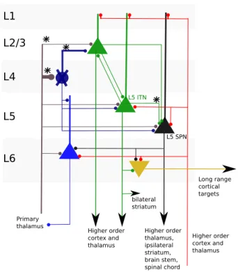
micro-circuit. L1 L2/3 L4 L5 L6 Long range cortical targets Higher order cortex and thalamus bilateral striatum Higher order cortex and thalamus Higher order thalamus, ipsilateral striatum, brain stem, spinal chord Primary thalamus L5 ITN L5 SPN
Figure 1.1: Canonical cortical microcircuit. In this sketch we only show the prin-cipal cells, and we ignore the fact that inside each layer, pyramidal cells tend to connect with cells of the same subclass. This figure was adapted from [59].
There are quantitative differences of this circuit across areas and species [60], but nonetheless, this motif suggests the existence of a basic compu-tational module that is the substrate of the learning and/or the execution
of a full spectrum of high-order functions like fine sensory discrimination, speech, decision making or motor skills. Many people think that the canon-ical microcircuit must play a basic computational role, like the transistor in digital electronics. The transistor is the building block of logical gates (and, or, nand, ...). These logical gates are a very powerful tool, because every Boolean function -correspondence between digital inputs and ouputs-is implementable as a composition of logical gates. In a subsequent chapter we will show an example of a model of a recurrent network that intends to model the fifth layer of the cortex. In this model, when we vary parametri-cally the strength of the connections, we can show theoretiparametri-cally that there is a qualitative difference in way the network operates. Functionally, the first three supragranular layers L1,L2,L3, are the main origin and termination of intra-cortical connections within areas of the same hemisphere or to the opposite hemisphere, through the corpus callosum. The fourth layer (L4) is the main circuit input from the thalamus. In the chapter four, we will expand the discussion about the main thalamocortical projections into the cortex, that synapses mainly onto layer 4 but also in layer 2/3. From layer 4, the information then flows in a feed-forward way to L2/3 and from L2/3 to L5.
Determining the connectivity rules within and across layers is a major challenge that might reveal the computations that are taking place in this circuit. For example Kampa and colleagues [76], recorded simultaneously triplets of neurons, placing one patching electrode in L2/3 and the two others in L5. In a second experiment, they also placed two electrodes in L2/3 and one in L5. By injecting current in one of the three electrodes, it is possible to observe whether they elicit excitatory post-synaptic potentials in the two other electrodes and then obtain a statistical view of the way neurons tend to connect (figure 1.2 left panel). They conclude that pairs of neurons in layer five tend to receive more shared input from cells in L2/3, when they are connected. This suggest that there are sub-networks in layer five that tend to receive specific shared inputs from L2/3 (see figure 1.2), which in turn receive specific inputs from L4, as shown by Callaway’s group in 2005 [164].
In figure 1.1, we marked with an asterisk the main connections that we will consider in this thesis. We will first analyse data from primary so-matosensory and auditory cortex in L5. Layer 5 is a major output projection of the cortex. As we see there are two cell subclasses in layer 5
(intratelen-Stimulate: L5 L2/3
L5 pair connected L5 pair not connected
C
Figure 1.2: Feed forward output of the cortical column. Left panel: experiment to map the connectivity between L2/3 and L5. Right panel: schema the spatial connectivity of the feed forward network going from L4 though L2/3 to L5. Adapted from [76].
cephalic neurons and sub-cerebral projection neurons), which connect asym-metrically, the projections going mainly from intratelencephalic neurons to sub-cerebral projection neurons. However, intratelencephalic neurons tend to have a larger connection probability between themselves with respect to sub-cerebral projection neurons [81]. Also, intratelencephalic neurons tend to show moderate firing rate, whereas sub-cerebral projection neurons have a periodic spatial organisation and can spike in bursts. Finally sub-cerebral projection neurons project to the striatum, the brain stem, and to the spinal chord.
As we mentioned earlier, the whole picture of how the canonical microcir-cuit works is more complex, because we need to add the inter-neurons, which are inhibitory. For example, it has been reported that pyramidal neurons in L6 have a net inhibitory effect on the other cortical layers [110].
1.2
Spontaneous activity in the brain
We refer to spontaneous activity as the brain activity in the absence of an apparent sensory input or motor output. It is also termed resting-state activity, by opposition to evoked activity.
The first reports of spontaneous activity in the brain go back to 1891 when Adolf Beck placed electrodes on the surface of the brain of rabbits and dogs, and observed fluctuating activity. In turn, in 1924, Hans Berger placed electrodes on the scalp of human subjects, and recorded the first human electroencephalogram -EEG-. Using the EEG, Berger reported the existence of alpha waves (7.812 -13.28 Hz) when the subject closed his eyes, and their replacement by faster beta waves (12.5 - 30 Hz), when the subject opened the eyes. Also, he reported alterations in the EEG during epileptic seizures. The EEG was important for the discovery that during sleep, the surface of the brain went through different dynamical regimes, also called cortical states.
With the arrival of multi-unit extracellular recordings in the 2000’s, the neural correlates of the cortical states at the population level started to be explored in animal models.
In addition to the cortex, spontaneous activity has been observed in the retina, in the cochlea, in the spinal cord, in the cerebellum, in the thalamus, in the basal ganglia and in the hyppocampus [16],[61]. Aside from the in-troductory remarks in this chapter, in subsequent chapters we will focus on spontaneous activity in the cortex.
1.2.1
Active and inactive states
Active and inactive states are dynamical properties of a cortical networks, which are known to be recurrently connected. The state qualifies the macro-scopic behaviour of the network, which results from the way neurons fire in relation to each other.
Inactive state designates a regime in which there is strong
synchroni-sation of all the neurons: during the up phases, all neurons fire together, and during the down phases, all neurons are silent, and this is is also vis-ible at the level of the multi-unit activity (MUA), or population firing
rate. This alternation between up and down phases is strictly speaking not
an oscillation, in the sense that the transitions between up and down states are not periodic in time, they seem random, but we will use anyway this terminology in a sloppy way. The slow oscillation has a power spectrum that is concentrated in a frequency band from 0.5 to 4 Hz. Also, because of this sharp transitions between activity and silence, pairs of cells tend to covary together around their respective mean, so that on average, the mean
pairwise correlation - the average of the correlations between all pairs of recorded neurons- is positive (see figure 1.3). Other synonyms of inactive state that are also present in the literature and that we will commonly use are synchronised, inactivated or deactivated.
At the single cell level, the membrane potential makes slow-frequency, large-amplitude changes, that correlate with the up and down phases [30], [131], [142]. The slow oscillation propagates around the different cellular layers of the cortex [131], and across cortical columns and brain areas [61] . The active state (also called activated or desynchronised state), presents on the contrary a more tonic firing rate of the cells, and a constant MUA (see figure 1.3). The histogram of pairwise correlations is centered around zero, with a small but positive mean, so that half of the pairs of cells are positively correlated and half are negatively correlated. At the single cell level, the membrane potential is depolarised close to the firing threshold [166].
In the computational literature that aims at modelling these two brain states there are two technical terms: synchronous, and asynchronous, which have a precise definition, but whose characterisation might be more or less close to the real cortical states.
Both synchronised and desynchronised states states can we identified using the local field potential LFP, which is the extracellular membrane potential generated by the transmembrane currents: in active state the LFP displays little power in the lower frequencies (delta) and high power in the higher frequencies, whereas in inactive state, it follows the alternation be-tween up and down phase, but in an inverted way with respect to the MUA, because the reference is placed extracellularly. Finally, what we call active and inactive state are in reality extremes of a continuum of desynchroni-sation: in certain situations the cortex might be more or less locked to the extremums, and in other situations to have a time varying desynchronisation level.
There is a tight correspondence between the activity in the cortex and the activity in the hippocampus (even if the dynamics in the hippocampus are different). The equivalent of the synchronous state in cortex is called large irregular activity in the hippocampus (LIA), and the equivalent of the desynchronised activity is called hippocampal theta.
0 20 40 60 80 neurons Inactive mua 0 20 40 60 80 neurons Active mua −0.4 −0.2 0 0.2 0.4 corr frequency Correlations Inactive Active
Figure 1.3: Inactive state and active state. The population rasters present 5s of data recorded from layer V in primary auditory cortex. Every dot represents an action potential.
1.3
Brain states and behaviour
1.3.1
Behavioural correlates of spontaneous activity
During sleep, the distinction between cortical states is clear because the difference in the level of desynchronisation between rapid eye movement -REM- and of synchronisation during slow wave sleep -SWS- is very pro-nounced. In SWS the eyes execute rolling movements, whereas in REM sleep the eyes move in random directions.
Both in active as in inactive state, changes in the pupil size correlate very well both with the slow "oscillation" of the synchronous activity also with important changes in the desynchronisation level [98].
In awake state, the cortex wanders between inactive and active state [98]. However, there is still not a complete taxonomy of fine behavioural correlates of both states in awake state.
The effort of relating behaviour with the brain rhythms started in the seventies with the pioneering work of C.H Vanderwolf, that noted the corre-lation of the hippocampal LFP with the ongoing behaviour of the rat [150]: "Trains of rhythmical 6-12 c/sec [hipoccampal theta] waves in the hippocam-pus and medial thalamus precede and accompany gross voluntary types of
(in the alert state) and automatic movement patterns such as blinking, scratching, washing the face, licking or biting the fur, chewing food or lap-ping water are associated with irregular hippocampal activity [LIA]". We now know that theta waves in the hippocampus correlate with desynchroni-sation in the cortex and LIA correlates with synchronidesynchroni-sation.
Futhermore, Poulet and Petersen [119] showed that during these periods of quiet wakefulness, when the cortex was more synchronised, the membrane potential of nearby cells was also highly correlated.
Zagha and colleagues [166] observed recently in 2015 that the mice’s deep layers of motor cortex could stay activated for long periods, even in the case of absence of stimuli or of observable movements. This happened while the animals were achieving good performance in a behavioural paradigm that consisted in withholding from licking and licking after a whisker touch. Interestingly, towards the end of the behavioural session, when the mice were tired and did more mistakes, motor cortex was more desynchronised, in particular before miss trials in comparison to hit trials.
Finer, non subjective quantification of behaviour might help understand-ing the subtleties of the correlation between brain states and awake be-haviour, which will require techniques like video segmentation and machine learning to find regularities between the levels of synchronisation and the behaviour in freely moving conditions. A more controlled approach consists in using head-fixed mice on top of styrofoam balls and closed loop virtual reality environments [62], [107].
1.3.2
Cortical states and attention
Attention refers to the process by which "organisms select a subset of
avail-able information upon which to focus for enhanced processing" [156]. Some examples of attention are: orienting the head towards a strong unexpected sound, focusing on a conversation and do not perceive that someone steals your wallet, or searching for a contact lens on the floor. The first exam-ple is an examexam-ple of bottom-up attention whereas the other two are examples of top-down attention, also called selective attention. The difference between top-down and bottom-up attention depends then on the way of filtering out the information: whether it is provoked by the saliency
of the stimulus characteristics (bottom-up), or whether an instructive signal sharpens our senses to detect and process a particular kind of stimulus at the expense of others. Here we will concentrate in top-down attention effects.
A classic behavioural paradigm to study attention in monkeys was pro-posed by Moran and Desimone in 1985 [103]. A monkey fixates the gaze in a fixation point center, and using its visual periphery it has to solve the task to obtain water. Certain cells in the visual system possess what is called a
receptive field: they spike when a particular type of stimulus is present in
a given region of the visual space. In this experiment, Moran and Desimone recorded cells which spiked when horizontal and vertical red bars -but not green bars-, where presented on their receptive field. In their experiment, both a red bar and a green bar were presented in the receptive field of the recorded cell. By blocks, to solve the trial, the monkey has to pay attention to only one of the two bars, the red or the green bars. To win a drop, the animal has to quickly press a bar when it sees the same orientation in the sample and in the test, otherwise there is no reward. This kind of task is called a match-to-sample task, and by design, the subject needs to pay attention twice in order to be solved. If the response of the recorded cell was purely sensory -and not modulated by attention -, the cell should spike in a similar manner in all conditions. However, what Moran and Desimone found, is that in V4 (fourth cortical visual area) and in IT -inferior temporal
cortex, but not in V1, there are cells which show modulation of attention:
when the effective stimulus (the red bars) was attended either during the sample or during the test, the recorded cell had a strong response, but when the monkey attended the irrelevant stimulus (green bars), the cell was al-most silent, in spite of the presence of the relevant stimulus in the receptive field.
Using a similar behavioural paradigm as Moran [103], Fries and col-leagues showed that attention reduced low frequency synchronisation of V4 neurons that represented the effective stimulus, and importantly, that the observed desynchronisation was local in space. They also showed that at-tention comes with an increase in gamma frequency (35-90 Hz). Finally, Mitchell and colleagues [99], as well as Cohen and Maunsell [26] showed in 2009 that attention reduces variability, noise correlations and low-frequency fluctuations.
Both attention and cortex desynchronisation have many characteristics in common: reduced power in low frequencies of the LFP, reduced trial to
trial variability, and reduced noise correlations [61]. Also, the neuromod-ulatory systems involved in synchronisation, that we will mention in the next section, are also involved in attention. However because the neuro-modulatory systems broadcast signals in a more global way at the level of the cortex, attention involves supplementary mechanisms in order to gain spatial selectivity. Deco and Thiele [34] have proposed, using biophysical simulations, that cholinergic feedback projections from higher cortical areas might mediate local attentional modulation of cortical circuits.
1.4
Neuromodulation
1.4.1
Sleep-wake cycle
The chemical basis of cortical and hippocampal spontaneous activity are studied since the 70’s (see [151]), and in particular the neuromodulators that are responsible for the alternations between sleep and awake and for the variations in brain state in awake and in sleep (REM vs non-REM). The neuromodulators that induce these variations are the noradrenergic system -situated in the locus coeruleus- the glutamatergic system -located in the thalamus- [61], [98] and the cholinergic system, located in the basal forebrain. In the following figure 1.4, we see that during the sleep-wake cycle (cir-cular arrows), J. Allan Hobson [66] shows the covariation of three physiolog-ical variables (activation, modulation and input-output gating). We can see that sleep correlates with low levels of norepinephrine, whereas the levels of acetylcholine might be both high during awake and sleep periods.
Xu and colleagues [163] perturbed optogenetically different cell types in the basal forebrain and were able to elicit wakefulness activating succes-sively cholinergic, glutamatergic and parvalbumin-positive (PV+) GABAer-gic neurons. Reciprocally, they induced non-REM sleep, when activating somatostatin-positive (SOM+) GABAergic neurons.
1.4.2
Effects of acetylcholine and norepinephrine on
the synchronisation level of cortical populations
Goard and Dan [51] showed in 2009, that brief stimulations of the nucleus basalis -a cholinergic nucleus in the basal forebrain- induced strong
decor-High NA and serotonin Waking NREM REM Low A High I Internal External High ACh M a
Figure 1.4: The AIM model of brain-mind state control [66]. A refers to acti-vation, M to modulation and I to input-output gating, the process that controls the access to the sensory information from the external world and which prevents sending motor commands to the muscles.
relation between neurons in the visual cortex of rats. The acetylcholine released by the basal forebrain acts on the interneurons disinhibiting the pyramidal cells in layer 5. Precisely, the fifth layer of the cortex is the place in which the up and down phases are generated to then spread out to the other layers, as shown in slices by Sanchez-Vivez and McCormick [131].
Castro-Alamancos and Gulati [22] showed that the action of the cholin-ergic system and of the noradrencholin-ergic system led to different types of desyn-chronised states: in the case of cholinergic stimulation, the activated state maintained a constant population firing rate with respect to the inacti-vated state, whereas the norepinephrinergic cortical stimulation decreased the overall firing rate.
More recently, in 2013, Polack et al. [118] performed whole cell record-ings in head-fixed mice on a spherical treadmill. By separating the mem-brane potentials of single cells according to whether the mice where running or resting, they computed the distributions of the membrane potentials in both conditions. They found that both during immobility and locomotion, the distribution of membrane potentials was unimodal. However, during lo-comotion the distribution had a larger mean membrane potential, and was sharper, meaning that the variance was smaller. Thereby, they proceed to apply local perfusions of agonists and antagonists of both drugs, and con-cluded that during the resting periods, the cholinergic input was responsible for maintaining unimodal the shape of the distribution of membrane
poten-tials. In turn, norepinephrine was responsible for the depolarisation of the mean membrane potential during locomotion.
In summary, these results show a complex and unfinished picture of what brain states are, and of how they are regulated by the neuromodulatory sys-tems. The picture of an unidimensional continuum between synchronised and desynchronised cortical states may be much less clear and higher di-mensional that we usually think.
1.4.3
Use of anesthesia to study brain states
The use of spherical treadmills and head fixed rodents is very recent. For practical reasons, instead of recording neural activity directly from behaving animals, the traditional approach has been of recording from anaesthetised animals.
The first kind of anaesthetics that where used to study the brain in the 60’s and in the 70’s where barbiturates like the thiopental sodium. However, this drug has a strongly depressing effect and doesn’t induces population dynamics that resemble the ones observed during sleep or awake. In vitro, barbiturates hyperpolarises the membrane potentials, only allowing some rare synaptic events of small amplitude [35]. In vivo, the barbiturates tend to suppress the effects of the recurrent connectivity on the dynamics, letting only the stimulus driven feed-forward component of the currents elicit ac-tivity. This fact was not really understood at the time, but didn’t prevent a whole generation of neuroscientists like Hubel and Wiesel to successfully study sensory processing. When it became evident that ongoing activity was an interesting topic and that it could have an impact on sensory processing, researchers started trying other anaesthetics that don’t preclude it.
Clement et al. [25] showed that it is possible to elicit periods of both high and low synchronisation using urethane anesthesia. In this study they show that state alternation is a cholinergic phenotype and it is independent on norepinephrine. The rate of these brain state alternations did not correlate with variations in the concentration level of urethane. The activity recorded during sleep and after the drugs injection was found to be very similar, both at the level of the physiological correlates (muscular tone, respiration rate, cardiac frequency) as well as in the LFP (Power, time intervals be-tween states). This means that urethane anesthetised animals seems a good preparation to study sleep and brain states.
Pachitariu and colleagues [111] also use alternative anaesthetics: they use ketamine/xylazine to lock the cortex in synchronous state and use fen-tanyl/medetomidine/midazolam to obtain desynchronised states.
1.5
Cortical states and evoked activity
1.5.1
Sensory responses in different cortical states
The study of spontaneous activity is inextricably linked with the study of sensory processing in the brain, because the neural representations result from an interaction of the feed-forward activity coming from the thalamus, with the ongoing activity that is widespread around the cortex. This interac-tion can be quite complex: Curto et al. [31] predict the population responses to clicks on a trial by trial basis, fitting data to a model which is non-linear in the synchronised states and approximately linear in the desynchronized states.
We will examine here the evidence that different cortical states elicit different neural responses in different sensory modalities, the way this im-pacts the fidelity of sensory representations and some of the mechanisms that provoke these differences in the responses across states.
Few years after the first discoveries of Hubel and Wiesel [72],[73], Wurtz replicated their experiments using awake trained monkeys [162]. He con-cluded that the basic organization of the receptive fields in striate cortex was similar to the organisation of the receptive fields in paralysed, anesthetized cats and monkeys measured by Hubel and Wiesel. Surprisingly, Wörgöt-ter et al. [161] found in 1998 that the receptive fields of complex cells are wider in the visual space during synchronized states and smaller during non-synchronized states. Wörgötter reports that, for a 2.5 fold power increase in the range 1-4 Hz, the receptive field grows by 27 %, becoming less selective. Recent findings [12], [107] point at increases in neural responsiveness as the cortex desynchronises during locomotion. In these studies, drifting grat-ings are presented to head fixed mice while the mice lay on a treadmill, and cells are recorded in the primary visual area (V1). These studies consistently
report additive and multiplicative gains of the tuning curves in V1 during
desynchronised state. The anatomical projection from motor cortex to au-ditory cortex that might be involved in these locomotion-associated changes of auditory cortical response was described by Schneider et al. [133].
Marguet and Harris [96] presented amplitude modulated noise stimuli to urethane anesthetised rats, and asked to which extent they could pre-dict single neural activities based on the LFP or on the stimulus. During desynchronised activity, the neural activity could be predicted from both the stimulus and the LFP. For the synchronised activity, they found that the activity of individual neurons was strongly predictable from the LFP and poorly predictable from the AM noise envelope. Therefore, in presence of such AM noisy stimuli, the cortical activity is largely decoupled from the stimulus. This doesn’t mean that during synchronised activity, the cortex can not be entrained by external stimuli: for more punctuate stimuli like clicks or tones, the cortex responds reliably transitioning from a down phase to an up phase [89], [31].
In auditory cortex of gerbils, Pachitaru and colleagues [111] probed the population response with other stimuli. Using pure tones, frequency modu-lated tones and speech, they concluded that the responsiveness, the selectiv-ity, the reliability and the temporal precision of the population was higher during desynchronised state than during the synchronised state. Another relevant aspect of this study is that it examines how the representation ca-pacity of auditory cortex is modified as a function of the states, i.e. to which extent different sounds evoke different population responses. The authors found that when presenting different speech sounds, the similarity between the responses was higher during the synchronised states than during the desynchronised state.
A PSTH or the peri-stimulus time histogram is the average response of a cell following the presentation of a stimulus. When plotting the PSTH of auditory cells at their best response frequency, Pachitaru and colleagues, find that if the brain could average out the slow oscillation in a single trial, it would find on average similar responses -not perfectly although- in both active and inactive states. However these responses are more variable in inactive states [12], [99].
Given the evidence from the literature, it seems that the information quality about the details of a stimulus conveyed by the neural populations is smaller in the inactive state with respect to the active state. Is the syn-chronised state during awake a watchful state of lower energy consumption, whose first role is not to encode properly all the details of a stimulus, but to facilitate the detection of stimulus onsets, so that the cortex desynchronises in case of danger for example?
Fanselow and Nicolelis do conclude in this direction in a study in so-matosensory cortex [40]: "in the absence of whisker movements (quiet im-mobility), somatosensory neurons seem to be highly responsive to punctuate tactile stimuli but not to sequences of stimuli. In contrast, during the whisk-ing state, when active exploratory whisker movements are used by the rat to gather tactile information, the temporal fidelity of sensory responses to rapidly presented stimuli is enhanced".
This difference in population response depending on the frequency of the stimuli is explained by Castro Alamancos [23] by the finding that the rapid
sensory adaptation depends on the cortical state. Rapid adaptation is the
decrease in the response of a neuron to a high frequency stimulus. We call it rapid, because it acts on a time scale of 100 ms. Castro Alamancos finds that during the desynchronised state, there is little adaptation whereas during synchronised state there is strong adaptation. The mechanisms advanced for the cortical adaptation are the depression of the thalamo-cortical synapses and an increase in inhibition.
As advanced by Castro Alamancos [23], the system might adapt its brain state and its response to stimuli to meet information processing demands dictated by behavioural contingencies. Luczak [89] recalls that the appar-ently noisy slow oscillation that might seem to degrade perception might in fact be the result of hidden variables that aren’t under experimental con-trol : "Only a small fraction of the input to a cortical column arises from primary sensory thalamus, and responses in sensory cortex can be affected by cognitive factors such as reward and attention, other sensory modalities, and ongoing oscillations".
1.5.2
How could the brain distinguish spontaneous
ac-tivity from evoked acac-tivity ?
As we saw in previous sections, it seems that the brain state impacts the sensory representations in a way that seems to be adapted both to the en-vironment and to what the animal is doing. It is possible that this mode of operation be a way of reconciling rest and alertness, allocating the attention according to the behavioural needs [61].
During desynchronised state, the stimulus evoked dynamics dominate the activity [96], and the representation capacity of the cortex is higher than during synchronised activity [111]. During synchronised state, the extended
stimuli are filtered out, and the slow oscillation dominates the dynamics, over the evoked activity [96]. However, punctual stimuli provoke down to up phase transitions and behavioural responses[30], [157]. One of the questions that arises if we suppose that the sensory processing pipeline is serial -is: how can the upstream cortical circuits distinguish between an up-phase transition elicited by a sensory stimulus, from an internally generated one ? And more generally, in both states, how is the brain able distinguish between the evoked and the spontaneous activity [157], knowing that the range of firing during the spontaneous activity is of the same magnitude as the range of evoked activity? We consider several hypothesis.
1.5.2.1 Noise subtraction hypothesis
One first hypothesis is that the brain subtracts out some kind of efferent copy, so we can’t hear our own noise, as that it happens with tickling (we can’t tickle ourselves). This hypothesis would fit well with some signal like the synchronous state, that spreads around all the cortex: it suffices that some downstream area process the difference between the feed-forward input from a lower area and from some neighbour cortical area that is not concerned with audition, but who is affected by the synchronous activity.
1.5.2.2 Different time scales over the cortical hierarchy filter out
the non-perceptually related activity patterns
One important feature of the brain is that the information processing units, the neurons, receive currents, and emit spikes on a time scale of the order of milliseconds, whereas the time scales at which the behaviours happens is at least of the order of tenths of a second. One possibility to reconciliate this apparent over-sampling of the world with the time scale on which the body acts on the world, is that somehow in order to form percepts, the incoming information is accumulated at different stages of the perceptual pyramid, and each intermediary unit of perception is only active when many of the units that project to it are active. In that way, as we go up the processing hierarchy, the time scale of the units increases also.
If we consider that the spontaneous activity as a sequence of incoherent neural patterns, we can think that only the stimuli, simply due to their tem-poral persistence in the environment, are going to repeatedly elicit sequences of identical patterns which are going to elicit higher order representations.
The randomly generated sequences of neural patterns, because of their tem-poral incoherence, are not going to pass through the different processing stages.
Murray et al. [106] show experimentally the existence of a hierarchical ordering in the time scale of in the intrinsic fluctuations in spiking activity of spike trains recorded in monkeys engaged in cognitive tasks. The authors simply measured the width of the spike trains autocorrelation in different brain areas: in more sensory areas they found shorter time scales, whereas in pre-frontal areas, they found longer time-scales.
In their interpretation of this observation, the role of the time scales on the cortical hierarchy is similar to the one advanced here, even if they doesn’t comment on the spontaneous activity: "shorter time-scales in sen-sory areas enable them to rapidly detect or faithfully track dynamic stimuli. By contrast, pre-frontal areas can utilize longer time-scales to integrate in-formation and improve the signal-to-noise ratio in short-term memory or decision-making computations".
1.5.2.3 Signal and noise have different directions in neural space
Another possibility, is that the spontaneous and the evoked activities live in orthogonal subspaces. In their seminal paper, Kaufman and colleagues [78] proposed a simple but very elegant mechanism by which determined areas could isolate themselves from surrounding areas to do some local processing, despite the fact that they are physically connected to these areas and also communicate with them. During a reaching task, a monkey has to see a light on a screen and withhold from reaching it before a go cue appears. When the go cue is on, the monkey must touch the place where the light was, in order to receive a reward. Parallel recordings show that the premotor cortex is very active during the hold period. The question is: why this pre-motor activity doesn’t trigger movement despite the fact that it projects to the motor cortex, whose activity correlates with the muscle activity ? They propose that as long as the activity in the pre-motor cortex lives in a null space, motor cortex doesn’t see the difference. Lets take for example two neurons in pre-motor cortex which project to a neuron in motor cortex. The activity of this neuron innervates a muscle, with a strength proportional to its firing. As long as the sum of the activities of the pre-synaptic neurons is constant: p1+p2 = (p1+κ)+(p2−κ) = C, the post-synaptic currents in motor
cortex are constant also. When the activity of both neurons increase, the direction that causes more effect on the post-synaptic current is the direction orthogonal to the null space, called the output potent space: (p1+ κ) + (p2+
κ) = C + 2κ. Then, we can have local processing - preparatory
activity-happening in pre-motor that motor cortex doesn’t see, and communication between the areas after the go cue.
Similarly it could be that the spontaneous activity lives on a subspace on a low area of the cortical hierarchy, but when a stimulus arrives, the circuit responds in such a way that the elicited activity has a certain direction that excites the next processing stage of the perceptual chain. Then, different processing areas might be isolated, and the spontaneous activity might serve as substrate for computations.
1.6
Possible roles of spontaneous activity
Even though there were early reports in the 1970’s pointing at correlations between behaviour and the ongoing activity [79],[150] this activity was con-sidered until the 90’s like a noise [145], a fundamental limitation or a by-product of the system, which constrained the discrimination of sensory re-sponses [157]. Some authors have argued against this noise hypothesis due to the important metabolic cost of spiking [5], suggesting that spontaneous activity might actually play a functional role in the brain. In what follows, we will review some of the advanced hypothesis.
1.6.1
Developmental role
Increasing evidence points at the fact that spontaneous activity might play a fundamental role in the development of neurons and in their connections. In the mainstream theory of brain development, genetic programs orga-nize the main projections, for example from the retina to the brain. Later, the visual experience leads to a refinement of the connections. However, more and more observations reveal that in fact genetic programs and neural activity interact at all phases of development and determine the composition and the organisation of neural circuits [16]. In early phases, when neurons are still not connected, spontaneous activity affects neuronal differentiation, establishment of neurotransmitter phenotype, and neuronal migration [140].
Later, spontaneous activity seem to have the role of providing an instruc-tive signal for the establishement of the functional connections, for example in motor neuron path finding [58], or in the formation of sensory maps [77]. However as Blankenship and Feller point out [16], disambiguating the causality between the activity and development is not easy: "Insights into how spontaneous correlated activity influences the development of neural circuits will require manipulations that alter the pattern of activity rather than block it entirely".
1.6.2
Memory consolidation
Following severe seizures that had no treatment at the time, the patient H.M. went though a bilateral medial temporal lobe resection. Following the surgical operation, Scolville and Milner [135], performed several neuro-psychological tests on H.M. and concluded that the hyppocampus had a decisive role in the formation of new memories and in the retrieval of recent memories, but not in the retrieval of oldest memories, which remained intact. Influenced by these pioneering results, and by David Marr’s [97] theory about memory, the actual theory about the role of the hyppocampus is named the "two stage theory of memory". This hypothesis postulates that the memories are initially created and stored in the hippocampus. During sleep, these memories would be reactivated and transferred to the medial pre-frontal cortex mPFC, where they would be stored more permanently in a process called consolidation, that involves reorganization and strengthening of the cortical memory trace. In parallel, as the mPFC becomes more involved in recalling the memories, the hippocampus disengages progressively.
Experimental studies have brought evidence of an interaction between the hippocampus and the cortex that involves different types of waves. The first studies showed correlational evidence of a coupling between the tran-sitions to the up phase of synchronous activity -that happen in cortex- and sharp wave bursts in the hippocampus [10],[138]. Bennett and colleagues [12] advanced the hypothesis that the condensed joint spiking in the up phases of the synchronous state might have a role magnifying post-synaptic responses and facilitating spike-timing dependent plasticity -STDP.
Very recently, the role of the coupling between hippocampus and cortex in memory consolidation was demonstrated causally [95]. Rats were first placed on an arena in which there were two objects. When sharp wave ripples
were detected in the hippocampus, the mPFC was stimulated electrically in closed loop. Finally, the rats were put back in the arena containing the objects, having previously displaced one of the two objects. To have a behavioural readout of the memory, they quantified the time that the rats spent close to the displaced object, which was interpreted as a readout of memory or novelty.
Indeed, it was the case that rats spent more time close to the displaced object when the stimulation protocol was precisely time locked, and not when the stimulation was applied with a random delay after the detection.
1.6.3
Bayesian inference
One very innovative hypothesis about what perception is and how it occurs, is that perception can be understood as a Bayesian inference process, i.e. a process that aims at deducing which objects we are experiencing in the external world, given noisy evidence and prior information about the context. As pointed out by Kok and de Lange [44], the motivation for developing such kind of models is that "perception is not solely determined by the input to our eyes, but it is strongly influenced by our expectations".
Lets imagine for example that x is a scalar variable that quantifies an unidimensional stimulus, for example a sound pressure wave of the voice of a person. x might come from two persons called 1 and 2, whose respective voices y1 or y2 may have different distribution of frequencies. Given that
the environment is noisy, the perception that will try to infer is the joint distribution of the possible causes of x, p(Y1, Y2|x), through Bayes rule, and
ultimately y1 or y2, so that we know who is talking.
p(Y1, Y2|X) =
p(X|Y1, Y2)p(Y1, Y2)
Z
p(Y1, Y2) is the prior distribution of inputs, it describes the learnt
reg-ularities about the sensory environment, in this example the joint power spectrum of the two persons. p(X|Y1, Y2) is called the likelihood, it assumes
that we have a model of the environment that allow us to evaluate how likely would the observation x be, if we knew the values of the two features y1 and
y2. Z = p(X) is a constant with respect to Y1 and Y2. Finally p(Y1, Y2|X) is
the posterior distribution, from which we deduce p(Y1 = y1, Y2 = y2|X = x).
(from the regions where the prior p(Y1, Y2) is not nil), and the model of
the world that we have, given the sensory evidence. If the prior is flat for example, the posterior will reflect simply our model of the world.
Lets imagine that the receptive field of one toy neuron is a frequency band of low pitch with a mean of 100 Hz, and a variance of 20 Hz. In time, the firing rate of this toy neuron fires at a mean of 100 Hz, and has a variance of 20 Hz: the instantaneous firing rate represents the probability of taking a certain value, as if this neuron was sampling from the distribution of fre-quency corresponding to the receptive field. Under this "sampling-based" hypothesis, if in the brain neural populations somehow use this represen-tation, this framework [42] proposes an interpretation of what spontaneous activity might be: in the absence of sensory stimulation x, the posterior dis-tribution is similar to the prior disdis-tribution, and the spontaneous activity reflects this prior. One of the predictions of this framework is that spon-taneous activity is similar to the evoked activity, which has been observed many times [80], [43], [89] (we will comment more on this point). Another possible consequence is that on the motor side this spontaneous activity could have a role in preparing actions, so that animals are ready to respond faster. Overall, this bayesian sampling theory shows normatively how to combine the priors, the top-down expectations about the world with the sensory evidence about it, and precisely the spontaneous activity plays the role of reflecting those priors about the world.
A more mathematically involved theory called predictive coding [44], also based on Bayesian inference, conjectures that each region of the cortical hierarchy makes hypothesis about its incoming inputs. In this theory, each region generates a hypothesis about the incoming input, and feeds the error (the difference between the model and the input), to the upstream region, and feed-backs the more consistent hypothesis, to the downstream region. After several iterations, the predicted error is small in all regions and an hypothesis about the source that generated the sensory stimulus is retained. A whole literature testing some of the ideas of predictive coding exists. Let’s only cite Sadaghiani and colleagues [130] which performed a detection task with humans on a magnetic resonance imager. The authors observed that consistently, in the trials in which the subjects reported having heard a dim sound, the spontaneous activity in auditory cortex that preceded the presentation of the sound was significantly higher in hit trials with respect to miss trials.