Praia de Botafogo, nO 190/10° andar - Rio de Janeiro - 22253-900
Seminários de Pesquisa Econômica I (2
a
parte)
IITREND, UNIT ROOT AND
STRUCTURAL CHANGE IN
MACROECONOMIC TIME SERIES
11
Pierre Perron
\marf.
(Universidade de Montreal)
Coordenação: Prof. Pedro Cavalcanti Ferreira Tel: 536-9353
112 Unit Roots and Cointegration
Johansen ML Procedure (trended case, trend in DGP)
Coin'egration LR 'ut Itatistics Samp/e period: 1967: 2 to 1991 : 2 p
=
2 1(1) variables included: C, I. 1(0) variables included: W DD682, DD792, DD883. Null r=O r51 Null r=O r 51 Table 3A.6Tests for Cointegration: 2 Variable VAR
Alternative r
=
1 r=2 Table 3A.7 Statistic 21.58 0.344,Testa for Cointegration: 2 Variable VAR
Alternative r ~ 1 r=2 Statis'ic 21.93 0.344 95%CV 14.07 3.76 95%CV 15.41 3.76
We cooclude with a oote of cautioo. A time series plot of the residuais of the cointegrating vedor, adjusted for short ruo dynamics (see the Microlit maoual for details) suggests some substaotial departure from stationarity io the latter part of the estimatioo period. This is the case irrespective of which coin-tegratiog vector we choose to believe. Whilst formal tests cao-not reject coiotegration, inspection of residual plots casts serious doubt 00 their validity. .
00
ccrW/f"7~C4' ~
}?R
Atr~
&-c- ____
sb
(" 15
($.-
;?~o"
.
.iZo-t " )
0"áC
;:y/~~~f').
,_"1
4
Trend, U nit Root and
Structural Change in
Macroeconomic Time Series
Pierre Perron·
4.1 INTRODUCTION
The uoit root hypothesis has attraded a coosiderable amount of work in both the ecooomics aod statistics literature. Iodeed, the view that most ecooomic time series are characterized by a stocbastic rather thao deterministic noostatiooarity has become prevalent. The semioal study of Nelson aod Plosser (1982) which fouod that most macroecooomic variables have a univariate time series structure with a unit root has catalysed a burgeoning re-search program with both empirical aod theoretical dimeosions.
As far as macroecooomic theories are coocerned, the most important implication of the unit root revolutioo, is that uo-der this hypothesis random shocks have a permaneot efred 00
the system. Fluctuatioos are oot transitory. This implication, as forcefully argued by Nelsoo aod Plosser, has profouod coo-sequences for busioess cycle theories. It ruos couoter to the prevailing view that busioess cycles are transitory fluduatioos around a more or less stable treod path. It is therefore impor-tant to assess carefully the reliability of the unit root hypothesis as an empirical facto
We have recently suggested that the widespread evidence of unit roots in the univariate represeotation of time series may be due to the preseoce of important strudural changes io their trend fundionj see Perroo (1989). lo that paper, we developed procedures that test for a unit root allowing the possibility of a
• Financiai 8upport in acknowledged from the National Science Foun-dation, the Fonds pour la Formation de Chercheurs de l'Aide à la Recherche du Québec and the Université de Montréal (C.A.F.I.R.).
, 114 Unít Root and Structural Change
one-time struetural change in the trend funetion. The changes considered were of three kinds: a change in intercept (e.g. a crash), a change in slope (e.g. a produetivity slow-down) or both. This simple case of a one-time change may appear overly restrictive. However, its motivation stems from its apparent rel-evance to many historical time series. Indeed, empirical appli-cations using these tests on the same series analyzed by Nelson and Plosser gave evidence that weakens considerably the case for the unit root hypothesis.
The approach is in the spirit of the 'intervention analysis' of Box and Tiao (1975). According to their methodology, 'aberrant' or 'outlying' events can be separated from the noise function and be modeUed as changes or 'interventions' in the deterministic part of lhe general time series model. Using such a strategy makes it "possible to distinguish between what can and what cannot be explained by the noise"j Box and Tiao (1975), p.72. These 'interventions' are assumed to be exogenous and to occur at a known ,date.
We certainly do not entertain the view that the trend func-tion induding its changes are deterministic. This would imply that one would be able to forecast with certainty future changes. This is indeed quite unappealing. What we have in mind in spec-ifying our class of maintained hypotheses is a more general model where the intercept and the slope of the trend funetions are themselves random variables modelled as integrated processes. However, the important distinetion would be that the timing of the occurrence of the shocks affeeting these parameters are rare relative to the sequence of innovations driving the stationary or cyclical component. The intuitive idea behind this type of mod-eling is that the coefficients of the trend funetion are determined by Iong-term economic fundamentaIs (e.g. the strueture of the economic organization, population growth, etc.) and that these fundamentais are rarely changed. In this sense, the exogeneity assumption about the changes in the trend funetion is a device that allows to take these shocks ou t of the noise funetion into the trend funetion without specific modeling of the stochastic behaviour of the intercept and the slope.
This postulate concerning the exogeneity of the break date has been criticized most notably by Christiano (1988) who ar-gued that the choice of these dates had to be viewed, to large
Perron 115
extent, as being correlated with the data. This is an important problem because both the finite sample and asymptotic distribu-tions of the statistics depend upon the extent of the correlation between the choice of the break points and the data. There is a sense in which the choice of these dates can be regarded as independent of the data. First, the dates reported in Perron (1989), 1929 for the Great Crash and 1973 for the start of the produetivity slow-down, were chosen ex-ante and not modified ex-posto Secondly, these dates are related to exogenous events that then occurred and for which economic theory would suggest the effects that aetuaUy happened; e.g. the stock market crash of 1929 with the ensuing dismantle of the economic organization and the exogenous sudden change in oH prices with the resulting alteration of international economic coordination and policies.
In the sense described above the choice of the dates can be viewed as uncorrelated with the data. There is, however, a valid-ity to the argument that it is only ex-post (after looking at the data) that we can say that the changes that followed these exoge-nous events aetually occurred as predieted by the theory. Fur-thermore, many other exogenous events did not have the major impaet that some theories would have likely predieted. In this sense, the choice of the break points must be viewed as being correlated, at least to some extent, with the data. To what ex-tent were the choices of 1929 and 1973 correlated with the data? This is a difficult and praetically impossible question to answer. At the very least, however, these choices were not perfectly cor-related with the data as Perron (1989) did not systematically try various dates to maximize the chances that the unit root would be rejeeted; nor was there any systematic attempt to find where, according to some test cri teria, are the most likely dates of change.
While the assumption about the exogeneity of the choice of the break point is probably a good first approximation to the true extent of the correlation with the data, it is useful to inves-tigate how robust the results are to different postulates. Recent papers have addressed such issues and derived test procedures that explicitly incorporate methods to endogeneize the break date in such a way that it is fully determined by the data. This extreme case is instruetive to study because ir the unit root can still be rejeeted under such a scenario it must be the case that
'r .,.
"l
t
116 Unit Root and Structural Change"
it would be rejected under less stringent assumptions. Papers that have addressed such issues are those of Banerjee, Lums-daine and Stock (1992), Perron (1990b), Perron and Vogelsang (1992, 1993) and Zivot and Andrews (1992).
The aim of this paper is to review the main arguments pre-sented in Perron (1989) and the test procedures subsequently developed with a focus on providing a comprehensive treatment useful to applied researchers. Along the way, we shall illustrate the relevance of these methods using an historical data set of real GDP series for eleven countriesj viz. Australia, Canada, Denmark, Finland, France, Germany, Italy, Norway, Sweden, the United Kingdom and the United States. The data span the period 1870-1986 (except for Finland for which it span 1900-1986) and are the same series used by Kormendi and Meguire (1990)1. Empirical studies using similar sedes deflated by a population index (i.e. real per capita GDP series) include Ben-David and Papell (1992), Perron (1992) and Raj (1992). We focus bere 00 real GDP series instead of their per capita counter-parts since tbey allow us to illustrate the usefulness of a wider range of models.
The outline of tbe paper is as follows. Section 4.2 presents the statistical models used to analyze the unit root issue allowing for a one- time change in tbe slope of the trend function. Section 4.3 discusses the empirical relevance of tbese models in relation to the data set introduced above. Section 4.4 presents simulation results showing that standard unit root tests are biased towards non-rejection of the unit root bypothesis if the data are charac-terized by stationary fluctuations around a trend function that exhibits a structural change. Section 4.5 discusses the statistical procedures tbat allow formal tests of the unit root hypothesis.
1. The data set analyzed here was obtained tbrougb the editorial office of tbe Journal of Money, Cretlil anti Banking. The series are annual real
GDP except for the United States for which real GNP is used from the Na-tional Income and Products Accounts for the period 1929-1986, spliced to Romer's (1989) estimates for the period 1871l-1928. For the United King-dom the series are from Feinstein (1972) for the period 1871l-1947 spliced to the International Financiai Statistics (IFS) series of the International Monetary Fund for the period 1948-1986. For the remaining countries, the series are from Maddison (1982) apliced to the post-war IFS data. Ali series are analyzed uaing a logarithmic tranaformation.
Perron 117
We discuss, in particular, how the asymptotic criticai values de-pend on the specific model analyzed and the method used to select the break date. Tables of criticai values are provided. Section 4.6 presents empirical applications of these methods us-ing the multi-country historical data set. Section 4.7 offers some concluding comments.
4.2 THE MODELS
The null bypothesis considered is that a given series {II.}I (of which a sample of size T+ 1 ia available) ia a realization of a time series process characterized by the presence of a unit root and a possibly non-zero drift. However, the approach is generalized to allow a one-time change in the strueture oceurring at a time T, (1 < T. < T). Three different mo deis are considered under the nuU hypothesis: one that permits an exogenous change in the levei of the series (a 'erash'), one that permits an exogenous change in the rate or growth and one that allows both changes.
As discussed in the introduction, one can view the structural changes to the trend function as some kind or "big shocks" or infrequent events that have permanent effects on the leveI or the series. It is important to take into consideration the way these "big shocks" affect the levei or the variables, i.e. the way the transition to a new trend path oeeurs. In Perron (1989), two models were introduced that have different implications with re-spect to this transition effect. Following the terminology in Box and Tiao (1975» the first islabelled the "additive outlier model" and specifies that the ehange to the new trend function occurs instantaneously. The second is labelled the "innovational outlier model" and specifies that the change to the new trend runction is gradual. Of course, there is an infinity or ways that are possible, in principie, to model gradual changes rollowing the occurrence or a "big shock". One way out or this difficulty is to suppose that the variables respond to the "big shocks" the same way as they respond to the so-called "regular shocks" (the shocks associated with the stationary noise component or the series). Tbis is the approach taken in the modelization of the "innovational outlier model" following tbe treatment of intervention analyses in Box and Tiao (1975).
The distinction between the additive and innovatiooal outlier models is important not only because the assumed transition
O'
i'-I
'i '
~~ ~.
118 Uoit Root and Structural Change
paths are different but also because the statistical procedures to test for unit roots are also different as we shaU see in Section 4.5.
4.2.1 The Additive OutUer Modela
The additive outlier models are specified as follows for each of the three specifications for the types of changes occurring at the break date whicb we denote by T. :
Model (1) !I,
=
PI+
fJt+
(p, - Pl)DU,+
li, (1)Model (2) li,
=
Pl+
fJlt+
(p, - p.)DU,+
(fJ, - fJdDT"+
li, (2)Model (3) li'
=
P+
fJl t+
(fJ, - fJ')DTi+
li, (3)where DU,
=
1, DTi=
t - T. if t>
T. and O otherwise. The noise component li, is of the (orm A(L)II,=
B(L)e" e, ,.. IID.(O,er'), with A(L) and B(L) pth and qth order polynomials,
re-spectively, in the lag operator L. The innovation series {1I1} is taken to be o()f the ARM A(p, q) type with the orders p and q pos-sibly unknown. This postulate allows the series {v,} to represent quite general processes. The nuU hypothesis specifies that a root of the autoregressive polynomial is one, i.e. that we can write
A(L)
=
(1-L)A. (L) where alI the roots of A. (L) are outside the unit circle. Under the alternative hypothesis of stationary fluctu-ations around the trend function all the roots of A(L) are strictly outside the unit circle. Note that the changes in the trend func-tion are allowed to occur under both the null and alternative hypotneses.Model (1) describes what we shalI refer to as the eras h modei. lt allows for a one-time change in the intercept of the trend function. Model (2) alIows both a change in the intercept and the slope of the trend function to take place simultaneously, i.e. a sudden change in levei followed by a different growth path. As in Model (1), the segments of the trend function are, in general, not joined at the time of break. Model (3) is referred to as the "changing growth" model. lt allows for a change in the slope of the trend function without any sudden change in the levei at the time of the break. This implies that the two segments of the trend fundion are joined at the time of break.
119 Perroo
4.2.2 The Innovational Outlier Modela
The innovational outlier mo deis are easier to characterize by de-scribing them separately under the nuU and alternative hypothe-ses. Note also that the innovational outlier versions have been considered only for Models (1) and (2). The basic reason is that the innovational outlier version of Model (3) does not lend itself easily to empirical applications using linear estimation methods. We recall from the above discussion that the innovational outlier model specifies that the "shocks" (or changes) to the trend function affect the levei of the series the same way as the "regular shocks" do. The temporal effect of random shocks is easily analyzed using the moving average representation of the stochastic component. Under the nuU hypothesis, this leads us to the following repreaentations:
Model (1) li'
=
111-1+
b+
1/I(L)(el+
6D(T.)I).Model (2) 111
=
111-1+
b+
1/I(L)(e,+
6D(T.),+
"DU.).where D(T.),
=
1 if t=
T. + 1 and O otherwise. Here, the moving average representation of the first-differences of the data is spec-ified by the lag polynomial1/l(L) (possibly infinite with 1/1(0)=
1). That is, denoting by %, the noise function of the series, we haveAl(L)z.
=
Bl(L)e, and 1/I(L)=
Al(L)-1 Bl(L). Throughout, it is as-sumed that the finite order polynomials Al(L) and Bl(L) have all their roots outside the unit circle. Under this specification we have, for Model (1), that the immediate impact of the change in the intercept is 6 while the long run impact is 1/1(1)6. Similarly, under Model (2), the immediate impact of the change in slope is " while the long run impad is 1/1(1)".Under the alternative hypothesis of stationary fluctuations, the models are:
Model(1)
III=P+fJt+~(L)(el+8DUI)
(4)Model (2) 111
=
IA+
fJt+
~(L)(el
+
8DU.+
-yDT;) (5) where~(L)
= (1-oL)-1 Al(L)-1 BI(L) with A1(L) and BI(L) as de-fined before. In Models (1) and (2), the immediate impact ofthe change in the intercept of the trend fundion ia 8 while the long run impact is
~(1)8.
Similarly, in Model (2), the immediate impact of the change in slope is -y while the long run impad is ~(lh·~! , ~ ,ji ir~ if~·
120 Uoit Root aod Structural Cbaoge
The models under the null and alternative hypotheses can be nested in the following way. For Model (1), we have:
""
y,
=
JJ+
9DU, + fJt+
6D(TB), + 011'-1+
E
CjÔY,_i+
e,
(6) 1=1and for Model (2)
""
1/,
=
JJ+
9DU, + fJt+
'1DT; + 6D(TB), + 011'-1+
E
CjÔY,_1+
e,.
(7) 1=1The coefficient Cj in (6) and (7) correspond to the autoregressive
representation of the moving-average polynomial AI(L)-IBt(L) given by q,(L)
=
(cIL+
c,L2+ ... )
=
tP(L)-1=
BI(L)-I At(L). Thepolynomial q,(L) will be of infinite order if moving average com-ponents are present, i.e. if BI(L) ~ 1. In practice, this infinite sum will, of course, be approximated by a finite sum in order to derive operational tests.
The null hypothesis imposes the following restrictions on the coefficients. For model (6), these are o
=
1,9=
fJ=
O and, in general, 61:0 (if there is a change in the intercept). For Model (7), the restrictions are o=
1, fJ=
'1=
O and again, in general,6 ~ O. Under the alternative hypothesis, we have the foUowing specifications:
101
< 1 and, in general,6
=
O
in both Models (6) and (7). These restrictions are, however, not imposed by the testing procedures described latter.4.3 MOTIVATION
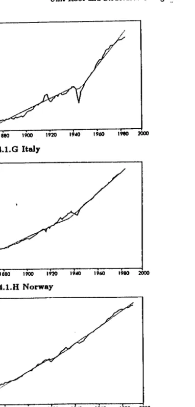
To motivate the models presented in Section 4.2, we consider the historical data set of real GDP series described in the intro-duction. Figure 4.1 presents the graph of each series. A marked characteristic is first the noticeable pattern of increase through time. Hence, the series can be said to be trending. However, this increase over time does not, for most countries, follow a steady pattern. Instead, many series are seen to exhibit one or more of the following features: (i) a more or less sudden decrease in levei (e.g. after the first World War for the U.K., during the Great Depression for Canada and the United States, during World War 11 for France, Germany, Italy and Norway)j (ii) a change in the rate of growth (e.g. after 1940 for Australia, after the Great De-pression for Canada, after World War 11 for France, Germany, Italy and Norway). A feature of interest is that major changes in
Perroo 121
leveis andfor slopes seem to occur only once in the sample con-sidered. In particular when changes in both the levei and slope occur, they seem to do so roughly at the same time (e.g. France, Germany and Italy). This is not to say that other changes in levei andfor slope do not occur for some series but rather that if they do their magnitude are smaU compared to the changes de-scribed previously. This observation supports our claim that the restricted case for which the trend function changes only once appears to be of substantial relevance in practice.
A second feature of interest is that the transition path to a new trend appears to occur gradually, especially when a change in leveI is involved. This suggests that when using Models (1) and (2), the innovational outlier version would be more appro-priate. After visual inspection of the data, it was decided to apply the following models to each country: Innovational Out-Uer Model (1) for the United Kingdom and the United Statesj Innovational Outlier Model (2) for Canada, Denmark, Finland, France, Germany, Italy and Swedenj and Additive Outlier Model (3) for Australia and Norway.
Some comments are in order to offer guidance as to the ap-propriate choice of models in general. Note first that Model (2) is the most general and allow, as possible subsets, changes de-scribed in Models (1) and (3). Model (2) could therefore be used for all series. The problem with this approach is that it may lead to tests with lower power compared to what could be obtained using a more constrained model. As will be seen in Section 4.5, the asymptotic criticai values are the highest under Model (2). There is therefore an advantage to select a model contain-ing no irrelevant regressors, for example in selectcontain-ing Model (1) over Model (2) if no change in slope is apparent and, similarly, Model (3) over Model (2) when a change in slope is apparent but not a change in leveI. However, care must be exercised not to select a model that is too constrained since this would imply a substantial loss in power and even tests that are potentially inconsistent. When in doubt, one should start with Model (2) since it is more general. However, a good practical rule is to
as-sess the robustness of non-rejections of the unit root to different model selections.
The dotted line in each graph represents the fitted trend function. Each non-linear trend function is obtained using the
122 Unit Root and Structural Change Perron 123 5.5. ~5. ~ I A.5 J. 2. 3.S I. '2 . .;J, • •
.
1;~ 1900 .910 1920 1930 1950 1960 1970 1980 1990Figure 4.1.A Australla Figure 4.1.D Finland
8.5
,J
7.51ri
/
l. 7 6. 2 6 1 1860 1880 1900 1920 19AO 1960 1980 2ÓOO 5.~-.---uiso 1920 1860 1900 19AO 1960 .980 2000Figure 4.1.B Canada Figure 4.1.E France
6.5 6 7 J /~ S.S 7 5 6.5 A.5 6 5.5 J.5 ~ J I 'l' A.S 2.
1860 li80 1900 1920 19AO 1960 1980 :zooo
A.
1860 1880 .900 1920 19AO 1960 .980 2000
• Figure 4.1. C Denmark Figure 4.1.F Germany
l
~!i~ ~
1
,1 ~. !.f.,.
f~· ,,'~ . .,
(124 Unit Root and Strudural Change
13.5 13 12.5 12 11.5 11 105 10 i 11180 1900 1920 19~ 1960 1980 2000 1860 Figure 4.1.G Italy 6 5.5 ~.5 3.5 2.5 21 i i i
,
i iI
1860 1880 1900 1920 19~ 1960 1980 2000 Figure 4.1.H Norway 6.56~
/
5.5 ~.5 3.5 2.5 • lIi80 1900 1920 19~0 1980 1860 1960 2000 Figure 4.1.1 Sweden Perron 125 61 1 55 ~5 3.5~ ,.ç.' l i i.
1860 1880 1900 1920 19~0 1960 1980 2000Figure 4.1.J United Kingdom 11 10.5 10 9.5 9 8.5 8 7.5 7 651 i 1860 1880 1900 1920 19AO 1960 1980 2000
Figure 4.1.K United Statea
appropriate model under the aIternative hypothesis. As stated, only one break date was allowed and is as stated in each graph for the
di(feren~
countries. We postpone until Section 4.6, the precise method under which these break dates were seIected. For Australia and Norway the trend functions show a kink at the time of the break since the model selected for these countries is the additive outlier version of Model (3). In these cases, the trend function is simply the fitted values (rom a least-squares regression applied to equation (3).For the other countries, an innovational outlier model was preferred which translates into a nonlinear trend function
;. i C "1 - "i-~ :-t ~. :
126 Unit Root and Structural Change
ing a gradual adjustment to the new path foUowing the break date. As can be seen, the adjustment typically lasts only a few years and seems to roughly capture the effects that occur follow-ing a "crashn
• The fitted trend functions are more cumbersome
to compute than in the case of ihe additive outlier model. The precise method can be described as foUows. First the following regression is estimated by OLS in the case of Model (2) (the case of Model (1) is similar without the regressor Dr.):
p
li.
=
c+
bt+
9DU.+
-yDr.+
E
aill.-i+
e,. (8) 1=1The choice of the truncation lag for the autoregressive order is selected endogenously in the same procedure that selects the break point T. and we postpone its discussion to Section 4.6. The next step is to use the least-squares estimates (ê,
b,
âl) to obtain estimates of the coefficients (I', (J, ~I) in equation (5). This is achieved by noting the following relations that can be obtained expressing équation (5) in the form of regression (8). First let(1-E~=, âiLi) = Â(L). Since we are approximating the general ARM A
process for the noise component by a finite autoregression, we have the relation Â(L) = i(L)-'. We also define Ã(I) = (1-
Er=,
â;).Then, we have
/J
= b/Ã(I), fi = (ê - bT)/Ã(I) where T =Er=,
iâ, is the so-called mean lag matrix. The fitted trend function, call it TR(2)., say, for Model (2), is then given by:TR(2).
=
fi+
/Jt
+
Ã(L)-1(9DU,+
tDT;) ,which can be solved recursively. The method described above is a relatively easy and flexible way of obtaining fitted trend functions that allow a gradual adjustment foUowing a break. As seen from the graphs it also fits the general pattern of the data adequately.
As a preliminary investigation about the possible stationar-ity of the noise component, we considered the autocorrelation function of the estimated cyclical component, namely the differ-ence between the actual series and the fitted trend computed as described above. The results are present in Table 4.1.
The first line in Table 4.1 reports the first six estimated au-tocorrelations when a linear time trend is assumed, i.e. the auto-correlations of the residuais from a least-squares regression of the series on a constant and a time trend. The results parallel those
-,
i
Perron 127
TBble 4.1
Sample AutocorrelBtioDs of the Detrended Series
Series Trend ri r2 r3 r4 rI) rs
Australia Linear .96 .91 .85 .80 .75 .71 AO-3 (1943) .83 .66 .46 .30 .16 .07 Canada Linear .92 .82 .75 .67 .60 .54 10-2 (1929) .75 .53 .34 .17 .03 -.03 Denmarlc Linear .91 .81 .75 .67 .58 .51 10-2 (1938) .73 .51 .44 .31 .12 -.02 Finland Linear .88 .73 .64 .55 .45 .37 10-2 (1915) .80 .55 .44 .33 .22 .11 France Linear .96 .90 .84 .77 .70 .64 10-2 (1941) .78 .51 .29 .10 -.06 -.12 Germanll Linear .93 .82 .73 .64 .55 .48 10-2 (1943) .84 .62 .46 .32 .18 .07 ltaty Linear .95 .90 .84 .78 .73 .69 10-2 (1941) .83 .62 .45 .33 .23 .18 Norway Linear .95 .90 .85 .80 .74 .69 AO-3 (1941) .88 .75 .65 .52 .39 .30 Sweden Linear .94 .86 .78 .70 .61 .55 10-2 (1915) .86 .70 .55 .40 .25 .14 U.K. Linear .94 .84 .73 .64 .58 .53 10-1 (1917) .84 .62 .40 .23 .13 .04
U.s.
Linear .88 .70 .51 .35 .24 .19 10-1 (1928) .80 .55 .32 .15 .07 .08 Notes:For each country, the first line presents the first six estimated autocorrela-tion coefficients of the linearly detrended series, i.e. of the residuais
1/;
in the regression1/,
= J.I+
{Jt+
y; estimated by OLS. The second line gives similar results with trends allowed to be non-linear. AO and 10 denote the additive and innovational outlier modele, respectively. The digit next to the AO or 10 characterization indicates the model considered. The date in parenthesis is the date of the break specified (see Section 4.6 for a discussion of the method used to select these break dates).t·
128 UDit Root and Structural Change
of Nelson and Plosser (1982) in that the autocorrelations are high and decay slowly. As argued by Nelson and Plosser (1982), this is the pattern one would expect if the actual series were processes with a unit root. The secood lines io Table 4.1 present the autocorrelations of the cyclical componeots estimated using one of the non-linear trend funetions described above, i.e. the difference between the aetual series and the fitted treod funetion allowing a siogle break. The results are dramatically different ànd show a rapid decayof the autocorrelation coefficieots. This is particularly the case for Australia, Canada, Denmark, France, Germany, the United Kingdom and the Uoited States. These es-timates show a pattern that ooe would expeet if the ooise com-ponent was iodeed statiooary, i.e. without a uoit root. This analysis, however, cannot provide a formal test of the unit root hypothesis versus the alternative hypothesis of statiooary fluc-tuations and should simply be viewed as preliminary evidence about the possibility that maoy series may be charaderized by stationary ~uctuations around a trend funetion with a one-time change in levei and/or slope. Formal statistical procedures are described in Section 4.5.
4.4 THE EFFECT OF BREAKS ON STANDARD UNIT ROOT TESTS
In
this section, we briefly discuss the effect of using standard unit root tests that do not allow for a possible change when indeed such a change occurs. Among the many tests for unit roots available the most widely used is the one proposed by Dickey and Fuller (1919) and extended by Said and Dickey (1984); see, e.g. the reviews by Campbell and Perron (1991) and Stock (1992).In
the case of trending data, this test is based on the t-statistic for testing a=
I. denoted tõ , in the following regression:~
]11
=
P+
{jt+
a]ll-l+
E
aiÂ]lI_1+
ei. ;=1(9)
In
the case where the noise component is an autoregressive pro-cess of order p, the truncation lag parameter k should be selected at least as great as p, in which case the limiting distribution of tãis tabulated in Fuller (1916) and is substantially different from the standard normal distribution. In the case where the noise component of the first-difference of ]lI, under the oull hypothesis
Percon 129
is a more general ARMA process, the trick is to recognize that we cao use an autoregressive approximation. Said and Dickey (1984) show under what conditions this approximatioo leads to the same asymptotic distribution as tabulated in Fuller (1916).
In
practice, the choice of the truncation lag is a difficult issue and we postpone a discussion of various methods to Section 4.5. To show the effeet of the presence of a break in the treod funetion on the behaviour of the test statistic fã we considered the following simulation experimento Two possible data gener-ating processes involving, first, a series with a change in levei, and secondly, a case where the series show a chaoge in slope are considered. To be more precise the data-generating processes coosidered are:]11 = P2DUI
+
el (10)aod
]11
=
{jl+
({j2 - {jl )DT;+
el, (11)for f
=
1 .... ,T. where e, - IlD.N(O.l),T=
100 andn
=
50 (i.e. a shift occurring at mid-sample). In equation (10) the process has mean O up to time T, and P2 afterwards.In
equation (11) the process has slope {jl=
1 up to time T, and slope ({jl - (j'J) after-wards. Note that the ooise componeot here is an IID. sequence. It is therefore an extreme case where the unit root hypothesis is clearly violated. We studied the behaviour of tã computedfrom regression (9) with k = 0.2. and (11) using 5.000 replicatioos generated from either (10) or (11).
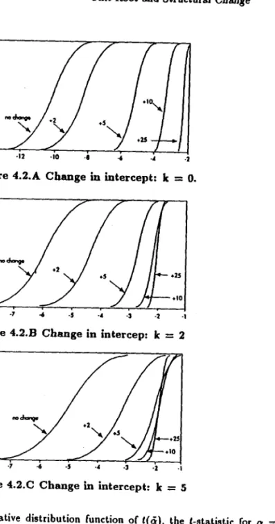
Figure 4.2 presents the results for the case of a chaoge in mean where the data are generated from (10) with I''J
=
0.2.5.10and 25 (O being the base case of no change). The graphs present the cumulative distribution functions (cdf) of the f-statistic tão
As can be seen from the graphs, the cdf of lõ is substantially shifted to the right as the change in mean increases. For k
=
O,the test has little power when the chaoge rises to 10 and none at all when the change is as high as 25 (noting that the rejection region are values of lã less than - 3.41 at the 5% levelj see Fuller (1976). These values may seem high but it is important to notice that we are considering the extreme case of a noise component that is I I D.. With a noise component positively correlated, as is the case in practice, the test no longer rejects for much lower values of the change in mean. Panels (B) and (C) show not only
'f'
li
~jfli
... ~:
~~ ~~
i30 Unit Root and Structural Cbange
I ~ ~ u ~ ~~ ~ u ~ ~I o ·lA '1> .m ~ ~ 4 ~ Figure 4.2.A Change in intercept: k
= o.
0.9 O .• 0.7 0.6 0.5 O.A 0.31 Y - ""-/ 05 I J I-025 0.2 o.ll~
.--/
/
.,r;--010 o i i , , , ·1 ·7 -6 ·5..
·3 ·2 ·1Figure 4.2.B Change in intercep: k = 2
1 0.9 0.1 0.7 0.6 0.5 O.A 0.3 O. 0.1 o ·1 ·7
...
.,
..
.,
·2 ·1Figure 4.2.C Change in intercept: k = 5 Notes:
Cumulative distribution function of t( li), the t-statistic ror o
=
1 in the regression Y,=
JJ + /3t + 0YI_I + Li=I • .I: CiÓYI_i + e,(estimated by OLS) when the data-generating process is YI=
JJ2DU, +e, (e, ,." 11 D N(O. 1) andDU,
=
1 if t > 16 and O otherwise). Simulated values are bMed 0\1 5,000 replications. The entries next to each curve are the dilTerent values of JJ2,the change in mean.
Perron 131
that this feature of reduced power remains as the autoregressive truncation lag increases but also that it becomes more severe. For k
=
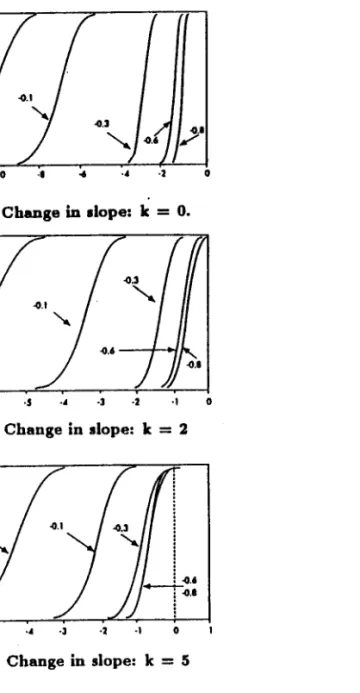
5, the test no longer has any power when the change is 5.Figure 4.3 presents the results for the case where the data-generating process involves a change in slope and is generated from equation (11) with Pl
=
1 and the changeP2 -
Pl=
O (the base case), -.1,-.3,-.6 and -.8. The same qualitative features emerge, namely substantially reduced power as the change in slope increases, more so as the truncation lag k increases. Of interest is the fact that the test looses alI power for realistic values oí the change in slope even if the data-generating process involves the extreme case of an IID. sequence. For example, with 1:=
2 the test has no longer any power when the change in slope is greater than 0.3 (in absolute value) and when 1: = 5, the corresponding value of 0.1.The simulation results described above sbow tbat tbe non-rejection of the unit root hypothesis frequently reported in prac-tice is consistent with the possibility that the processes be char-acterized by stationary fluctuations around a. trend function with a one time change in leveI andfor slope. The next section dis-cusses a different class of tests that avoids these reduced power problems and allow for the possibility of a change in the trend function.
4.5 THE TEST PROCEDURES
The test procedures are based on sim pIe autoregressions (esti-mated by OLS) that' are appropriately augmented with trend and dummy components. The test statistics are based on the values of the t-statistics for testing that the sum oí the autoregressive coefficients is equal to one. The procedures follow the approach of Said and Dickey (1984) by approximating ARMA processes by autoregressions of order k. It is important to note that the particular regression framework is different for each model and also different across the innovational and additive outlier ver-sions. The asymptotic criticaI values also differ according to the specific framework considered.
~ r
132 Unit Root and Structural Change
0.9 O •• 0.7 0.6 o. o. 0.3 0.2 0.1 1 . . / , , / ~ I o ' , , , , I I ·IA ·12 ·10 .• " ·4 ·2 o
Figure 4.3.A Change in dope: k
=
O."
"
u o 05 ~ ~ ~ u o ~ ~"
~ ~ 4 4 ·1 oFigure 4.3.B Change in alope: k = 2
1 T---~r---~~--~--~ 0.9 ;;;> 7"' 0.2 0.1
i
:i
i.a.. '--r-~.•
01 -r",-<
,../ ./,
·7 ., ·5 ·4 ·3 ·2 ·1 oFigure 4.3.C Change in slope: k = 5 Notes:
Cumulative distribution function of t(õ), the t-statistic Cor a
=
I in the regressioo !lI = IJ+
{Jt+
a!l,_.+ LI= •.•
C,ÂY,_i+
e,(estimated by OLS) when the data-generating process is li,=
{Jtt+
({J, - {J.)DT,.+
e,({J.=
1, e, '" II D N(O,I) and DT,-
=
(f - T,) iC t > T. and O otherwise). Simulated vatues are based on 5, 000 replications. The elltries next to each curve are the different vatues of the challge in the stope {J2 - {Jt."
Perron 133
4.5.1 The Innovational Outlier Modela
We start with the innovational outlier version of Models (1) and (2). The regressions, at the basis of the testing proeedures, are as follows for Models (1) and (2), respectively:
•
!lI = P + {Jt
+
-yDU, + 6D(T.). + OYI-l+
2:>IÂY.-I+
e,
1=1
and
•
(12)
111
=
P+
{Jt+
fJDU,+
rDT:
+
6D(T')1 + 0YI-l+
E
OiÂlll-i+
el (13)1=1
where we reeall that DU, = 1 and D1j = (t - T.) if t > T. (O other-wise), and D(T.), = 1 if t = T.
+
1 (O otherwise). The statistie or interest is the t-statistic (or testing that o=
1. The dummy vari-able D(T,), is introdueed (oUowing Perron (1989). In the ease where the break point T. is treated as known, it allows the t-statistie for testing o=
1 to be invariant in finite samples to the value of the ehange in the intereept under the null hypoth-esis of a unit root. When T. is unknown, sueh a finite sample invarianee property no longer holds although the statistics are asymptotieally invariant.2 In regressions (12) and (13) there are two parameters that may be unknown in practice, namely Ie and T,. We diseuss below various data-dependent methods to select them and the ensuing effeets on the eonstruetion o( the tests and their limiting distributions.4.5.2 The Additive Outlier Modela
For the additive oútlier models, the proeedures are different and eonsist o( two-step approaehes. In the first step, the trend (une-tion or the series is estimated and removed from the original
2. Note that Zivot and Andrews (1992) do not introduce the additional one-time dummy D(T,), in the regression they consider for the innovational outlier Models (1) and (2). Since this regressor is asymptoticalty negligible, this makes little dilference for moderate to targe samptes in the case where the break point is treated as unknown. We prefer to keep this dummy regressor Cor alt methods of choosing the date of break (see betow) since it naturalty extends the case oC the known break point where it altows invariance to the change in intercept under the nult hypothesis.
l
~ I.ª
~
.1 i I~ "..
.:~ , 4 -.
.
. ~ '1 :, ~ r,!134 Unit Root and Structural Change
series via the following regressions for Models (1), (2) and (3), respectively: !I,
=
IA + {Jt + 1 DU, +y,
!I,=
IA + {Jt + SDU, + l DT,° +y,
!lI=
IA + (Jt + 1 D1'; + UI (14) (15) (16)where UI is accordingly ddined as the detrended series. The next step differs according to whether or oot the first step in-volves DU" the dummy associated with a chaoge io intercept.3
For Models (1) aod (2), the test is based 00 the value of the
t-statistic for testiog that the sum of the autoregressive coeffi-cieots is equal to 1 (o = 1) in the Collowing autoregression applied to the estimated noise compooent UI :
.I; .I;
UI
=
0YI-l +E
djD(T.)I_j +E
aiÂUI-i+
e,o (17)j=O i=1
Details about the need to introduce the curreot value and lags of the dummies D(T.), can be found in Perron aod Vogelsaog (1992c). For Model (3) where no change in levei is involved and the two segments of the trend are joined at the time of break, there is no need to inlroduce the dummies in lhe second step regression. Hence, for Model (3), the secood step regression is of the form:
.I;
UI
=
aYI-l +E
aiUYI-i+
eloi=1
(18)
This two-step procedure allows a test for a uoit root that is asymptotically invariant to 1 (the magnitude of the change in
slope) under the null hypothesis.4
3. Note that the following discussion about the appropriate two-atep procedures is dilferent than that stated in Perron (1989). This paper con-Lained an error in the treatment of the additive outlier modela which ia corrected in Perron (1993) and discusaed more extensively in Penon and Vogelsang (1992c). For the case of non-trending data see Penon (1990a) and Penon and Vogelsang (1!i92b).
4. Note that such an asymptotic invariance no longer holda in the one-step procedure considered by Banerjee, Lumsdaine and Stock (1992) and Zivot and Andrews (1992). They consider a regression similar to (12) and (13) associated with the innovational outlier Models (1) and (2) ofthe form
"
Perroo 135
The construction of the test statistics of interest, namely the t-statistic for testing o
=
1 in equations (12) to (13) or (15)to (17) depend on two parameters that are in general unknown: the breu that T. and the truncation lag parameter j;. We now
discuss severai ways to choose them and the corresponding ap-propriate criticai values. Note at the outset, however, that onIy the various ways of choosing the break date influence the appro-priate asymptotic criticai values to be used, not the particular ways of choosing the truncation lag parameter.
4.5.3 Methoda to Chooas the Break Date
In some instances, the breu date T. may be treated as known or one may wish to condition lhe inference on a particular given value. In that case, one therefore needs to estimate the basic autoregressions for only one value of
T.,
that which is specifieda priori. The criticai values to be used, however, depend on the particular model selected. For Models (1) and (2) the criticai values can be found in Penon (1989, Tables IV.B and VI.B) and are the same in the innovational or additive outlier versions. For the additive outlier Model (3), the criticaI values can be found in Perron (1993). Note that the criticaI values depend on the relative position of the breu in the sample. However, unless the break occurs near the beginning ar the end of the sample, there is not much variation in the criticaI values. For this reason we only report, in Tables 4.2 to 4.6 for the various models, those corresponding to a break at mid-sample (denoted À = 0.5, with À
lhe ratio T./T).
!lI
=
IA +{Jt+1D1i +01//-1 + Li=1 •• ail/I-i +e,. The aIIympLoLic diaLribution of Lhe associated t-statiatic for o=
1 ia not invariant to the magnitude ofthe change in alope under the nulI hypotheaia. Indeed, if there ia auch a change in slope, the test will alwaya reject in large aamples irreapective of the presence or absence of a unit root in the noise component. Hence, the teat analyzed by these authors ia a joinL Leat of the null of a unit root and no change in the slope and not a teaL of the unit root hypotheaia per se where the change in slope is allowed under both the null and alternative hypotheaea. Note that even in the case where the change in slope ia zero, the asymptotic diatribuLion ia dilferent from that of the t-atatiatic associaLed with the Lwo-atep regreaaions (16) to (18).
...
I;
r
I;fi
tf
to: hjj
!~
I-o, i:r
;t
l-I,
i.i ; o.
,-I
.
;f
-.
;.
i iI .
;j :
I,
136 Unit Root and StructuraJ Change
We now consider two methods to select T, endogenously. As in Zivot and Andrews (1992), Banerjee, Lumsdaine and Stock (1992) and Perron (1990), we first consider the procedure whereby 1\ is selected as the value, over alI possible break points, which minimizes lhe t-statistic for testing a = 1 in the appropriate au-toregression. The investigator therefore needs to estimate the autoregressions for ali possible values of the break date T,o 5 The
criticaI values for the innovational outlier Modela (1) and (2) can be found in Zivot and Andrews (1992). For the additive outlier version, they can be found in Perron (1990) for ModeJ (3) and Perron aod Vogelaang (1993) for Models (1) aod (2).6 They are reproduced in Tables 4.2 to 4.6 io the lines I(a).
Ao alternative method to select the break point is, foUowiog Christiaoo (1992), to consider choosing T, as the value, over alI possibIe break points, which maximizes (or minimizes) the vaJue of lhe I-statistic for testing 1
=
O in regressions (12) to (16). This procedure imposes lhe mild a priori restriction of a one-sided chaoge in the trend fuoction. In the case of Model (1), since onIy sudden crashes are of interest for the various sedes described in Section 4.2, the procedure is to choose T, as that value which minimizes the t-statistic 00 the coeflicieot associated with thechange io iotercept DU •.
In
the case of Models (2) and (3), since only more ar less sudden increases in sIope are observed, the ioterest is in choosing 1\ as the value which maximizes the t-statistic on the coeflicient associated with DT;. the change in sJope. For aU cases, one can avoid having to make the assumption of a one-sided change by maximizing the absolute value oi the t-statistic for testing 1=
o.
For Models (1) and (3), this leads to a procedure that has properties similar to that whereby 1\ is chosen by minimizing the t-statistic for testing a = 1. For Model (2), it can lead to a substantial increase in powerj see Perron and5. Banerjee. Lumadaine and Stock (1992) and Zivot and Andrews (1992) suggest estimating the autoregressions for ali values of lhe break point in some intervaJ lhat excludes break dates near lhe beginning or the end of the sample. e.g. for ali values of T. in the intervaf (.15T •. 85T). This
makes Iittle dilference in theory or in practice.
6. Note that these papers and otbers tbat we cite below aJso report extensive tinite sample criticaJ va/ues obtained via simulations with and without data-dependent methods to select the truncation lag parameter k (see section 4.5.4 below).
PenOD 137
Table 4.2
A8ymptotic Distributioo: bmovational Outlier Model (1)
,,\=0.5 t(a) Ih) t(l11) 1.0% 2.5% 5.0% 10.0% 90.0% 95.0% 97.5% 99.0% -4.32 -4.01 -3.76 -3.46 -1.17 -0.79 -0.49 -0.15 -5.34 -5.02 -4.80 -4.58 -2.99 -2.77 -2.56 -2.32 -6.15 -4.87 -4.64 -4.38 -2.27 -1.85 -1.38 -0.70 -5.33 -5.08 -4.84 -4.59 -2.71 -2.36 -2.01 -1.54 Table 4.3
A8ymptotic Di8tributioo: lnDovational Outlier Model (2)
,,\=0.5 t(a) t(1) t (11 I) 1.0% 2.5% 5.0% 10.0% 90.0% 95.0% 97.5% 99.0% -4.90 -4.53 -4.24 -3.96 -1.96 -1.69 -1.43 -1.01 -5.51 -5.30 -5.08 -4.82 -3.25 -3.06 -2.91 -2.12 -5.28 -4.94 -4.62 -4.28 -1.64 -1.33 -0.98 -0.59 -5.57 -5.20 -4.91 -4.59 -2.15 -1.86 -1.59 -1.30 Table 4.4
Asymptotic Distributioo: Additive Outlier Model (1)
Á=0.5 t(a) Ih)
t(1"71>
1.0% 2.5% 5.0% 10.0% 90.0% 95.0% 97.5% 99.0% -4.32 -4.01 -3.76 -3.46 -1.17 -0.79 -0.49 -0.15 -5.34 -5.02 -4.80 -4.58 -2.99 -2.77 -2.56 -2.32 -4.57 -4.24 -4.01 -3.74 -1.85 -1.57 -1.34 -1.02 -4.70 -4.40 -4.17 -3.90 -2.05 -1.78 -1.52 -1.22 Table 4.5Ásymptotic Distributioo: Additive Outller Model (2)
,\ = 0.5 t(a) tC'Y) t(l-rl) 1.0% 2.5% 5.0% 10.0% 90.0% 95.0% 97.5% 99.0% -4.90 -4.53 -4.24 -3.96 -1.96 -1.69 -1,43 -1.07 -5.57 -5.30 -5.08 -4.82 -3.25 -3.06 -2.91 -2.72 -4.82 -4.54 -4.18 -3.84 -1.34 -0.96 -0.63 -0.21 -5.01 -4.71 -4.43 -4.13 -2.11 -1.79 -1.54 -1.18
Vogelsang (1993). li the one-sided change condition is imposed
a priori, the resulting procedure allows greater power. Note that in practice, for the estimation of the statistic, it does not matter if the one-sided condition is imposed or noto This dilference only affects the interpretation of the significance of the estimates.
The criticai values appropriate to these methods of choosing the break date are derived in Perroo and Vogelsand (1993) and are reproduced in Tables 4.2 to 4.6. For the case where the one-sided change is imposed a priori the criticaI vaIues are those in
..
\ :~1
~.,
1:.'
f,:
l
i:
~:,
. ! .\;
'. I iL
• 1.
jI
I
I !I
I.
I
1
,. '1 .. ! i:...
ii; .:r··
f
"': ",138 Uni& Roa' and StructuraJ Change
Table 4.6
Aaymptotic Diatribution: Additive Outüer Model (3) 1.0% 2.5% 5.0% 10.0% 90.0% 95.0% 97.5% 99.0%
.\ =
0.5 -4.49 -4.l7 -3.93 -3.65 -1.80 -1.47 -1.21 -0.85 t(a) Ih) I(hl) Notes: -4.91 -4.60 -4.36 -4.09 -2.32 -2.12 -1.97 -1.78 -4.67 -4.36 -4.08 -3.77 -1.57 -1.22 -0.90 -0.49 -4.87 -4.58 -4.34 -4.04 -2.14 -1.87 -1.61 -1.30 The sources for the asymptotic criticai values are as follows:(i) fixed .\
=
0.5, Perron (1989); (ii) 1(0), Zivot and Andrewa (1992) for Tables 4.2 and 4.3. Perron and Vogelsang (1993) for Tablea 4.4 and 4.5, and Perron (1990) for Table 4.6; (iii) Ih) and I(hl). Perron and Vogelsang (1993).the lines with the heading th). Those for the case where no such condition is imposed are in the lines with the heading t(hl)·
4.5.4 Method. to Select the Truncation Lag Parameter k
There is now substaotial evidence that using data-dependent methods to select the truncation lag parameter k leads to test statistics having better properties (stable size aod higher power) thao if a fixed k is chosen a priori unless, of course, one happens to select that value of k which is bestj see Ng and Perron (1993) and Perron aod Vogelsaog (1992a). We consider, in the empirical applications below, two such data-dependent methods. The first is the one originally implemented by Perron (1989). It uses a general to specific recursive procedure based on the value of the t-statistic on the coefficient associated with the last lag in the es-timated autoregression. More specifically, the procedure selects that value of k, say k", such that the coefficient on the last lag in an autoregression of order k" is significant and that the coef-ficient on the last lag in an autoregression of order greater than
k" is insignificant, up to some maximum order kmaz selected a
priori. In the empirical applications reported below, we use a two-sided 10% test based on the asymptotic normal distribution to assess the significance of the last lags and kmaz is set to 10.
An alternative procedure to select k is to use an information cd-terion. In our empirical applications, we report results whereby
Perron 139
k is chosen to minimize the Akaike Information Criterion (AIC).7 In the case where the noise fundion is assumed to be gen-erated from a finite order pure autoregressive processes, we cao use results in HaU (1991) to show that the two data-dependent methods described above lead to tests having the same asymp-totic distribution as would prevail if the true autoregressive order was selected to estimate the autoregression. In the case of the recursive I-statistic procedure, this holds provided kmaz is cho-sen greater than the true value. Things are more complex if we allow the (more realistic) possibility of moving-average compo-nenta in the data-generating processo This issue is investigated in Ng and Perron (1993). Qur results indicate that both proce-dures lead to the same asymptotic distribution as in the fixed k
case provided kmaz increases to infinity as the sample size (T) increases in a way 9uch that (Kmaz)3/T converges to O. However, the finite sample performances appear rather different with a moving-average component. Data-dependent methods based on information criteria, such as the AIC, tend to select very par-simonious models leading to tests with sometimes serious size distortions. This finite sample pedormaoce is consistent with our finding that the use of ao information criteIÍon leads to a selected value of k that increases to infinity, as T increases, only at rate log(T), a very slow rate. These theoretical results are in accord with the empirical results reported below for which the procedures based on the AIC lead to very small values of k
being selected (typically O or 1). This suspicion about the pedor-mance of data-based methods using the AIC is reinforced by the fact that often the estimated residuais exhibit serial correlation. These instances are indicated in the reported results. For these reasons, we put more confidence on the results obtained using
7. Among both classes considered for Lhe selection of the LruncaLion lag parameLer k, there are many other varianta that could be uaed. For example, among procedurea based on information criteria, another example
is the Bayesian Information Criterion (Ble). Since, Ble generally yielda more parsimonious modela than Ale, the same qualitative conclusioDB dis-cussed below remain. Among the clasa of procedures based on testa of significance on the coefficienta of the lag8, one could alIO use recursive joint tests assessing Lhe significance of several coefficienta on the last laga of the autoregressiona. Such procedures yielda qualitatively similar resulta as the recursive t-statistic discussed here.
,
l
I'
140 Unit Roa' and Structural Ch~ge Perroll 141
the recursive t-statistic procedure. Table 4.1
In the empirical results reported below we use the following Empirical Resulta: Real GDP Serie.
notation:
e
valuu(i) tO(t), the value of the t-statistic for testing Q
=
1 when T, isT, J:
B
;
i & t<lr CO(t) tO(aic) f'(t) t"(aic)chosen to minimize this t-statistic with J: chosen according to the (1) (2) (3) (4) (11) (li) (1) (8) (SI) (lO) (11)
recursive t-statistic on the coefficient of the last lagj Aual...u.. "ode' (3)
.
(ii) tO(aic), same as (i) except that J: is chosen according to the.782 -4.52 .03
,:-AICj 1943 2 .022 .018
[O'
~-(iii) Tl(t), the value of the t-atatistic for testing Q
=
1 when (52.89)(17.08)
;0. 1939 O .022 .018 .848 -3.52 .29
,. T, ia chosen to maximize (or minimize) the t-statiatic on 1 (the
l~
(47.04) (16.43)coefficient on the change in slope or intercept) with J: chosen
1947 2 .023 .020 .791 -4.29 .03
'. according to the recursive t-statistic on the coefficient of the last (58.71) (17.55) (.06)
I, lagj .18
,.I
1947 1 .023 .020 .844 -3.44I:
(iv) ft(aic), the same as (iii) except that J: is chosen according to (58.71) (17.55) (.31)the AIC.
t
C_.d., "ode' (3) L-.' 4.6 EMPII\ICAL APPLICATIONS .005 .615 -5.26 .04 .01 !, 1929 4 .013 -.117t
Table 4.7 presents the empirical resulta for the historical GDP se- (5.19) (-3.84) (4.50) (.02)•
.07-.... 1928 O 0.08 -.300 .003 .738 -4.43
.27-i, ries for each of the 11 countries with the corresponding model of (.14-)
;,:. (5.36) (-3.84) (3.57)
~ ! the selected trend fundion. Columns 1 and 2 give, respectively,
the date of break in the trend function and the value of the trun- D.DlDuk. MoeI.1 (3)
cation lag parameter J: in the autoregression being selected by
1938 7 .013 -.421 .004 .510 -5.94 <.01 <.01
the various methods. Columns 3, 4 and 5 present key estimated
(5.91) (-5.56) (5.42) « .01)
:
,
parameters of the autoregressions along with their t-statistics inparentheses:
iJ
is the estimate of the initial (pre-break) slope of 1938 O .008 -.282 .003 .703 -4.98 .08-.02-the trend function, Õ is the estimate of the change in the intercept (5.00) (-4.39) (4.21) (0.4-)
of the trend function in the case of Model (2), and i is the esti- Fiai_di Model (3)
mate of the change in the slope of the trend function for Models
-.327 .005 .697 -4.08 .47
(2) and (3). For Model (1) it is the estimate of the change in the 1915 3 .005
intercept of the trend function. Column 6 and 7 present the key (1.18) (-1.66) (1.17)
estimates related to the testing procedure described in the last 1912 O .010 -.037 -.001 .762 -3.93
.57-section, namely the estimate of the sum of the autoregreasive co- (2.06) (-.20) (-.30)
efficient, &, and its associated t-statistic for testing that Q
=
I, t ... 1918 6 -.013 -.729 .017 .894 -1.29.95
The last four columns from 8 to 11 present p-values associated (-2.75) (-3.47) (3.72) (> .994)
with the four different tests described earlier. As mentioned be- 1913 O .010 -.034 -.002 .769 -3.59
.27-!J
fore, these p-values are based on the corresponding asymptotic (2.21) (-.30) (-.34) (.45-)
:".;.
i: distribution of the test statistics under the null hypothesis of a (ta6le continued)
I
unit root in the noise component (allowing a break or not).
-
..
:": (f ~f:,.
-':..
, , '.
142 Unit Roat and Structural Change Perron 143
(continued from the prelliou. page) (continued from the prelliou.page)
f-lIaluu f-lIa/uet
n
IciJ
;
t
ã ta tO(t) tO(aic) P(t) fT(aic) T, IciJ
;
t
ã tá tO(t) tO(aic) P(t) P(aic)(1) (2) (3) (4) (11) (8) (7) (8) (O) (10) (11) (1) (2) (3) (4) (11) (8) (7) (8) (O) (10) (U)
... ee. Moda. (2) S_eleD' Moda. (2)
1941 9 .004 -1.28 .014 .574 -7.75 <.01 <.01 1915 9 .006 -.086 .001 .751 -4.01 .51 (6.81) (-7.56) (7.59) «.01) (4.11) (-2.72) (2.09) 1941 1 .003 -1.00 .011 .697 -6.66 < .01 <.-1 1882 O -0.01 -.047 .002 .899 -2.67 >.99 (5.72) (-6.43) (6.49) « .01) (-.27) (-2.05) (1.58) 1935 9 .008 -.147 .002 .708 -3.80 .22 Gana . . ,.. Moda. (2) (3.91) (-2.76) (2.80) (.36) 1953 1 .005 -.155 .003 .744 -4.81 .12 1905 O .003 -.033 .001 .895 -2.54 .64 (4.59) (-.927) (1.77) (2.35) (-1.58)(1.44) (.81) 1943 1 .005 -.590 .006 .750 -4.87 .20 .03 (4.65) (-3.88) (3.97) (.06) U.K •• Moda. (1) 1943 3 .006 -.632 .008 .728 -4.63 .05 1917 5 .006 -.086 .735 -5.59 <.01 <.01 (4.53) (-3.86) (3.91) (.09) (5.80) (-5,41) « .01) 1917 1 .006 -.084 .750 -.5.92 < .01 < .01 u .. ,.. Moda. (2) (6.08) (-5.42)
«
.01) 1941 1 .004 -.603 .007 .767 -4.56 .21 .06 (4.29) (-4.03) (4.15) (.11) U.S •• Moda. (1) 1944 O 4.002 -.138 .002 .855 -3.27 .90· 1928 6 .022 -.074 .693 -4.58 .11 .06 (2.86) (-1.01) (1.68) (4.52) (-3.04) (.10) 1917 O .002 -.136 .001 .910 -2.93 .50· 1928 1 .008 -.065 .766 -4.76 .06 .04 (3.13) (-2.67) (1.56) (.70·) (4.69) ( -2.82) (.06)No...". Moda. (3) Notes:
1941 3 .022 .020 .848 -3.18 .48 The last four columns report p-vaJues as80ciated with the t-atatistic ta for (57.75) (21.80) testing a
=
1 in the appropriate regression model denoted in the second 1944 O .022 .021 .876 -2.84 .68 column. tO(t) and tO(aic) refer to the p-vaJues associated with choosing T, (63.01) (22.30) minimizing tá. The former chooses l: uaing the recuraive t-statistic procedure 1945 O .022 .021 .877 -2.84 ,42 and the latter chooaes l: uaing the AlG; P(t) and P(aic) refer to the p-valuea (64.68) (22.41 ) (.63) &saocÍated with cho08ing T, maximizing the t-atatiatic on the coefficient 1945 1 .023 .021 .871 -2.85 .42 of the change in alope for Modela 2 and 3 (or minimizing the t-statiatic (64.68) (22.41) (.63) on lhe coefficient or the change in intercept in the case or Model 1), the former cho08es Ic uaing the recuraive t-atatistic procedure and the laUer(ta6/e continued) uses the AlG. The main entries correapond to one-tailed test and those in parentheses to two-tailed testa (i.e. without imp08ing a priori the sign or the change in slope). An entry with a • indicates that the residuais from lhe estimated equation exbibited aignificant serial correlation according to the Box-Pierce statistic.