Carlos Pestana Barros & Nicolas Peypoch
A Comparative Analysis of Productivity Change in Italian and Portuguese Airports
WP 006/2007/DE _________________________________________________________
Andrea Gavosto, Guido Ponte and Carla Scaglioni
Investment in Next Generation Networks and the Role of
Regulation: A Real Option Approach
WP 031/2007/DE _________________________________________________________
Department of Economics
WORKING PAPERS
ISSN Nº0874-4548
School of Economics and Management
Investment in Next Generation Networks and the Role
of Regulation: A Real Options Approach
#Andrea Gavosto, Guido Ponte and Carla Scaglioni
Economic Research Division - Telecom Italia∗
Preliminary
This draft: 11 December 2007
Abstract
The current regulatory debate in the telecommunications industry in Europe and elsewhere
is dominated by the issue of if and how to regulate next generation networks (NGN) which
operators plan to roll out in the near future. The crucial issue is whether an extension of
current regulatory obligations onto future networks would hamper the investment by large
European operators. The paper applies a real option model to explain the investment
decision in next generation networks. One important result of the model is that regulation
affects the investment decision only in the initial period when uncertainty is still very high.
The real option model has been calibrated with parameters drawn from real data for a new
entrant and from educated estimates for an established operator. Four different regulatory
regimes and their impact on the timing of the investments have been simulated: a temporary
regulatory holiday is shown to be an effective regulatory tool in order to induce immediate
investments.
JEL Classification Numbers: L51, D81, G11, G35
Keywords: real options, telecommunication, regulated industries, Next Generation Networks.
#
The opinions expressed herein are those of the authors and do not necessarily reflect those of Telecom Italia. We thank Íñigo Herguera and the partecipants to the IDEI/Bruegel Conference, 25-26 October 2007-Brussels, on Regulation, Competition and Investment in Network Industries for useful comments
∗Strategy-Studi Economici. Corso d'Italia 41, 00198 Rome. Corresponding author:
Contents
1 – Introduction ... 3
2 – Regulation and Investment... 4
2.1 – The next generation networks... 4
2.2 – Literature review... 8
3 – A real option theory approach to the telecommunication industry ... 10
3.1 – A discrete binomial model: an illustrative example ... 10
3.2 – Impact of regulation on investment: the issue of truncation... 19
4. – A model to evaluate investment in NGNs. ... 22
4.1 – Model input parameters ... 23
4.1.1 – General inputs... 25
4.1.1.1 – Citéfibre specific inputs... 25
4.1.1.2 – Established telecommunication operator inputs ... 27
4.2 – Model outcome and the role of regulation... 29
5 – Concluding remarks ... 39
1 – Introduction
The current regulatory debate in the telecommunications industry in Europe and
elsewhere is dominated by the issue of next generation networks (NGN). The term refers to
the installation of high-speed physical infrastructures, largely based on optical fibre, and to
the use of platforms based on IP (Internet Protocols) for the transmission of integrated
services for voice, data and video. Under many respects the NGNs represent a dramatic
technological shift in the provision of telecom services: new networks enable a bandwith up
to 100 megabits per second, as compared to the maximum of 20 megs currently available
on DSL platforms. On the other hand, NGNs require massive investments by telecom
operators, of the order of several billion euros in a single country, in the face of a
widespread demand and regulatory uncertainty. Demand uncertainty arises because the new
networks are instrumental to a host of new services for residential and corporate customers,
such as Internet TV, e-government, e-health, e-learning and so on, whose acceptance with
final customers is still to be ascertained. Regulatory uncertainty arises because, at this
stage, it is still unclear whether regulators are going to carry over current obligations on
traditional services to NGNs or to apply more lenient rules – even, possibly, a regulatory
forbearance as in the US - taking into account that, differently from traditional networks
built at the time of the state monopoly, NGNs do not exist yet. A summary of the regulatory
debate in Europe will be provided below. Investment in NGNs has been relatively subdued
until now: operators want to know the future regulation of NGNs and to have a better guess
of demand perspectives, before committing a vast amount of resources to the new
networks.
This paper purports to examine the investment decision in NGNs by telecom operators,
in the light of high demand uncertainty. To do so we exploit the real option theory, which
allows us to include the postponement of investment among the options available to firms.
Once the base case is defined and calibrated, different regulatory solutions will be analysed
The paper is organised as follows. In section two we give a brief overview of regulation
and investments, notably by providing stylised facts for the next generation networks and a
review of the literature. In section three we explain how real option theory works. Section
four describes the model employed to test the impact of different regulatory regimes on
investments in next generation network and discusses regulatory options. Section five
provides our conclusions.
2 – Regulation and Investment
2.1 – The next generation networks
In the OECD countries (OECD, 2007), investments in telecommunication networks has
been characterised by a record growth in the period up to 2000 and by a subsequent strong
decrease, from a value of USD 243 billion in 20001, which includes investment in tangible
infrastructures2, to below USD 160 billion in 2005. Such a decrease was mainly due to two
factors: i) the end of the massive initial investments in access and backbone infrastructures,
both fixed and mobile, by new entrants in the telecommunication market, led by
over-optimistic expectations on the pick up of Internet services; ii) the end of the financial
bubble in the telecommunication industry, that pressed operators and capital markets to be
more focused on obtaining an adequate return on investment3.
1 Corresponding to more than three times the total investment in the sector a decade earlier. The figure
includes auctions for licences to spectrum allocated for 3G (UMTS, IMT-2000) services for most of the European countries, with the exceptions of Denmark, Greece, Luxembourg, Poland and Sweden.
2
Following OECD (2007), the main drivers for this raise in investments were construction of second generation wireless networks, the entry of new competitors into local access markets for fixed networks, and very large commitments by new entrants and incumbents in national and international backbone infrastructure.
3
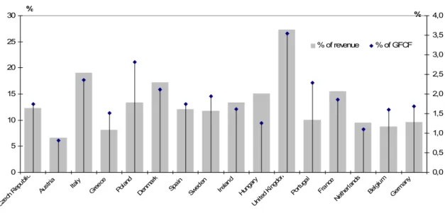
Figure 1 –Public telecommunication investment as a percentage of PTO revenue
and gross fixed capital formation (GFCF)
(2005) 0 5 10 15 20 25 30 Cze ch R
epubl ic Aust ria Italy Greec e Pol and Den mar k Spai n Sw eden Irelan
d Hunga ry Uni ted Kingd om Por tuga l Fran ce Net her land s Belg ium Ger man y % 0,0 0,5 1,0 1,5 2,0 2,5 3,0 3,5 4,0 %
% of revenue % of GFCF
Source: adapted from OECD (2007).
The slowdown in investment that dates back to the beginning of the decade is probably
coming to an end. On the one hand, the excess capacity that has characterised the decade as
a consequence of the massive build-up of transmission infrastructures from 1995 to 2000 is
finally being eroded by the dramatic increase in demand for broadband Internet4.
Broadband connections all over Europe have jumped from 52.6 million in 2005 to over 70
million in 2007 (European Commission, 2007a). On the other hand, the technological
paradigm is shifting. Differently from the leading ADSL technology, where traditional
analogue voice services and digital data transmission for Internet run over two different
platforms, in next generation networks voice (typically, voice over IP), music, videos and
all other sort of data are transported over the same integrated network.
4
NGNs will increase bandwith (i.e. the ”speed” of the Internet connections) dramatically,
up to 100 megabits per second, which will enable transmission of several channels of high
definition television and services such as e-government, e-health, e-learning and so on.
Therefore, the next generation networks will be the leading driver of the future investment
in telecommunication networks. The European debate mainly concerns the deployment of
NGNs at the access (i.e. local loop) level: in this paper we will concentrate on access
NGNs.
Laying fibre up to the customer’s premises or close to it represents a serious financial
effort, mainly due to the cost of obtaining building permits and of engineering works in
urban and rural areas, which together represent from 50 to 80% of the overall capital
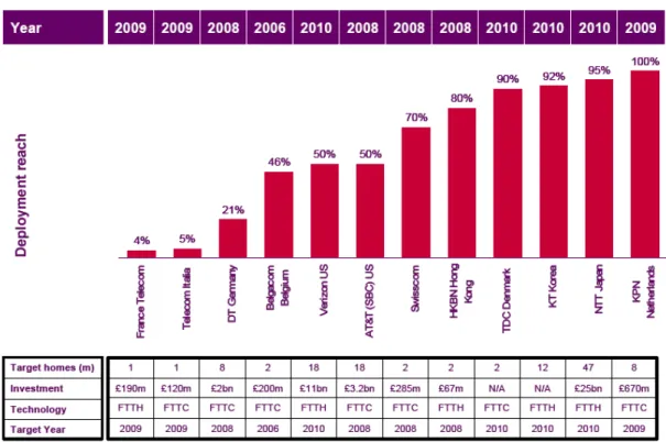
expenditure5. So far, the main European operators have announced preliminary plans of
investment (see Figure 3). In Italy, Telecom Italia expects to invest between 6 and 7 billion
euros in next generation networks by 2015. Such an effort will be tuned according to the
increase of demand for services based on NGNs.
Next generation networks have the potential to offer substantial economic benefits. They
can:
• lower substantially operating costs, (instead of several networks, each with its own
provisioning and maintenance procedures, a NGN carries all traffic on a single
network);
• allow operators to develop services more quickly and more cheaply because
intelligence is centralised rather than embedded in switches, (this in turn allows
them to experiment with services to find out which ones best meet end user needs);
• deliver higher functionality services, (because of their ability to integrate and
bundle services).
In other words, NGNs can both lead to cost savings in the provision of services and
Figure 3 –Incumbent next generation access deployment plans by target date
Notes: in euro terms the amounts for each operator are: FT €273m, TI €172m, DT €2,8bn, Belgacom €287, Verizon €16bn, AT&T €4,5bn, Swisscom €409m, HKBN €96m, NTT €36bn, KPN €962m.
Source: adapted from Ofcom (2007).
The pace with which these potential benefits are realised will clearly depend on how
NGNs are regulated. The regulatory question for NGNs is quite well defined (its solution
less so, as we will see). Differently from the usual regulatory problem in
telecommunications – that is the opening up to competition of a legacy infrastructure, the
copper network, built during the monopoly years – the question here is how to define future
rules for networks which do not exist yet. The relevant trade off is between the incentive to
investment and the degree of competition in the future telecommunication market. On the
one hand, in fact, established operators, which will, inevitably, sustain most of the
investment in several countries, are waiting to see whether regulatory authorities decide to
5
impose permanent regulation6 wholesale obligations on the next generation networks, such
as the ones which exist presently on traditional networks: typically the obligation to provide
access to the established operator network elements (for instance, the local loop) at a price
which corresponds the full distributed cost of the service, as recorded in the regulatory
accounting. If this were the case, one could surmise that established operators face fewer
incentives to build NGNs, as regulation will immediately wipe out the quasi-rents arising
from the deployment of new infrastructures. Symmetrically, the existence of wholesale
obligations, and their scope, will also condition the behaviour of the new entrants, which
may either decide to make major investments or to exploit the established operators' NGN
as the latter are gradually installed (free riding behaviour), thus side-stepping significant
fixed costs.
On the other hand, regulatory bodies are concerned about removing any initial
conditions of major advantage to the established operator that could preclude the
development of a competitive market. The potential advantages are represented, on the one
hand, by the exclusive availability of some network elements (such as reconnections from
the cabinet to the user's premises or the ducts in which to install the fibre); on the other
hand, by the control of an initial customer base which could enable the established operator
to reach significant network economies before its competitors. For these reasons, regulators
such as the European Commission are quite hostile to regulatory forbearance and regulatory
holidays, that is the absence of all obligations on NGNs for at least a pre-defined period of
time, as imposed by the German telecommunications bill (and fiercely opposed by the
Commission)7.
2.2 – Literature review
In highly capital intensive industries the launch of a new service or a technology often
involves lumpy investments. Such investments are not necessarily carried out at the time
when the investment opportunity arises, even if they are profitable (in the sense that they
6
As we have defined it at page 33.
7
would produce a positive discounted cash flow). Often investment opportunities are held
“on the shelf”.
It is generally agreed (Guthrie, 2006) that one of the main reason for this delay is the
nature of the regulatory framework. Accordingly, economic literature on the impact of
regulation on investments is divided into two areas of research: (i) standard investment
analysis where the impact of regulation (either rate-of-return or incentive regulation) is
usually evaluated in a static context, although occasionally dynamic models of investment
behaviour8 are applied; and (ii) real options approach.
Several authors have focused their attention on the realistic rate of return for a regulated
firm but none has been able to find a solution in the case of firms which undertake
irreversible investments while constrained by incentive regulation with periodic retunes9.
Other authors have integrated uncertainty and irreversibility in their models and have
considered the more general problem of setting regulated prices when faced with
non-constant demand and technology10. Beard et al. (2003) employ a two-period model in
which a regulator decides (i) the revenues which a firm is authorized to earn in the case that
its assets are not stuck, and (ii) the reward which the firm will obtain if its assets are
stranded. The less reward offered, the more profit must be allowed if the firm is to
voluntarily invest in the project. As a result, full compensation would not be given by a
welfare-maximizing regulator.
Conversely the real option approach captures the notion that, in the real world, demand,
technology, factor prices and other parameters affecting investment decisions are subject to
many uncertainties11. As a consequence it may be in the company’s own interest to delay
the investment in order to acquire more information and ultimately to reduce risk. In
8
A survey of the static and dynamic models of investment under different forms of regulation and optimal (Ramsey) pricing may be found in Biglaiser and Riordan (2000). Most of this literature assumes static models of which the Averch-Johnson is the best known (1962). These models show that rate-of-return regulation does not provide the incentive for the firm to minimize costs or capital investments.
9
Evans and Guthrie (2005) provide en exstensive review of the topic.
10
Dobbs (2004) estimates the firm’s choice of the level and timing of investment when constrained to a price cap which is proportional to the established capital price; that is, the cap varies with the replacement cost of the firm’s assets.
11 The literature on real-options research from the financial perspective is reviewed and integrated in
particular, in these models, regulation can restrict the flexibility of the firm through the
introduction of constraints on prices and on costs associated with delay, abandonment, or
shutdown/restart options.
Although investment decisions in the telecommunications industry often involve
both irreversibility and uncertainty, a limited literature exists on the application of real
options to the telecommunications industry12.
In this paper we extend McDonald and Siegel (1986), who initiated the theory of
irreversible investment under uncertainty in a continuous time setting – later extensively
developed by Dixit and Pindyck (1994) –, by considering investments which have finite
lifespan, whose length is known in advance. Also we use a discrete time setting rather than
the continuous one employed by McDonald and Siegel.
In the next sections, we will present an illustrative example of the decision process of
firm according to real option theory; subsequently we will describe our model and apply it
to NGNs; finally we will compare the impact of different regulatory regimes onto
investments.
3 – A real option theory approachto the telecommunication industry
3.1 – A discrete binomial model: an illustrative example
In this section we present an illustrative example with the aim at making the reader
acquainted with the reasoning behind the optimal exercise of an option. We also introduce
the concept of critical values (i.e. prices above which the option holder should rationally
exercise the option) and examine how do these values vary in response to a change in the
12
model inputs (stock volatility, risk free interest rate, pay out ratio, option lifespan, etc).
Finally, we develop the parallel between a financial option and a business opportunity and
we examine how it works in a discrete time setting.
The example is framed within a discrete multiplicative binomial event tree. Differently
from models in continuous time, such as those by Black and Scholes (1973) and Merton
(1973), a discrete setting helps to clarify the economic principles underlying option pricing.
The logic that lies behind the solution of discrete time problems and that of continuous time
problems is exactly the same: often solutions to continuous time problems are found by
converting them into equivalent discrete settings. The numbers in this example are chosen
to make computations simpler, but nothing of substance is lost.
Let us consider a 3-year time horizon (see Figure 4). At time t=t1, there are two possible
states of nature (“Up” and “Down”); at t=t2, there are four possible states of nature (“A”,
“B”, “C” and “D”); finally at t=t3 there are eight possible states of nature (“1”, “2”, “3”,
“4”, “5”, “6”, “7” and “8”).
Let us suppose that a firm can choose between a risk-free security, worth 1,000$, which
earns 3% per annum, and an investment project which requires a 480$ disbursement, and
whose expected net cash flow are equal to 500$ (again, the numbers are chosen for the sake
of simplicity). The investments opportunity ceases to exist at t3 i.e. three periods after the
investment opportunity arises.
The firm opportunity to invest can be thought as a call option on a stock whose price
evolves following the same stochastic process as the expected net cash flow. The strike
price, worth 480$, is equal to the up-front disbursement required to implement the
investment and is exogenously given. The financial equivalent of the last date at which the
investment can be carried out (i.e. t3) is to be considered as the option expiry date.
Let us now look at the cost associated with keeping the investment opportunity at bay
for one period: each year of delay implies less payout (extra revenues and cost savings) to
stock is the dividend periodically paid by the company to its shareholders13
. In the example
we assume that the payout is a fixed percentage (10%) of the net present value of the
project at the different nodes (in financial terms, this would correspond to the stock price).
At each node the company can either invest 480$ (exercise the option by paying the
strike price) and receive the project NPV14 (one share of the company) plus the period
payout15 (the dividend) or, conversely, it can decide to postpone the beginning of the
investment to the next date (hold the option unexercised). The company decides what to do
after the state of nature has revealed itself (i.e. the company knows how much the net
present value is worth at that date). We suppose that at t3 the business opportunity ceases to
exist and thus t3 represents the last chance the company has to start the project (to exercise
the option).
We can now describe the company decision process, as illustrated in Figure 4. Each
node of the binomial tree is identified by an array of seven numbers. In the first row, we
indicate the business opportunity value and whether it is optimal to undertake the
investment (grey area) or not. In the second row, first column, we represent the NPV of the
project; in the second column, the payout of the project, i.e. the extra revenues and cost
savings, at the current date. In the third row, first column, we show the value of the risk free
security; in the second column, the period project payout. In the third row, first column, we
show the value of the risk free security; in the second column, the state prices of the project
payoff which encompass all future information on the states of the nature. Finally, the
fourth row includes the value of the business opportunity if not exercised (first column) or
exercised (second column): clearly, the value of the option is the greater of the two.
The market formed by the risk-free security and the project allows no arbitrage and it is
dynamically complete. Under no arbitrage a set of state prices exist; due to market
completeness, it is also unique. We can thus price all contingent claims by the no arbitrage.
13
In the case of a NGN deployment the incremental revenues and cost savings (i.e. the investment payout) corresponds respectively to the extra revenues arising from, say, TV on Internet plus the cost savings – mainly in terms of less maintenance and provisioning - induced by the replacement of the current copper access with NGNs.
14
The NPV of the project is equal to the sum of the payouts from the next date to the date the projects ends.
15 T
At t0 the value of the project, denoted by S, is assumed to be equal to 500$. In the
following period, t1, following the multiplicative binomial stochastic process, the NPV of
the project can either go up by 60% to St1=St0 *(1+0.6) or go down by 20% to St1=St0
*(1-0.2). At t2 the NPV can either go up to St2=St1*(1+0.25) or go down to St2=St1*(1-0.15).
At t3 the stock price can either go up to St3=St2*(1+0.1) or go down to St3=St2*(1-0.1).
Note that in the example the range of the price changes in each node is chosen to make
calculations simple. However it is greater (in absolute value) at the beginning of the project
than at the end (60%, -20% versus ±10%) in order to capture the idea that as information
flows in with time, demand uncertainty falls, and hence the project becomes less risky
while earning a constant return. In fact the payout ratio (i.e. the ratio between the one
period payout and the NPV) is kept constant through all the project lifespan.
How do we compute the values of the option whether it is exercised or not at each node?
If it is exercised, the value of the option, shown in the orange cell (fourth row; second
column), is equal to the sum of the current NPV plus the period payout minus the option
strike price. If it is not exercised, the value of the option, shown in the green cell (fourth
row; first column), is equal to the next period payoffs (associated with adopting the optimal
exercise policy) times the state prices16. The American call option value, contained in the
blue cell, is equal to the greater between these two values.
What is the intuition? If the option is exercised, i.e. if the investment is made in the
current period, the company will gain the extra revenues and lower costs linked to the
immediate investment (the payout) plus the value of the project in all future periods, as
captured by the NPV. In exchange, the company has to pay the strike price: for instance,
the cost of deploying fibre in the access network. On the other hand, if the option is not
exercised at tn, i.e. the investment has not been yet carried out, its value is a function of the
payoffs at tn+1, associated with the optimal exercise policy across all future states of nature.
In order to compute the value of the option when not exercised, one has to work backwards
through the binomial tree, determining at each node whether or not it is optimal to exercise.
16
Figure 4 –Binomial event tree
t=t0 t=t1 t=t2 t=t3
“1” 675
Node “A” 1100 55
1092,7 0,39
570 0 675
1000 50 675
1060,9 0,32 “2”
Node UP 534 570 465
534 900 45
1092,7 0,58
360 0 465
800 40 465
1030 0,22 “3”
334 360 305
334 Node “B” 748 37,4
1092,7 0,39
234 0 305
680 34 305
1060,9 0,65 “4”
214 234 163
Node t0 214 612 30,6
1092,7 0,58
90 0 163
500 25 163
1000 “5”
90 45 98
89,8023 Node “C” 550 27,5
1092,7 0,39
45 0 98
500 25 97,5
1060,9 0,32 “6”
38 45 0
Node DOWN 38,3 450 22,5
1092,7 0,58
14 0 -8
400 20 0
1030 0,75 “7”
14 -60 0
14,3 Node “D” 374 18,7
1092,7 0,39
0 0 -87
340 17 0
1060,9 0,65 “8”
American call option value 0 -123 0
Stock price Payout 0 306 15,3
Bond price State price 1092,7 0,58
Let us begin from the final period. If the option is still not exercised at t3, then the
optimal policy is as follows: to exercise if the sum of the NPV and the payout (i.e. the
payoffs obtained by exercising) exceeds the strike price; not to exercise, otherwise. Once
the payoffs at t3 (associated with the optimal exercise policy) are known, the value of the
option at t2 if not exercised can be computed by backward induction. At t2 the optimal
exercise policy is to exercise if the value of the payoffs received by exercising (payout +
NPV) exceeds the value of the unexercised option. By applying the same backward
induction we can find the American option value at all previous nodes.
To better understand the difference between the value of the option to invest when
exercised and when it is not, we can be decompose it into three components17. The first is
the “lost payout”. When the option has been stroke early, say at tn, the company collects the
payout (incremental revenues and cost savings) arisen at tn. If instead the company holds
the option for one extra period, it loses the payout at tn. On the other hand, by holding the
option for one more period, the company benefits from the postponement of the cash
out-flow: this is the second component. The third component is given by the value associated
with protracting the period in which it is possible to choose between the two alternatives: in
fact at the subsequent nodes the value of the unexercised option may still exceed the
payoffs (payout + NPV) gained by exercising. We will refer to this component as the
“reversibility component” which adds to the value of the option when not exercised. At the
date prior to expiry (i.e. t2) the company avoids incurring losses at expiry by postponing the
decision to invest. This is why in this case the reversibility component is referred to as the
protection value
We can now define the decision rule: an American option is rationally exercised when
the value of the payout exceeds the interest cost associated with an early disbursement of
the strike price (the “cash-out postponement”) plus the loss of the insurance against the
possibility that payoffs at expiry are less than the strike price (the “reversibility or
protection value”). In other words, according to the real option model, the investment is
carried out when the revenues gained from having implemented the project exceeds the
financial benefit due to the fact that the up-front disbursement investment cost (cash
outflow) becomes smaller in present value terms.
If volatility is zero or if all possible payoffs at expiry are above the strike price, the
insurance component is obviously worth zero, and thus it is optimal to defer the exercise of
the option as long as the interest savings exceeds the lost payouts. For example at the UP
node of the event tree, the value of the cash outflow deferment is equal to 14.4 (480$ times
the exogenous interest rate of 0.03), whereas the payout is equal to 40. Thus the benefit of
exercising exceeds the cost and the option is rationally exercised.
In order to illustrate the decision process on whether to exercise or not it is useful to
compare node t0 and node “C”. In fact, at these two nodes the NPV and the payout are the
same; still, as we will see, in the latter case it is optimal to exercise the option while in the
former it is not. In our example, the rate of interest is kept constant over the event tree,
hence the cash postponement component is exogenously given and the same at both nodes
(see Figure 5 and 6). Equally, the lost payout is the same by construction. All the difference
is thus given to the reversibility-protection component. In particular, at node t0 the
reversibility component is higher because the array of possible outcomes (payoffs at expiry
prices) is much greater than those which can be reached from the node “C”: hence the value
of the insurance against “bad” states of nature is much greater. At node “C” the range
possible final payoffs decreases substantially since, as time elapses, some final outcomes
can no longer be reached and the rate of change of prices at t2 (± 10%) is much smaller than
at t0 (+60%; -20%). In a continuous time setting this is equivalent to saying that the total
variance falls with time because the time horizon becomes shorter and the variance per unit
of time decreases. In conclusion the optimal strategy is not exercise at t0 but to exercise at
“C”.
17
Figure 5 –Decomposition of the option value at node t0
Value of the four components of the unexercised option at node t0
45
14
56
90 -25
0 20 40 60 80 100 120 140
Option payoff if exercised
Cash outflow postponement
Reversibility Lost dividend Option value if
unexercicesd
Figure 6 –Decomposition of the option value at node “C”
Value of the four components of the unexercised option at node C
45
14 4
38 -25
0 20 40 60 80 100 120 140
Option payoff if exercised
Cash outflow postponement
Reversibility Lost dividend Option value if
The cash outflow postponement component assumes the same value at t0, t1 and at t2
while it is zero at t3 (at expiry the cash outflow cannot be postponed any longer). Moreover
it is independent from the project value. The reversibility component decreases with time
and at any date tn it is a monotonic decreasing function of the value of the project.
Conversely the opportunity cost (lost payout component) is independent of time, whereas it
linearly increases with the value of the project.
A simple argument establishes that at any tn the optimal stopping policy can be
expressed in the following terms: exercise if Stn>S*tn; do not exercise otherwise. The
optimal stopping rules reflects the intuition that when the stock price is sufficiently high the
probability of incurring losses at expiry is quite low (low protection) while the lost payout
due to because of waiting becomes significant (high opportunity cost).
Since the value of protection falls with time, the critical values S*tn, above which it is
optimal to carry out the project, decreases as the date of expiry becomes closer (see Figure
7).
Figure 7 –Critical values S*t0, S*t1, S*t2 and S*t3
Exercise area
Continuation area
437 489
537 604
0 100 200 300 400 500 600 700
3.2 – Impact of regulation on investment: the issue of truncation
The example of the previous section allows us to highlight one important result of the
real option model as far as the impact of regulation on investment is concerned: the fact that
the expectation of future regulatory remedies does not tilt the investment decision by the
company. This is known as the ‘truncation’ issue.
As we stressed earlier, the central theme of the regulatory debate is whether existing
obligations, which basically consists of granting access to the established operator’s
network at prices equal to costs, can be extended onto future networks without causing the
investment in NGNs to be reduced or even cancelled. The leading view by large operators -
which has been represented by LECG (2007) in a paper made for the organisation of
incumbent operators - is that an extension of current obligations would lead both
incumbents and alternative operators to reduce the amount of investment in NGNs.
Established operators would cut back on investment because regulation will make
perspective quasi-rents to disappear; on the other hand, alternative operators would rather
buy the services from incumbents at regulated prices than make their own infrastructures.
Such a view is echoed by Ofcom, the UK regulator, in a recent document on NGNs:
“The imposition of regulatory remedies that mandate access at a specific price may result in
asymmetric risk borne by investors and a change to the prospective returns available for an
investing firm. .…. However a straight-forward application of the standard cost plus pricing
approach may result in lower incentives to invest. This approach would cap the total returns
that the firm could make if demand turned out to be high but force the firm to bear all of the
losses in the event that there was virtually no demand” (Ofcom, 2007).
Whereas the reasoning by Ofcom is well grounded in traditional finance models, such as
the capital asset pricing model, in a real option context this view needs to be qualified.
Regulatory intervention that caps the total returns affects investments in NGN negatively
only in the initial period; in the long run, according to the real option model, investments
are not affected.
In order to understand this point, we have to go back to the illustrative binomial example
possible NPVs, i.e. the present value of cash flows from the expiry date onwards, which
will arise at the expiry date of the option which we assumed to be t3. As we move from t0 to
t3, the spread of the expected distribution of the NPVs at t3 becomes smaller, as uncertainty
on the project outcome wanes (and the value of reversibility is reduced as a consequence).
By the time we reach the expiry date, t3, there is hardly any uncertainty left: the distribution
collapses to a single value of the net present value of the project, which we assume to be
known. As we described earlier, the decision rule is that, if at t3 the present value of cash
flows onwards (NPV) exceeds the strike price, then the investment is carried out; otherwise
the investment is waived for ever (see Figure 8).
Now let us suppose that the regulator decides to cap the company’s returns by imposing
a cap on the overall project rate of return from the expiry date onwards. This amounts to
prevent the company from earning the excessive payoffs, i.e. to truncate the right-hand tail
of the distribution at the expiry date. As Ofcom correctly points out, the expected return for
the company falls under regulation. Does this tilt the decision whether to invest in our
model or not? It does not. In fact, in real option models the company decision to invest is
exclusively affected by the shape of the distribution below the strike price and not by the
shape above the strike price.
Except in the (very unlikely) case that the regulator imposes a rate of returns cap
permanently below zero (i.e. cumulative net cash flow falls below the investment
disbursement) – that would cause the company to run consistent losses -, the portion of the
NPV distribution which lies below the strike price remains unchanged even after the
truncation imposed by the regulator: hence the incentives to invest are unaffected. Thus
over the long run, that is from the expiry date onwards, the investment decision by the
company is unaffected by a rate of return cap18, at least within this real option model.
This result holds true from t3 onwards. In the initial period, from t0 to t3, when
uncertainty over the project outcome still exists, the intervention of the regulator does make
a difference, however. In fact, by lowering the payout, the regulator tilts the decision of the
company on whether to exercise the option or not by affecting the “lost payout”
component. Obligations from the regulator make it more likely that the company postpones
its investment decision until t3. As we shall see, this finding supports the regulatory
prescription of relaxing regulation on NGN in the initial phase of the investment when
uncertainty is still high.
18
4. – A model to evaluate investment in NGNs.
This paragraph aims at identifying a model for evaluating call options for which
premature exercise may be optimal, which captures best the characteristics of the
investment in next generation networks by telecommunication operators19.
In order to apply a real option approach to investments we assume the existence of an
asset or of a dynamic portfolio of assets which is perfectly correlated with the investment
net cash.The firm’s ability to defer an irreversible investment is akin to an American call
option. The financial option parallel arises from the fact that the firm has the opportunity -
but not the obligation - to undertake an investment at some future moment in time.
In real life managers evaluate investments opportunities on a monthly or quarterly basis.
Therefore, models which allow the exercise of the option (and the evaluation of its
optimality) at a certain pre-specified (equally spaced) dates reflect business reality better
than those framed in continuous time settings: these are known as Bermudan options, since
they lie in between American options (which can be exercised continuously) and European
ones (which can be exercised only at expiry).
In the telecommunication industry, there is still an enormous uncertainty surrounding the
returns on services based on NGNs, as stressed at the outset of the paper. Clearly such
services cannot be the same as the current ones based on DSL or similar technologies: if
this were the case, there would be little point in incurring a massive disbursement such as
the one required by NGNs, whereas operators could upgrade their network incrementally in
order to reach higher speed and better quality of service20. Hence NGN services and their
prices are still clouded by a vast amount of uncertainty.
Based on past experience, the main uncertainties regarding the project revenues and cost
savings would typically unveil themselves within five to seven years from the emergence of
the business opportunity. After a certain number of years, the volatility can become so
19
In the last decades the literature on financial option focusing on valuing call options for which premature exercise may be optimal has been abundant. For a brief presentation of the various techniques and approaches available see Gekse and Shastri (1985).
20 In certain areas where the telecommunications copper network encounters serious bottlenecks or congestion
small that it no longer affects the overall profitability of the projects. This implies that
optimal “now or never” decisions are taken before expiry21. When the volatility of the
project becomes negligible, the reversibility component tends to zero and the remaining
lifespan of the option does not affect the optimality rule computed at the previous nodes. In
order to model business opportunities whose volatility disappears after a certain number of
years, we make use of finitely lived options.
The Cox, Ross and Rubinstein (1979) model lends itself to be employed for finitely
lived Bermudan options. It discretises both time and price changes through a recombining
symmetric binomial tree. The distribution of dividends and price changes occur at discrete
time intervals. Due to the recursive structure of the problem the solution is obtained
through iteration.
In the following we will test the model first by applying it to a new entrant operator that
decided to invest in FttH technology back in 2005; then to an established operator, which
has to decide whether to invest in NGNs on the basis of a number of educated guesses on
revenues and costs22.
4.1 – Model input parameters
TheCox et al. (1979) model requires the following parameters:
• current expected net present value of the project, denoted by NPV
• up-front investment, denotes by UI
• net cash flow lost by a one year postponement of the project
commencement date, denoted by PO (Pay Out) ;
• annualised logarithmic volatility of the project returns, denoted by VOL
(Volatility);
• risk free rate, denoted by Rf;
21
An optimal “now or never” decision is a one whose optimality remains unchanged over time.
22
• number of years after which the sign of the overall project profitability
ceases to be a stochastic variable (i.e. years to expiry), denoted by YtE
The model outcomes (option pricing, optimal timing, optimal policy) are homogeneous
of degree zero with respect to NPV and UI. This allows to establish the optimality of
investments on the basis of the profitability of a single NGN connection. The VOL variable
measures the standard deviation of the natural logarithm of projects returns (i.e. ratio of
NPV at tn to NPV at tn-1). The PO variable is expressed as percentage of NPV.
In order to define the VOL parameter, i.e. the NPV annualized volatility, we need to rely
on the existence of a NGN pure player which is traded on an exchange market. We have
decided base our calibration on Citéfibre, a small scale fibre-to-the home Parisian operator.
Citéfibre was established in October 2004 and it was floated on the EuroNext Paris
exchange on the 2nd December 2005. After the signature of an agreement with the
Municipality of Paris in the beginning of 2005, Citéfibre began the actual fibre rollout in
the second half of 200523.
In our simulations the initial phase of the project life, the one surrounded by uncertainty,
is assumed to last for six years. The parameters of the model can be separated in two
categories: general inputs and operators’ idiosyncratic inputs. The risk-free rate and years
to expiry are both general inputs to the model, while the remaining parameters depend on
the characteristics of the specific NGN investment plan (either new entrant’s or established
operator’s).
23
4.1.1 – General inputs
The risk-free rate is assumed to be constant and equal to 5.5% over the first phase of the
project. The risk-free rate corresponds roughly to the average cost of money in Europe over
the past twenty years.
The number of years after which main uncertainties disappear is assumed to be six years.
This is the average time lag between when the front-runner European telecommunication
operator adopts a new technology and when the last follower introduces it. The project time
optimality is evaluated every quarter.
4.1.1.1 – Citéfibre specific inputs
The actual fibre roll-out of Paris by Citéfibre began in the second half of 2005: this is the
date when the investment opportunity was irreversibly converted into a business plan. We
make use of the standard hypothesis of rational expectations: as a consequence, we assume
that the actual data on the relevant variables (volatility, annual payout and expected NPV)
from 2005 onwards correspond to the expectations formed by Citéfibre at the time when the
decision was made.
The market expectation of the NPV of cash flows associated with a single fibre
connection has been obtained by dividing the enterprise value (market capitalisation + debt)
at December 2005 by the expected number of homed passed at the same date24.
The annual payout per connection has been estimated by dividing the 2006 Citéfibre
revenues by the average number of the homes passed by the end of 2005 and those passed
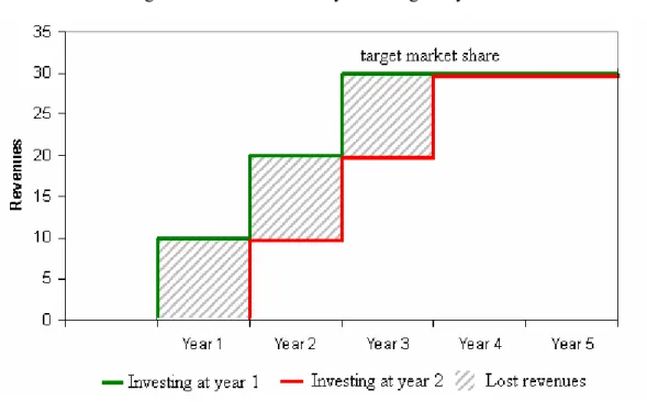
by the end of 2006. We assume that a one-year investment postponement causes revenues
to be lost for the following three years, although by a decreasing amount: hence the initial
delay does not lead to a parallel shift over time in the flow of revenues but the gap is filled
in a 3-year time horizon. Three years were in fact the expected time by a new entrant such
as Citéfibre in order to reach its target penetration. Three years also reflect the average time
invested one year earlier (see Figure 9). Thus the value assigned to the payout variable in
the Citéfibre case is obtained by multiplying by three the foregone revenues suffered in the
period in which the decision to postpone was made.
Per unit up-front costs are estimated by resorting to a study of the investment costs of
NGN published the French telecommunications regulator Arcep (2006): the average cost
estimated by Arcep (€500) has been decreased to take into account that in Paris the roll-out
of the fibre is less expensive due to the possibility of exploiting the sewage system. A
sanity check of this value has been carried out by comparing with the value inferred
directly using Citéfibre available data. The up-front cost is therefore assumed to be equal to
€400.
Figure 9 – Revenues lost by investing one year later
The annualized volatility of the log return has been estimated using bi-weekly stock
returns. Since Citéfibre was floated on Euronext on the 2nd December 2005, the sample size
is slightly above 45 observations. A higher frequency would have increased the accuracy of
the estimate by increasing the number of observations; however this might have entailed an
24
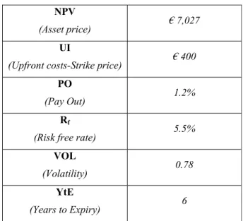
upward biased due to the very low liquidity of the stock. The Citéfibre input data are shown
in Table 1.
Table 1 – Citéfibre input data
NPV
(Asset price) € 7,027
UI
(Upfront costs-Strike price) € 400
PO
(Pay Out) 1.2%
Rf
(Risk free rate) 5.5%
VOL
(Volatility) 0.78
YtE
(Years to Expiry) 6
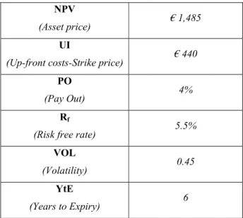
4.1.1.2 – Established telecommunication operator inputs
Parameters of an NGN investment by an established telecommunication operator differ
significantly from those applicable to a start-up firm. This is because all parameters and
outcomes have to be evaluated in incremental terms. For instance, the expected NPV of the
project is not equal to the overall project cash flow but it is computed as the incremental
revenues following the introduction of the new asset. The same logic applies to the
evaluation of the payout ratio and of up-front costs.
Also, in the case of the established operator, per unit up-front cost is based on the Arcep
study. The input value to the model takes into account that an established operator has to
incur some capital expenditures anyway (for instance, for the maintenance and upgrade of
traditional copper lines), even if it does not undertake the NGN investment.
The annual payouts (incremental revenues + cost savings) are computed as in the
Citéfibre example. The annual payout is thus equal to the difference between the NPV of
case of a 1-year postponement. The NPV is obtained by applying the perpetuity formula to
the annual net cash flow generated by the introduction of the new asset.
The net cash flows associated with an NGN project for an established operator do not
arise only from incremental revenues but also by cost savings. This clearly affects the
volatility of the NPV, since cost savings are reasonably steady and predictable. We have
assumed that in the case of an established operator half of the net cash flows derive from
incremental revenues: the VOL variable for an established operator is thus set equal to half
of that of Citéfibre25. Table 2 shows established telecommunication operator input data.
Table 2 – Established telecommunication operator inputs data
NPV
(Asset price) € 1,485
UI
(Up-front costs-Strike price) € 440
PO
(Pay Out) 4%
Rf
(Risk free rate) 5.5%
VOL
(Volatility) 0.45
YtE
(Years to Expiry) 6
25
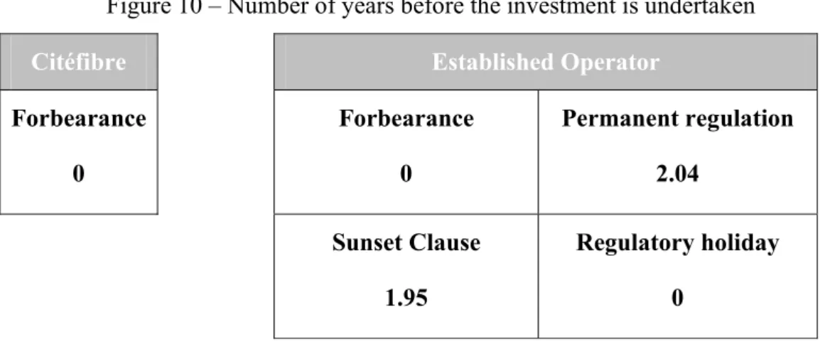
4.2 – Model outcome and the role of regulation
As already said, we follow the Cox et al. (1979)model to investigate the impact of
different regulatory regimes onto NGN investment decisions. Its outcomes include
expected optimal investment timing and optimal investment policy (i.e. critical values)26.
Since the timing of the investment is of particular interest to policy makers and to national
sectors regulators, we will focus on the interval between when the investment opportunity
arises and when the investment is expected to be undertaken, named fugit. The central
results of the simulations for the input data shown in Tables 1 and 2 are represented in
Figure 10.
Figure 10 – Number of years before the investment is undertaken
Citéfibre Established Operator
Forbearance
0
Forbearance
0
Permanent regulation
2.04
Sunset Clause
1.95
Regulatory holiday
0
For the sake of simplicity we divide the project lifespan into three phases. The first
phase includes the first six years of the project lifespan, which we define as the “volatile”
phase. The second phase (the “steady” phase) embraces years from the seven to the twelve,
while the third phase (the “terminal” one) includes the remaining years of the project
lifespan (from the thirteen to infinity). Differently from the steady and the terminal phases,
to refrain from the irreversible decision entails an insurance value in the volatile one.
26 Critical values can be used to determine the optimal subsidy i.e. the artificial increase of the NPV (either in
The parameters used for Citéfibre reflect the assumption that the new entrant operates
in absence of any regulation. By calibrating the model with the parameters of the new
entrant operator (see Table 3), we obtain a fugit variable equal to 0 (highlighted cell). The
model correctly predicts that the optimal policy for Citéfibre in the second half of 2005 was
to undertake the investment (which it did).
The volatility of returns on the investment carried out by the Parisian FttH operator is
such that any reduction of cash flows during the “volatile phase” (top row; left column) or
of cash flows in the “steady phase” (middle row; left column) tilts the decision to invest.
Thus, all regulatory interventions on the new entrant would prevent it from investing. The
outcome and a sensitivity analysis for a new entrant operator are presented in Table 3.
The sensitivity analysis concerns the up-front cost of the investment (strike price),
which is allowed to vary by ±12% with respect to the base value; the payout rate, whose
interval is assumed to lie in between ±0.5 around the central value of 1.2%; the volatility,
which we allow to be lower than the reported value of 0.78, if the stock were more liquid;
the NPV (asset price) of the project which can vary by ±20%. In most cases, the optimal
time to invest remains “now”. As expected, the investment tends to be deferred (up to
almost four years) when the investment cost rises or its payout falls; on the other hand, as
the NPV decreases, the project is delayed because the probability of not recovering the
Table 3 – Citéfibre outcomes data
Volatility
0.623 0.700 0.777
Up-front cost
Payout rate
NPV
5622 7027 8432 5622 7027 8432 5622 7027 8432
0.007 2.04 0.00 0.00 2.27 1.88 0.00 3.36 2.33 1.96
0.012 0.00 0.00 0.00 0.00 0.00 0.00 1.99 0.00 0.00
352
0.017 0.00 0.00 0.00 0.00 0.00 0.00 0.00 0.00 0.00
0.007 2.16 1.76 0.00 3.24 2.15 1.51 3.68 2.39 2.25
0.012 0.00 0.00 0.00 1.52 0.00 0.00 2.27 0.00 0.00
400
0.017 0.00 0.00 0.00 0.00 0.00 0.00 0.00 0.00 0.00
0.007 3.09 2.05 0.00 3.55 2.27 2.05 3.78 3.37 2.36
0.012 0.00 0.00 0.00 2.15 0.00 0.00 2.38 2.16 0.00
448
0.017 0.00 0.00 0.00 0.00 0.00 0.00 2.00 0.00 0.00
We can now turn to the case of the established operator. While in the case of the new
entrant we assumed absence of any regulation, with the established operator we are
interested at looking at the impact of different regulations on the timing of investment. We
consider four different regulatory scenarios: 1) Forbearance (absence of regulation); 2)
Permanent regulation; 3) Sunset clause; 4) Regulatory holiday. The intervention by the
regulator consists of a decrease in the annual net cash flow of the established operator by
27.5%. This reduction corresponds to a halving of the cost savings and the extra profits of
NGNs.
Initially we assume that the established operator is the only one which is evaluating
whether to invest in NGNs: the competitive situation is such that no alternative operator is
looking at building a next generation infrastructure. Therefore the incumbent has not to
rush (or delay) the investment in order to compete with infrastructure-based new entrants
(or to exploit somebody else’s network). In practice, with limited exceptions such as
Fastweb in Italy and Free in France, so far only incumbents have announced wide-ranging
other hand, by neglecting the competitive interplay between established operators and
competitors, a relevant factor in deciding the optimal timing of investment in NGNs might
be missed.
Regulatory forbearance. The regulatory forbearance consists of withdrawing
sector-specific ex ante regulation on next generation networks, i.e. mandated access to the
infrastructures and setting of the price at which access is imposed27. In the regulatory
forbearance, the authority leaves returns uncapped in both the volatile and the steady phase.
The forbearance scenario is modelled by assigning to the NPV and PO their initial values
i.e. those included in Table 2.
Results (see Figure 10 for a summary and Table 4 for the whole set) are obtained by
setting the up-front investment equal to €440 and the volatility equal to 0.45: they are
shown in the highlighted 3x3 matrix of Table 4. In the forbearance scenario (bottom row;
right column), which corresponds to the highest payout rate and NPV, investment is
undertaken immediately.
Sensitivity analysis is conducted on the investment up-front cost (±14%) and on
volatility. In all cases, except when the up-front investment cost and volatility take both
their highest values, in which case fugit is equal to two years, forbearance leads to
immediate investment.
From the point of view of our model, the regulatory forbearance is the most effective
solution in order to enhance investments. In fact the company decision to invest is based on
expectations of unconstrained net cash flows (both NPV and payout are unconstrained).
Clearly, our framework is inadequate to examine the competition issues raised by the
regulatory forbearance, which are causing so much concern with the European Commission
and regulators everywhere in Europe. In fact our model is only concerned with the amount
and the timing of investments: hence a regulatory forbearance is a first best solution almost
by construction.
27
In order to take care of the concerns by the EC, we should have introduced a different
objective function, based on the consumers’ welfare (or possibly the total welfare), to be
maximised. There are basically two ways to do so. One is to introduce the amount of
investment directly in the welfare function, as in Brandão and Sarmento (2007) and Kalmus
and Wiethaus (2006): the argument is that investment increases the quality of service,
hence benefits consumers directly. In the case of next generation networks, it can be argued
that new fibre infrastructures will indeed reduce the number of technical faults in the
network. However, in this case, the model would not include an obvious trade-off between
the degree of competition and the amount of investment. The second possibility is to
incorporate in the model the notion that, if forbearance leads to less competition in the
marketplace and therefore to an exit of alternative operators, then the established operator
which builds the NGNs may have to forego some extra revenues at the wholesale level.
These extensions are left for future work.
Permanent regulation. This measure is at the opposite extreme of the regulatory
spectrum than forbearance. The idea is that incumbent operators are forced by the regulator
to supply a wholesale service (bit-stream) based on NGN on request to alternative
operators. This option has been entertained by several European regulators, including the
Italian one. European established operators have usually retorted that the sale of wholesale
services based on NGN should take place under commercial freedom. Of course, one
crucial issue is the price of the wholesale service: Ofcom for instance has mentioned the
possibility to adjust the reference price of the NGN bit-stream in order to take into account
the risk of the investment.
In a permanent regulation scenario, national regulatory authorities cap returns both in the
volatile and in the steady phase. Permanent regulation is modelled by a 27.5% reduction of
PO, whose rate now becomes equal to 4%, and by a reduction of the NPV equivalent to a
27.5% of the cash flow over a period extended to 12 years, which is now equal to €1,291.
The lost payout, the expected NPV at the initial date and the NPV at expiry are all
reduced as a consequence: it becomes more convenient not to exercise the option than in
(middle row, left column) implies in fact an expected postponement of the investment of
about two years28. Sensitivity analysis suggests that the delay increases with the strike price
and the volatility, up to 3.48 years when both parameters take their maximum values in the
exercise.
Sunset clause. Sunset clauses are a regulatory tool which is more widespread in the US
than in Europe. Still, it could help to overcome some of the regulatory concerns raised by
the deployment of NGNs. The measure is that established operators which build new
networks are compelled to provide a wholesale permanent regulation bit-stream service
based on NGN, such as the one we discussed in the previous case, for a pre-determined
period of time. The rationale is that established operators can allegedly exploit the
advantage of having a larger market share to start with: hence, in principle, they need less
time to recoup the massive investment costs of NGNs. With a sunset close obligation,
alternative operators can make use of the established operator’s infrastructures, while they
build their own customer base and overcome the initial competitive disadvantage. After a
pre-defined number of years, the established operator is no longer obliged to rent the NGN
infrastructures at a cost and the alternative operators may either rent at commercial
conditions or build their own networks. The main rationale of the sunset clause is that it
creates the proper incentives for alternative operators to build their own infrastructures,
while at the same time reducing only partially the incentive for the established operator to
construct its own network.
The sunset clause scenario corresponds to a regulatory policy which intervenes in the
volatile phase, while it leaves returns uncapped in the steady phase of the project. In terms
of our model, the sunset clause scenario is modelled by subtracting to the initial value of
the NPV the 27.5 % of the net cash flow realised over a six year period (NPV is thus equal
to €1,388) and by reducing the initial PO by 27.5%, down to 4%. The sunset clause (middle
row centre column) results in a expected investment postponement of almost two years
(1.95).
28
Albeit the sunset clause can be preferred on theoretical grounds, our simulation suggests
that investment in NGNs ends up being postponed by almost the same amount of time as in
the permanent regulation case. This is because it affects the investment return during the
period – the first six years - in which it matters most for the purpose of the investment
decision, as uncertainty is still high and it makes sense to wait before undertaking the
project.
The sensitivity analysis shows that the waiting time is typically either zero or around
two years. Only when volatility and the up-front cost take the highest values, then the
postponement overcomes three years. In all instances the waiting time in the susnset clause
is slightly lower than the corresponding time under permanent regulation.
Regulatory holiday. This is another intermediate solution between the regulatory
forbearance and the permanent regulation. The regulator should impose no regulatory
obligations on the investments implemented in the initial period of the project up to the
expiry date. The rationale is that, in a real option framework, it is the uncertainty on the
distribution of future cash flows, hence of the net present values, which causes the company
to put off the project. As we saw, such uncertainty is very high at the beginning, when the
value of the reversibility (or protection) component is at its zenith. Uncertainty, hence the
insurance element, tends to become smaller in the following periods. If the aim of the
regulator is to create an environment conducive to investments, then it may decide to scrap
all regulatory obligations until uncertainty becomes sufficiently small. After that date, the
regulator can impose obligations with an impact on cash flows.
The benefit of a multiphase regulation policy that adjusts its tightness to the expected
decrease of the risk over time is twofold: it would act as an effective incentive where it is
needed (i.e. when the protection value against downside potential would refrain
telecommunication operators from investing); when the circumstances will be such as to
justify fibre deployment irrespectively of the regulatory context, the major benefit of the
investment could be directly transferred to consumers through the promotion of a fiercer
service based competition at retail level.
The proposed regulatory policy differs substantially from the regulatory holiday called
for by Deutsche Telekom29 for two main reasons: 1) it does not require a removal of all
forms of regulation (access, non discrimination, transparency obligation may indeed be
preserved) but it simply envisages a more favourable rate of return on investments
undertaken in the volatile phase; 2) the timeframe of the lenient regulatory phase is to be set
according to the reduction in the volatility rather than being based on the operator actual
investment plan: if the established operator does not launch its service within a certain date,
the more favourable regulatory conditions will be foregone30.
The regulatory holiday scenario is modelled by subtracting to the NPV initial value
27.5% of the net cash flow realised over a six year period (down to €1,388)31, whereas the
value of the payout rate is left as in the forbearance case (5.5%). The regulatory holiday
scenario (bottom row; middle column) results in immediate investment, as in the
forbearance case. This can be explained by the fact that the regulatory intervention applies
only to the period when uncertainty on the project returns is gone: hence, it does not affect
the decision on whether to undertake the project.
If we vary the values of the parameters, the fugit time remains basically unaffected and
equal to zero. Only when the up-front cost increases, then the investment is delayed by
around two years also in the regulatory holiday scenario.
In all scenarios the terminal phase of the project is assumed to be fully competitive and
thus out of the scope of regulation32.
29
In Germany, it was intruduced through a specific amendment to the German Law of Telecommunications. Such legal prevision has been fiercely opposed by the European Commission on the ground that the established operators would be able to limit the availability of access of new entrants, undermining competition in the market place. On this issue he EC has started an infringement procedure against Germany.
30
The regulatory holiday invoked by Deusche Telecom would be effective from the date of deployment.
31
The impact of regulation on NPV is measured as a percentage reduction of the cash flows accrued in the period regulation operates. Due to discounting the absolute value of foregone cash flows in a sunset clause scenario would be higher than absolute value of foregone cash flows due to a sunset clause policy. However since the aim of the model is to compare how the two alternative regulatory regimes perform in terms of incentives to invest with respect to their different time scopes we decided to neglect the discounting effect. This is done by applying the same NPV reduction both under the regulatory holiday scenario and the sunset clause scenario.
32 Note that in the sunset clause and in the regulatory holiday regimes, the length of the volatile and that of the