Stock market liquidity impact on economic development

(1)

Dissertação

Mestrado em Finanças Empresariais

Stock Market Liquidity Impact on Economic

Development

Tiago Miguel Santos Silva

(2)

i

Dissertação

Mestrado em Finanças Empresariais

Stock Market Liquidity Impact on Economic

Development

Tiago Miguel Santos Silva

Dissertação de Mestrado realizada sob a orientação da Doutora Professora Lígia Febra, Professora da Escola Superior de Tecnologia e Gestão do Instituto Politécnico de Leiria e coorientação da Doutora Professora Eduarda Fernandes, Professora da Escola Superior de Tecnologia e Gestão do Instituto Politécnico de Leiria.

(3)

ii Esta página foi intencionalmente deixada em branco.

(4)

iii Esta página foi intencionalmente deixada em branco.

(5)

iv

Agradecimentos

Gostaria de agradecer em especial ao meu pai, irmã e namorada por todo o apoio e compreensão demonstrados durante o período de elaboração desta dissertação.

Gostaria ainda de agradecer também à minha orientadora Prof. Lígia Febra e coorientadora Prof. Maria Eduarda Fernandes por todo apoio e ajuda que prestaram ao longo do desenvolvimento deste projeto, pois sem ele, não teria sido possível a conclusão desta dissertação.

Queria também agradecer a todos os meus amigos que de uma forma ou de outra contribuiram tanto para o desenvolvimento desta dissertação bem como para os necessários e importantes momentos de lazer e descontração.

(6)

v Esta página foi intencionalmente deixada em branco.

(7)

vi

Resumo

Este trabalho analisa a relação entre a liquidez do mercado de capitais e o desenvolvimento económico dos países, que ultimamente tem sido alvo de interesse de vários investigadores por se considerar que a liquidez do mercado de capitais tem um impacto considerável no desenvolvimento económico de um país. No entanto, todos os estudos conhecidos utilizam apenas no crescimento económico como proxy para o desenvolvimento económico, em vez de se aplicar um índice composto por várias dimensões de forma a representar o verdadeiro desenvolvimento económico de um país.

Assim, o objetivo principal deste trabalho é contribuir para este ramo da literatura, utilizando o Índice de Desenvolvimento Humano como proxy para o desenvolvimento económico. A liquidez do mercado de capitais foi calculada com base na medida de iliquidez de Amihud (2002), que é atualmente uma das medidas mais fidedignas desta área.

O estudo foi realizado com base numa amostra ampla e diversificada, contando com 59 países. O período amostral compreende-se entre 1990 e 2015, sendo os dados de frequência anual. Primeiro foi testada a correlação entre a liquidez e o desenvolvimento económico de cada país utilizando o teste não-paramétrico de correlação de Spearman. De seguida foram aplicados os modelos de regressão pooled OLS e de efeitos fixos ou aleatórios, sendo posteriormente escolhido o modelo mais adequado através dos testes F, Breusch-Pagan e Hausman. Quando analisados individualmente, a maioria dos países apresenta uma correlação positiva entre a liquidez do mercado de capitais e o desenvolvimento económico, sendo consistente com a relação positiva estatisticamente significativa da amostra global apresentada pelos modelos regressivos. Dividida a amostra global pelo nível de desenvolvimento económico dos países e pelo período anterior e posterior à crise económica de 2008, verifica-se existir alterações estatisticamente significativas do impact da liquididez no desenvolvimento económico dos países. Somente os países em desenvolvimento apresentaram uma relação negativa estatisticamente significativa entre as duas dimensões analisadas, contrariamente ao esperado. No entanto, este resultado poderá estar relacionado com as maiores dificuldades na transação de ativos, diminuindo a liquidez e desacelarando o crescimento económico.

Palavras-chave: Liquidez do mercado de capitais; desenvolvimento económico; Índice de Desenvolvimento Humano; Medida de iliquidez de Amihud (2002)

(8)

vii Esta página foi intencionalmente deixada em branco.

(9)

viii

Abstract

This work analyses the relationship between the stock market liquidity and the country’s economic development, which has been object of interest of many researches lately. The stock market liquidity is considered to have a huge impact on a country’s economic development. However, all the known studies focused on the economic growth as proxy for the economic development, instead of using a composition of various dimensions to explain the true economic development of a country.

Therefore, the main aim of this work is to contribute to this branch of the literature by using the Human Development Index as proxy for the economic development. The stock market liquidity was calculated based on the Amihud's (2002) illiquidity measure, which is one of the most reliable measures of this area.

This study was carried out based on a wide and diversified sample with 59 countries. The sample period is comprised between 1990 and 2015, with annual frequency data. Firstly, the correlations between the stock market liquidity and economic development are calculated for each country using the Spearman's non-parametric correlation test. Then, were applied the pooled OLS and fixed and random effects regression models, being the most suitable model then chosen through the F, Breusch-Pagan and Hausman tests. When analysed individually, most of the countries have a positive correlation coefficient between the stock market liquidity and economic development, which is consistent with the statistically significant positive relationship when analysing the global sample. Dividing the original sample by the level of economic development of the countries and by the period before and after the economic crisis of 2008, there are statistically significant changes in the impact of the stock market liquidity on the countries’ economic development. Only the developing countries presented a statistically significant negative relationship between the two analysed dimensions, contrary to the initial expectations. Still, this result may be related to the greater difficulties in the transaction of assets, reducing liquidity and slowing down economic growth.

Keywords: Stock market liquidity; economic development; Human Development Index; Amihud's (2002) illiquidity measure

(10)

ix Esta página foi intencionalmente deixada em branco.

(11)

x

List of figures

Figure 1 – HDI resume (Human Development Reports, n.d.) ... 6

Figure 2 – HDI coefficients against liquidity logarithm – developed countries ... 34

Figure 3 – HDI coefficients against liquidity logarithm – developing countries ... 35

Figure 4 - HDI coefficients against liquidity logarithm – pre-crisis era ... 35

Figure 5 - HDI coefficients against liquidity logarithm – post-crisis era ... 36

Figure 6 – Pooled OLS regression results – entire sample ... 52

Figure 7 – Fixed effects regression results – entire sample ... 53

Figure 8 – Random effects regression results – entire sample ... 54

Figure 9 – Pooled OLS regression results – economic development analysis ... 55

Figure 10 - Fixed effects regression results – economic development analysis ... 56

Figure 11 - Random effects regression results – economic development analysis .... 57

Figure 12 – Pooled OLS regression results – 2008 crisis analysis ... 58

Figure 13 - Fixed effects regression results – 2008 crisis analysis ... 59

(12)

xi Esta página foi intencionalmente deixada em branco.

(13)

xii

List of tables

Table 1 - Literature review resume (conclusive results) ... 14

Table 2 - Literature review resume (non-conclusive results)... 18

Table 3 – Sample by economic development level ... 25

Table 4 – Descriptive statistics resume for all sample ... 25

Table 5 – Descriptive statistics resume for the 38 developed countries ... 27

Table 6 – Descriptive statistics resume for the 21 developing countries ... 27

Table 7 – Descriptive statistics resume for all sampled countries – period 1990-2007 ... 28

Table 8 – Descriptive statistics resume for all sampled countries – period 2008-2015 ... 29

Table 9 – Spearman correlation values between HDI and liquidity for each country – positively correlated ... 31

Table 10 – Spearman correlation values between HDI and liquidity for each country – negatively correlated... 32

Table 11 - Spearman correlation values between HDI and liquidity for each country – not statistically correlated ... 32

Table 12 – Spearman correlation values between HDI and liquidity by sample ... 33

Table 13 – Fixed effects regression results – entire sample... 37

Table 14 – Fixed effects regression results – economic development analysis ... 38

Table 15 – Fixed effects regression results – 2008 crisis analysis ... 40

Table 16 – Descriptive statistics resume for all sample (resized data) ... 50

Table 17 – Descriptive statistics resume for the 38 developed countries (resized data) ... 50

Table 18 – Descriptive statistics resume for the 21 developing countries (resized data) ... 51

Table 19 – Descriptive statistics resume for all sampled countries – period 1990-2007 (resized data)... 51

Table 20 – Descriptive statistics resume for all sampled countries – period 2008-2015 (resized data)... 52

(14)

xiii Esta página foi intencionalmente deixada em branco.

(15)

xiv

List of symbols and abbreviations

HDI Human Development Index

GDP Gross Domestic Product

GNP Gross National Product

UN United Nations

GNI Gross National Income

HDRO Human Development Report Office

UNDP United Nations Development Programme

EU European Union

ASEAN Association of South-East Asian Nations

G20 Group of 20

USA United States of America

IV Instrumental Variables

VAR Vector Autoregressive

OLS Ordinary Least Square

ECM Error Correction Model

ARDL Autoregressive Distributed Lag

REM Random Effect Model

FEM Fixed Effect Model

(16)

xv Esta página foi intencionalmente deixada em branco.

(17)

xvi

1. Introduction

The relationship between the stock market development and the country’s economic development has been object of interest of many researchers. Hence, several models composed by various financial and economic variables have been developed to explain the relationship between these two elements. One of the most studied dimensions or proxy of the stock market development on these prediction models is the stock market liquidity, as it is considered to have a huge impact on the stock market development, which in turn is expected to have a positive impact on the economic development of a country.

The relationship between the stock market liquidity and the economic growth was studied by many authors throughout the years, as Levine(1991), Levine & Zervos (1998) and more recently by Rahman & Salahuddin (2010), Meichle, Ranaldo, & Zanetti (2011), Næs, Skjeltorp, & Ødegaard (2011), Florackis, Giorgioni, Kostakis, & Milas (2014), Smimou (2014), Apergis, Artikis, & Kyriazis (2015) e Galariotis & Giouvris (2015), to name a few. However, they all focus on economic growth and not on economic development as a composition of various dimensions like composite indices.

The economic development concept includes but it is not only the economic status of a country. Apart from that, it also takes into account the level of education and the health conditions of its population, for example. Thus, one should not use just a singular variable to capture the economic development but a composite index that includes social dimensions that are part of a country’s development.

The most commonly used variables to measure economic development are based on economic measures like Gross Domestic Product (GDP), unemployment rate, productivity, consumption and so on. Therefore, those works were in fact only capturing the economical dimension of a country’s development, which is only one part of its economic development. The main aim of this work is, therefore, to contribute to this branch of the literature by analysing the relationship between the stock market liquidity and the economic development by using the Human Development Index (HDI) as proxy for the economic development.

To our best knowledge, there is no study presenting a similar reasoning in terms of the choice of the economic development measurement, thus, this study presents new and significant conclusions about the stock market liquidity impact on the countries’ economic development, based on a wide and diversified sample containing 59 countries for the period

(20)

2 1990-2015, which enhances its representativeness. With these, more proactive politics or actions can be adopted by politicians or regulatory entities to stimulate the economic development through the stock market liquidity enhancement.

After this brief introduction the present dissertation is organized as follows. Next chapter presents a literature review, where is presented an overview about the economic development, stock market liquidity and later, an analysis of various papers that studied the relationship between the economic growth and the stock market development. The following chapter presents the methodology applied in this work, namely the sample composition, the chosen variables and the used empirical model. The results are presented on chapter 4 and finally, main conclusions are presented at the end of this dissertation, in the last chapter.

(21)

3

2. Literature review

To understand how economic development and stock market liquidity are linked, a small introduction to each theme is presented below: firstly, the economic development and then the stock market liquidity. Finally, this chapter concludes with several papers that analyse the relationship between the two.

2.1. Economic development

One of the first authors to define and explain economic development was Schumpeter in 1911 in his book “The Theory of Economic Development”. Schumpeter identified several factors as being able of influencing economic development, although classifying some of them as secondary like the wars, politic rebellion and cultural or spiritual issues phenomena. In his work, he affirmed that the main contributor to the economic development is the entrepreneur, as its actions are the main instrument to the economic development process and its disturbance. Entrepreneurs have the power of initiating innovative actions and to influence and change consumers’ preferences and needs, evolving this way the economic system. To Schumpeter, the entrepreneur does not save money or assets to start producing, instead, he uses capital supplied by the credit mechanisms of bankers or capitalists, which are therefore extremely important to enhance economic development. The discoveries and innovations promoted by the entrepreneurs generate new investment opportunities, creating employment and consequently, promoting growth (Croitoru, 2012; Śledzik, 2015).

Focusing on the underdeveloped economies, Hirschman wrote the “The Strategy of Economic Development” in 1958, aiming to help economists and governments to foster growth of those economies. He states that the less developed economies have limited growth initially due to the lack of ability to invest and in a later phase due to the scarce savings availability. The inability to perceive and carry out investment decisions or to overcome institutional obstacles impedes these economies from developing. To Hirschman, due to the scarce entrepreneurial ability, priorities must be defined in favour of interrelated industrial sectors which, as being related to each other, will enhance consequently the growth of other industries or sectors (Chenery, 1959).

(22)

4 The initial concept of development was therefore perceived as the necessity of increasing a countries’ total output along the time. However, some developed countries, in the 1950s and 1960s, realized that the standard of living of their population did not change even though the economic growth goals were being achieved. Governors realized that the increase of the country’s output did not radiate mass poverty, illiteracy or diseases. Hence, many economists removed the country’s output from the core of the economic development definition to include the focus on the eradication of poverty, illiteracy and diseases and on the enhance of the per capita output growth (Jahangir, 2011).

Economic development is not solely related to economic growth, but also to the improvement in human (or social) development (Birdsall, 1993). Another definition for economic development was proposed by Sen (2001) as he relates the development with people’s freedom. He stated that creating freedom for people and removing obstacles to greater freedom is the way to create development. The obstacles to freedom/development could be poverty, corruption, poor governance, lack of economic opportunities, lack of education or lack of health. Hence, the real development is only achieved by creating overlapping mechanisms that can promote the various freedom dimensions. Adelman (2001) affirms that the economic development combines sustainable growth, technological development, structural changes in production patterns and also social, political and institutional upgrading and improvements in human conditions.

Consequently, economic development is nowadays defined as multivariate concept, difficult to be defined in a single satisfactory sentence or to be measured in one single indicator (Jahangir, 2011).

The economic indicators per capita income (GDP per capita) growth was one of the firsts to be used to measure economic development, gaining popularity throughout the time. Due to this and to its easy availability, per capita income is the key indicator to measure the country’s economic performance. Using exclusively the GDP per capita growth to explain the economic development of a country has its advantages and disadvantages. It can show in a more comprehensive way if the economy is improving or not, being considered as a proxy for all the economic activity. However, GDP per capita does not consider many economic activities that do not involve money transactions although they have a real impact on the country’s economic development. The real nature of those activities or actions is also not considered in this measure, which could be useful of harmful to the society. As this is a quantitative and objective measure, it cannot express the impact of qualitative and subjective

(23)

5 elements like the level of happiness, justice, security, well-being, leisure of freedom of the people. As stated before, the economic development does not only comprehend the economic strand of a country but also the social and political strands. Therefore, to get an overview of the economic development of a country, one should use other social indicators like the literacy level, educational enrolment ratios, life expectancy, maternal or infant mortality rates or the access levels to drinking water and sanitation. Poverty or inequality levels can also be used to describe the social development (Jahangir, 2011).

To minimise the problems of using individual indicators and the risk of not seizing the real development level of a country, is possible to combine a selection of indicators to create a development index. The most popular is the Human Development Index, created by the United Nations (UN).

The main aim of HDI is to highlight that people and their capabilities should be the final criteria to assess the country development, not just economic indicators by themselves. With HDI is possible to understand how two countries with similar income per capita can have different human development results (Human Development Reports, n.d.).

HDI is a resume of three main dimensions of human development: a long and healthy life, having a decent living standard and being knowledgeable. It is a geometric mean of normalized indices for each of the mentioned dimensions (Human Development Reports, n.d.).

The health indicator used is the life expectancy at birth, the educational indicators are the mean of years of schooling for adults with 25 or more years and the expected schooling years for children with school entering age. To measure the standard of living is used the economic indicator Gross National Income (GNI) per capita. Then, the three scores are aggregated into a single index, using a simple geometrical mean (Human Development Reports, n.d.).

Although HDI is a composite index, it does not capture all the human development dimensions, as it does not reflect the effects of inequalities, poverty, security, empowerment, and so on. For those special cases, Human Development Report Office (HDRO) presents other composite indices more focused on inequality, gender disparity and poverty. The HDRO therefore recommends the use and analysis of other human development indicators and information to get a full picture of a country’s level of development (Human Development Reports, n.d.).

(24)

6 Figure 1 presents a resume of the HDI content and calculation.

Figure 1 – HDI resume (Human Development Reports, n.d.)

The HDI values for each country since 1990 are available and free on the United Nations Development Programme (UNDP) website, although not all countries have HDI values since that date because of data unavailability.

2.2. Stock market liquidity

The stock market liquidity is related to the volume of transactions, frequency of trading and the price impact (Datar, 2000). In other words, liquidity describes the ease of buying or selling an asset or security without any major fluctuation on price. For example, if a stock has a high trading volume that is not dominated by selling, the bid price and the ask price will be close to each other. Thus, when bid and ask spread gets higher, the stock becomes more illiquid. To simplify, from now on, stock market liquidity will be referred only as liquidity.

Relative spread is the difference between ask and bid prices and it reflects the cost of immediacy. It measures the implicit cost of trading shares and it is calculated as the quoted spread (the difference between the best bid and ask prices) as a fraction of the midpoint price (the average of the best bid and ask prices).

, , 1 , , , ( ) ( ) / 2 ASK BID T i t i t ASK BID t i t i t i T T p p p p RS D = − + =



(2.1)

Where DT is the number of observations (or observed days), pi,tASK and pi,tBID is respectively the ask and bid price at day t for stock i. Overall, relative spread is an illiquidity

(25)

7 measure, as the higher the value, the more illiquid the stock due to large implicit costs of trading.

Lesmond, Ogden, & Trzcinka (1999) developed a measure of the transaction costs, based on daily returns, thus, independent from the quotations or the order book. The authors use the frequency of zero returns to determine an implicit cost of trading required for a stock’s price not to move while the market return changes. To explain this measure nature, they use the market model (2.2).

it i i mt it

R = +a b R +  _(2.2)

Where Rit is the return of security i on time t, Rm is the market’s return at time t, a and

b are respectively a constant term and a regression coefficient and ε an error term. If the

market return changes, the security’s return should also change according to the above equation. But if it does not, it may indicate that the trading cost might be higher than the price movement that should have occurred. To identify this “zero return” moments, the authors define cost bands around the stock price and consider that the wider the cost band, more illiquid is the security.

In 1984, Roll published an estimate of the implicit spread called effective bid-ask spread. This measure differs from the standard bid-ask spread by using the serial covariance of successive price movements. The estimator is defined as present below.

ˆ cov

s= −S (2.3)

Where ŝ is assumed to be a constant effective spread and Scov is the first order serial covariance of successive returns.

For some markets, some microstructure data on transactions and quotes are not available for long time periods. To overcome this problem, Amihud (2002) developed an illiquidity measure that uses daily data on returns and volume of transactions, that is available for most of the markets over long time periods. The author computed the stock illiquidity as the average ratio of daily absolute return to the (dollar) trading volume on that day. 1 / Diy iyd iyd t iy iy R VOLD ILLIQ D = =



(2.4)

(26)

8 Where Diy is the number of days with data available for stock i in year y, Riyd is the return of stock i on day d of year y and VOLDivyd is the respective daily volume in dollars. The reason that it is called an illiquidity measure is that a high value indicates a high price impact of trades which leads to low liquidity. So, this ratio shows the price changes percentage in relation to the daily trading volume.

The following measures can be used to measure both the stock market liquidity as well as the stock liquidity. The turnover ratio and value of traded shares ratio are two of the most used liquidity measures, mainly due to its calculus simplicity. The first is calculated dividing the total value of the traded shares on the stock exchange by the total value of listed shares on the stock exchange. The second is defined by the ratio between the total value of traded shares on the stock exchange and the GDP.

Goyenko, Holden, & Trzcinka (2009) evaluated the performance of various liquidity measures, including the ones cited before, and concluded that the measures based on daily data deliver good estimations of high frequency transaction costs benchmarks. They also state that more recently, apart the Amihud's (2002) illiquidity measure and the Lesmond, Ogden, & Trzcinka (1999) estimator, the performance of all measures deteriorated.

2.3. Economic growth and liquidity

The majority of the authors are focused on how the stock market or banking development influences the economic growth, studying these areas together (Anyamele, 2010; Beck & Levine, 2004; Caporale, Howells, & Soliman, 2004; Næs et al., 2011; Pradhan, Arvin, Hall, & Bahmani, 2014; Wu, Hou, & Cheng, 2010; Zhu, Ash, & Pollin, 2004). Only a few, study the stock market development effect on the economic development in depth, using various measures for the same issue, trying to capture all the effects of a specific dimension (Apergis et al., 2015; Florackis et al., 2014; Levine & Zervos, 1998; Næs et al., 2011; Smimou, 2014). Stock market liquidity is one of the main dimensions used to define the stock market development. Many have studied the linkage between liquidity and the economic growth and its causality direction, i.e. which one influences the other: if it is liquidity that lead to economic growth, vice-versa or even if both can enhance each other (Carp, 2012; Enisan & Olufisayo, 2009; Galariotis & Giouvris, 2015; N’Zué, 2006; Næs et al., 2011; Nurudeen, 2009; Pradhan, Arvin, & Ghoshray, 2015; Pradhan et al., 2014;

(27)

9 Ramkelawon, Khan, & Sunecher, 2015; Rousseau & Wachtel, 2000; Smimou, 2014; Srinivasan, 2014).

Although there are so many authors trying to explain how these two dimensions are linked together (Carp, 2012; Enisan & Olufisayo, 2009; Galariotis & Giouvris, 2015; N’Zué, 2006; Næs et al., 2011; Nurudeen, 2009; Pradhan et al., 2015, 2014; Ramkelawon et al., 2015; Rousseau & Wachtel, 2000; Smimou, 2014; Srinivasan, 2014), there is no consensus about which liquidity measure and economic development variable reveal or characterise better the information contained in both dimensions and how they are linked. This tendency extends to the methodologies applied by the various authors, which lead to different conclusions about if stock market liquidity impacts on economic growth or vice-versa and about the impact of each other and its relevance. The countries included in the sample and the time span selected by the authors also vary considerably, which can be other reason for the results’ inconsistencies.

One of the first endogenous models about the relationship between the stock market and the economic growth was developed by Levine in 1991, that also encompassed the tax policy effect. The conclusions are that the stock market can promote growth by facilitating the ability of trading firms’ ownerships without disrupting its productivity and allowing investors to have a diverse portfolio. Thus, a liquid stock market can promote the investment on high return projects and hence stimulating earnings and productivity growth, by lowering the cost of capital.

Since Levine (1991) several other studies have been published on the topic, the majority of which state that there is a positive relationship between the economic development/growth and the stock market liquidity (Ahmad, Etudaiye-Muhtar, Matemilola, & Bany-Ariffin, 2016; Apergis et al., 2015; Beck & Levine, 2004; Caporale et al., 2004; Carp, 2012; Castillo-Ponce, Rodriguez-Espinosa, & Gaytan-Alfaro, 2015; Cooray, 2010; Enisan & Olufisayo, 2009; Florackis et al., 2014; Levine & Zervos, 1998; Meichle et al., 2011; Næs et al., 2011; Ngare, Nyamongo, & Misati, 2014; Nowbutsing & Odit, 2009; Pradhan et al., 2015, 2014; Rahman & Salahuddin, 2010; Rousseau & Wachtel, 2000; Smimou, 2014; Srinivasan, 2014; Wu et al., 2010). The time span analysed by these authors vary significantly, both in terms of starting and ending years - Næs et al. (2011) captured data since 1947 whereas Srinivasan (2014) analysed the data available until 2013 – as well as its length that diverge from 11 years (Cooray, 2010) to 61 years (Næs et al., 2011). However, most of them examine data of 20 to 30 years, mainly after 1975.

(28)

10 The composition and length of the sample differ a lot between the various studies. For example, the biggest samples have 47 countries (Levine & Zervos, 1998; Rousseau & Wachtel, 2000), followed by Beck & Levine (2004) and Cooray (2010) that analysed 40 and 35 countries, respectively. There are also some authors that studied only one country, for instance, Cote D’Ivoire by N’Zué (2006), Nigeria by Nurudeen (2009), Mauritius by Nowbutsing & Odit (2009), Pakistan by Rahman & Salahuddin (2010), Switzerland by Meichle et al. (2011), Romania by Carp (2012), India by Srinivasan (2014), United Kingdom by Florackis et al. (2014),Canada by Smimou (2014) or Mexico by Castillo-Ponce et al. (2015). Other studies focus on a specific group of countries, for example Ahmad et al. (2016), Enisan & Olufisayo (2009) and Ngare et al. (2014) that studied only African countries, Wu et al. (2010) that analysed 13 European Union (EU) countries, Pradhan et al. (2014) that studied the 26 countries of the Association of South-East Asian Nations (ASEAN) regional forum or Pradhan et al. (2015) with the 19 countries with biggest economies plus the EU (G20).

In terms of the variables used, to measure the economic development/growth, most of the authors tend to use the GDP in various forms – real or nominal, total or per capita, growth percentage, logarithm form or even dividing it by levels. Others use a derived form of it, together with other variables like capital stock growth, productivity growth and savings (Levine & Zervos, 1998) or the real consumption, real investment and unemployment rate (Apergis et al., 2015; Næs et al., 2011) or even with the industrial production and market returns (Smimou, 2014). Srinivasan (2014) used only the industrial production as proxy to study the impact of the stock market on the Indian’s economic development.

Relatively to the liquidity measures, approximately half of the authors use only one variable to characterize the stock market liquidity, whilst the other half test the relationship of two, three or even four variables. The most commonly used ones are the turnover ratio, value of shares traded ratio and Amihud's (2002) illiquidity measure. The first two were applied in both newer and older articles (for example in Ahmad et al. (2016), Apergis et al. (2015), Levine & Zervos (1998), Pradhan et al. (2015), Rousseau & Wachtel (2000) or Zhu et al. (2004)) while the later were only applied in newer studies (as it became more popular and due to its later appearance).

Lastly, many control variables were used in the analysed papers where each one applies mainly between three to seven different variables in its study. Meichle et al. (2011) even apply 36 variables in total (including the dependent variables which in some tests are

(29)

11 used as control variables). These are predominantly measures of other dimensions of the stock market - for example, capitalization, market returns, volatility, etc. - (Caporale et al., 2004; Enisan & Olufisayo, 2009; Galariotis & Giouvris, 2015; Levine & Zervos, 1998; Nowbutsing & Odit, 2009; Zhu et al., 2004), bank sector (Ahmad et al., 2016; Anyamele, 2010; Pradhan et al., 2014) or country’s economy - for example schooling enrolment, government expenditures, unemployment rate, private and public investment, etc. - (Hou & Cheng, 2017; Matadeen & Seetanah, 2015; Ngare et al., 2014; Rahman & Salahuddin, 2010; Ramkelawon et al., 2015; Smimou, 2014). It is also commonly used the lagged dependent variable (Adjasi & Biekpe, 2006; Apergis et al., 2015; Florackis et al., 2014; Ngare et al., 2014) or other measures of the economic development of the studied country or even other main economies, mainly the United States of America (USA) (Florackis et al., 2014; Smimou, 2014).

In terms of the chosen methodology, it seems that there is no consensus of which one is better to determine the relationship between the country’s economic development and the respective stock market. The most commonly used, but only applied in four articles each, were the Instrumental Variables (IV) (Apergis et al., 2015; Levine & Zervos, 1998; Næs et al., 2011; Smimou, 2014) and the Vector Autoregressive (VAR) models (Caporale et al., 2004; Carp, 2012; Pradhan et al., 2015; Rousseau & Wachtel, 2000). Many variations of least square regressions were also applied (Beck & Levine, 2004; Levine & Zervos, 1998; Ngare et al., 2014) and to analyse the causality between the variables, the majority of the authors gave preference to the Granger causality test (Carp, 2012; Enisan & Olufisayo, 2009; Næs et al., 2011; Nowbutsing & Odit, 2009; Pradhan et al., 2015, 2014; Rousseau & Wachtel, 2000; Smimou, 2014; Srinivasan, 2014).

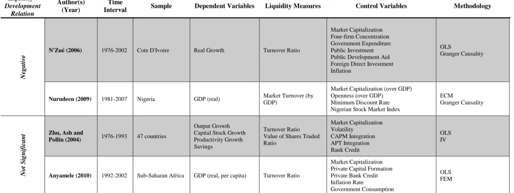
In terms of conclusions of these studies, as mentioned before, there is no consensus. N’Zué (2006) and Nurudeen (2009), for example, concluded that the stock market liquidity has a statistically significant negative impact on the country’s economic development. Studying, respectively, Cote D’Ivoire between 1976 to 2002 and Nigeria between 1981 to 2007, using similar dependent variables (the first used economic growth while the later the real GDP) and liquidity variables (N’Zué (2006) used the turnover ratio whereas Nurudeen (2009) applied the market turnover over GDP), both verified that exists a negative impact of the stock market liquidity on the economic growth. In terms of control variables, N’Zué (2006) focused more on measuring other dimensions of the government policy while Nurudeen (2009) used four other variables that measured the Nigerian stock market

(30)

12 development. The first used an Ordinary Least Square (OLS) model while the second an Error Correction Model (ECM), though, both applied the Granger causality test.

Contrarily to the previously mentioned authors, Zhu, Ash, & Pollin (2004) and Anyamele (2010) did not find any statistically significant relationship between the stock market liquidity and the chosen samples. Using OLS and IV methods, with the output, capital stock and productivity growth and savings as dependent variables, the turnover and value of traded shares ratios and other measures of stock market bank development as control variables, Zhu, Ash, & Pollin (2004) did not find any significant conclusion about this relationship. The same happened with Anyamele (2010) when applying the OLS method with real GDP per capita as the dependent variable, turnover ratio as liquidity measure and other measures of stock market, bank and economic development as control variables.

There are also some authors that got different conclusions when using different variables, methods, countries or sub-samples (divided by various conditions) (Adjasi & Biekpe, 2006; Cheng, 2012; Galariotis & Giouvris, 2015; Hou & Cheng, 2017; Matadeen & Seetanah, 2015; Ramkelawon et al., 2015). For example, using a sample composed by 14 African countries and the same methodology as Levine & Zervos (1998) during the period 1975-2001, Adjasi & Biekpe (2006) found that when the turnover ratio is used as liquidity measure, stock market liquidity does not play a significant role on the economic growth, whereas when using the value of traded shares ratio, it has a positive impact on it. Cheng (2012) found that in Taiwan, stock market liquidity had a positive impact on the economic growth before the financial openness in 1982. However, it turned negative afterwards, possibly due to the excess of liquidity caused by noise traders, which did not allow country’s economy to develop. The author applied a VAR model, during the period 1973-2007, with real GDP in logarithm form as the dependent variable, turnover ratio as liquidity measure and three other financial measures as control variables. Ramkelawon et al. (2015) and Matadeen & Seetanah (2015), when studying the Mauritius’s stock market liquidity during the years 1989-2011 and 1988-2011, respectively, using the GDP as the dependent variable and the liquidity measures turnover ratio and value of traded shares ratio, had different conclusions when applying different methodologies or different forecasts . The first, applying the Autoregressive Distributed Lag (ARDL) method found that the liquidity had a negative impact on the Mauritius GDP, whereas when applying an ECM, the impact turned out to be positive. The second, concluded that in the long run, the stock market liquidity would have a positive impact on the GDP, while in the short run it has no significance. In

(31)

13 2015, Galariotis & Giouvris studied the stock market liquidity of Canada, France, Germany, Italy, Japan, UK and USA by means of the use of an IV model during the period 1995-2013. Using the GDP, unemployment rate, personal consumption and private investment as dependent variables and the Amihud's (2002) illiquidity measure and the (Roll, 1984) spread to replicate the stock market liquidity (these were used separately), the authors got different results depending on the country that were studying and liquidity measure chosen. Lastly, Hou & Cheng (2017) applied an ECM on 31 countries during the period 1981-2008 and concluded that the relationships vary when dividing the sample by low and high GNI or by low and high financial development and for different forecasts. For example, the stock market liquidity has a positive impact on the low GNI group in the long run, whereas for the same forecast but with the high GNI sub sample this relationship is not significant.

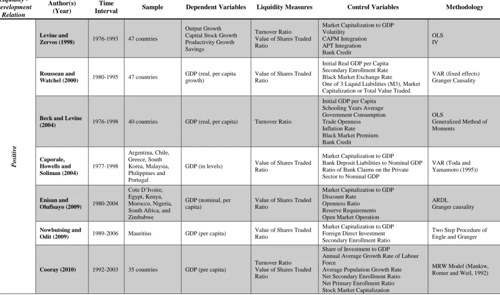
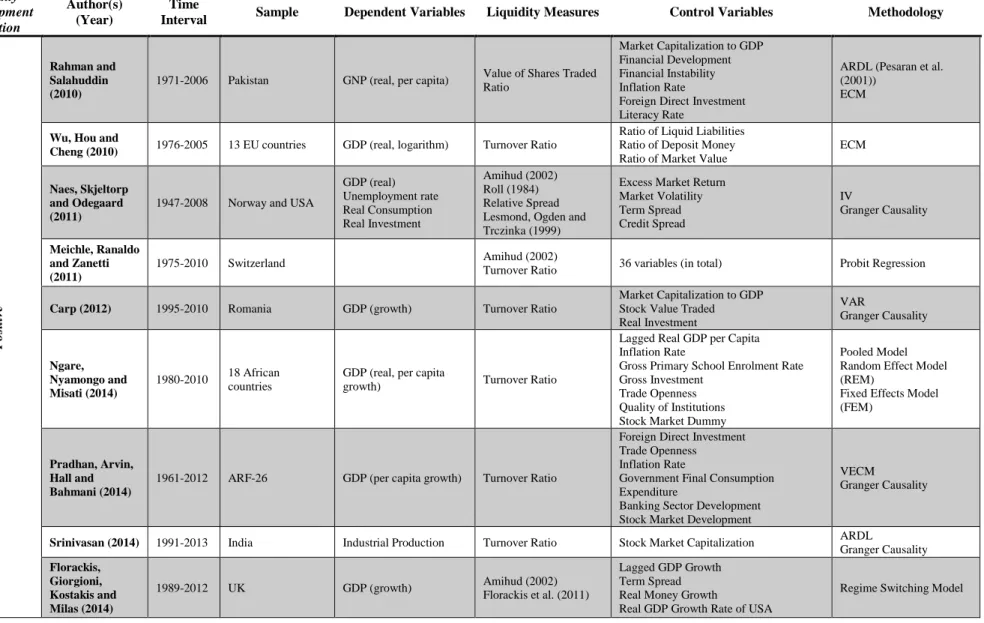
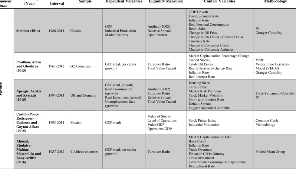
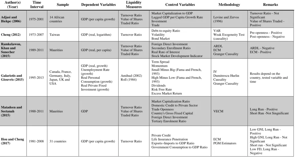
To resume all the literature review presented above, Table 1 and Table 2 present the main information about the mentioned articles.

(32)

14

Table 1 - Literature review resume (conclusive results)

Liquidity - Development Relation Author(s) (Year) Time

Interval Sample Dependent Variables Liquidity Measures Control Variables Methodology

Po siti ve Levine and Zervos (1998) 1976-1993 47 countries Output Growth Capital Stock Growth Productivity Growth Savings

Turnover Ratio Value of Shares Traded Ratio Market Capitalization to GDP Volatility CAPM Integration APT Integration Bank Credit OLS IV Rousseau and Watchel (2000) 1980-1995 47 countries

GDP (real, per capita growth)

Value of Shares Traded Ratio

Initial Real GDP per Capita Secondary Enrollment Rate Black Market Exchange Rate

One of 3:Liquid Liabilities (M3), Market Capitalization or Total Value Traded

VAR (fixed effects) Granger Causality

Beck and Levine

(2004) 1976-1998 40 countries GDP (real, per capita) Turnover Ratio

Initial GDP per Capita Schooling Years Average Government Consumption Trade Openness Inflation Rate Black Market Premium Bank Credit OLS Generalized Method of Moments Caporale, Howells and Soliman (2004) 1977-1998 Argentina, Chile, Greece, South Korea, Malaysia, Philippines and Portugal

GDP (in levels) Value of Shares Traded

Ratio

Market Capitalization to GDP

Bank Deposit Liabilities to Nominal GDP Ratio of Bank Claims on the Private Sector to Nominal GDP

VAR (Toda and Yamamoto (1995)) Enisan and Olufisayo (2009) 1980-2004 Cote D’Ivoire, Egypt, Kenya, Morocco, Nigeria, South Africa, and Zimbabwe

GDP (nominal, per capita)

Market Capitalization to GDP Discount Rate

Openness Ratio Reserve Requirements Open Market Operation

ARDL

Granger causality

Nowbutsing and

Odit (2009) 1989-2006 Mauritius GDP (per capita)

Market Capitalization to GDP Foreign Direct Investment Secondary Enrollment Ratio

Two Step Procedure of Engle and Granger

Cooray (2010) 1992-2003 35 countries GDP (per capita)

Turnover Ratio Value of Shares Traded Ratio

Share of Investment to GDP

Annual Average Growth Rate of Labour Force

Average Population Growth Rate Net Secondary Enrollment Ratio Net Primary Enrollment Ratio Stock Market Capitalization

MRW Model (Mankiw, Romer and Weil, 1992)

(33)

15

Table 1 - Literature review resume (conclusive results) (Cont.)

Po siti ve Rahman and Salahuddin (2010)

1971-2006 Pakistan GNP (real, per capita) Value of Shares Traded

Ratio

Market Capitalization to GDP Financial Development Financial Instability Inflation Rate

Foreign Direct Investment Literacy Rate

ARDL (Pesaran et al. (2001))

ECM

Wu, Hou and

Cheng (2010) 1976-2005 13 EU countries GDP (real, logarithm) Turnover Ratio

Ratio of Liquid Liabilities Ratio of Deposit Money Ratio of Market Value

ECM

Naes, Skjeltorp and Odegaard (2011)

1947-2008 Norway and USA

GDP (real) Unemployment rate Real Consumption Real Investment Amihud (2002) Roll (1984) Relative Spread Lesmond, Ogden and Trczinka (1999)

Excess Market Return Market Volatility Term Spread Credit Spread IV Granger Causality Meichle, Ranaldo and Zanetti (2011) 1975-2010 Switzerland Amihud (2002)

Turnover Ratio 36 variables (in total) Probit Regression

Carp (2012) 1995-2010 Romania GDP (growth) Turnover Ratio

Market Capitalization to GDP Stock Value Traded Real Investment VAR Granger Causality Ngare, Nyamongo and Misati (2014) 1980-2010 18 African countries

GDP (real, per capita

growth) Turnover Ratio

Lagged Real GDP per Capita Inflation Rate

Gross Primary School Enrolment Rate Gross Investment

Trade Openness Quality of Institutions Stock Market Dummy

Pooled Model Random Effect Model (REM)

Fixed Effects Model (FEM)

Pradhan, Arvin, Hall and Bahmani (2014)

1961-2012 ARF-26 GDP (per capita growth) Turnover Ratio

Foreign Direct Investment Trade Openness Inflation Rate

Government Final Consumption Expenditure

Banking Sector Development Stock Market Development

VECM

Granger Causality

Srinivasan (2014) 1991-2013 India Industrial Production Turnover Ratio Stock Market Capitalization ARDL

Granger Causality Florackis,

Giorgioni, Kostakis and Milas (2014)

1989-2012 UK GDP (growth) Amihud (2002) _{Florackis et al. (2011)}

Lagged GDP Growth Term Spread Real Money Growth

Real GDP Growth Rate of USA

(34)

16

Po siti ve Smimou (2014) 1986-2011 Canada GDP Industrial Production Market Returns Amihud (2002) Relative Spread Open Interest GDP Growth Unemployment Rate Inflation Rate

Real Personal Consumption Retail Sales

Change in Oil Price

Change in US Dollar - Canada Dollar Currency Rate

Change in Consumer Credit Change in Consumer Attitudes

IV

Granger Causality

Pradhan, Arvin and Ghoshray (2015)

1961-2012 G20 countries GDP (real, per capita

growth)

Turnover Ratio Total Value Traded

Market Capitalization Percentage Change Traded Stocks

Crude Oil Prices

Real Effective Exchange Rate Inflation Rate

Real Interest Rate

VAR

Vector Error Correction Model (VECM) Granger Causality Apergis, Artikis and Kyriazis (2015) 1994-2011 UK and Germany GDP (real, growth) Real Consumption (growth)

Real Investment (growth) Unemployment Rate (growth)

Amihud (2002) Turnover Ratio Relative Spread Total Value Traded

Housing Starts Term Spread Market Risk Premium Stock Market Volatility Short-term Interest Rate Default Spread

Lagged Dependent Variable

Toda-Yamamoto Causality IV Castillo-Ponce Rodriguez- Espinosa and Gaytan-Alfaro (2015) 1993-2011 Mexico GDP (real) Value of Stocks Level of Operations Value/GDP Operations/GDP

Stock Prices Index Industrial Production Common Cycle Methodology Ahmad, Etudaiye-Muhtar, Matemilola and Bany-Ariffin (2016)

1987-2012 9 African countries GDP (real, per capita

growth) Turnover Ratio

Market Capitalization to GDP Bank Credit

Inflation Rate Trade Openness Financial Crisis Dummy Gross Investment

Government Consumption Expenditure Real Interest Rate

(35)

17

Ne

g

a

ti

ve

N'Zué (2006) 1976-2002 Cote D'Ivoire Real Growth Turnover Ratio

Market Capitalization Four-firm Concentration Government Expenditure Public Investment Public Development Aid Foreign Direct Investment Inflation

OLS

Granger Causality

Nurudeen (2009) 1981-2007 Nigeria GDP (real) Market Turnover (by

GDP)

Market Capitalization (over GDP) Openness (over GDP)

Minimum Discount Rate Nigerian Stock Market Index

ECM Granger Causality No t S ig n ifi ca n

t Zhu, Ash and

Pollin (2004) 1976-1993 47 countries

Output Growth Capital Stock Growth Productivity Growth Savings

Turnover Ratio Value of Shares Traded Ratio Market Capitalization Volatility CAPM Integration APT Integration Bank Credit OLS IV

Anyamele (2010) 1992-2002 Sub-Saharan Africa GDP (real, per capita) Turnover Ratio

Market Capitalization Private Capital Formation Private Bank Credit Inflation Rate

Government Consumption

OLS FEM

(36)

18

Table 2 - Literature review resume (non-conclusive results)

Author(s) (Year)

Time

Interval Sample Dependent Variables

Liquidity

Measures Control Variables Methodology Remarks

Adjasi and

Biekpe (2006) 1975-2001

14 African

countries GDP (per capita growth)

Market Capitalization to GDP Lagged GDP per Capita Growth Rate Investment

Trade

Levine and Zervos (1996)

Turnover Ratio - Not Significant

Value of Shares Traded -Positive

Cheng (2012) 1973-2007 Taiwan GDP (real, logarithm) Turnover Ratio

Debt-to-equity Ratio Volatility

Bond Market

VAR

Weak Exogeneity Test (causality) Pre-openness - Positive Post-openness - Negative Ramkelawon, Khan and Sunecher (2015)

1989-2011 Mauritius GDP (real, per capita)

Foreign Direct Investment Secondary Enrollment Ratio Real Rate of Interest

Stock Market Development Indicator

ARDL ECM Granger Causality ARDL - Negative ECM - Positive Galariotis and Giouvris (2015) 1995-2013 Canada, France, Germany, Italy, Japan, UK and USA GDP (real, growth) Unemployment Rate (growth) Real Personal Consumption (growth) Real Private Fixed Investment (growth)

Amihud (2002) Roll (1984)

Term Spread Momentum

Small Minus Big (Fama and French, 1993)

High Minus Low (Fama and French, 1993)

Dividends Risk Free Rate Excess Market Return

IV

Dumitrescu Hurlin Causality Granger Causality

Results depend on the country, tested variable and time Matadeen and Seetanah (2015) 1988-2011 Mauritius GDP Turnover Ratio Value of Shares Traded Ratio

Market Capitalization Ratio Domestic Credit to Private Sector Trade Openness

Country's Gross Fixed Capital Foreign Direct Investment Tertiary Enrolment Ratio

VECM Long Run - Positive

Short Run -Not Singnificant

Hou and Cheng

(2017) 1981-2008 31 countries GDP (per capita growth) Turnover Ratio

Private Credit

Life Insurance Penetration Exports+Imports to GDP Ratio Government Consumption to GDP Ratio

ECM

PGM Estimators

Low GNI, Long Run - Positive

High GNI, Long Run - Not Significant

Short run - Not Significant Low FD, Long Run - Negative

(37)

19

3. Methodology

In this chapter research hypotheses are presented and justified, as well as the empirical model chosen to test them. It starts with the presentation of the three analysed hypotheses related with the relationship between economic development and stock market liquidity, followed by the empirical model presentation, its constituent variables and calculation formulas as well as the applied methodology. In the last sub-chapter, the sample is presented and analysed by means of its descriptive statistics.

3.1. Research hypotheses

As previously mentioned, the main aim of this study is to examine the relationship between the stock market liquidity and the countries’ economic development. Thus, the first hypothesis is the following:

H1: The stock market liquidity has a positive impact on the countries’ economic

development.

Following the reasoning of Schumpeter in 1911, the key factor for the development is a well-developed financing system. Being the stock market a financing system, its development is extremely important for the companies that use them to obtain credit. One of the most used stock market development indicators is the stock market liquidity, being positively associated with the development level. This assumption meets the initial beliefs of many similar studies like for instance Carp (2012), Galariotis & Giouvris (2015), Næs et al. (2011), Pradhan, Arvin, & Ghoshray (2015), Ramkelawon, Khan, & Sunecher (2015), Rousseau & Wachtel (2000) or Smimou (2014), although several other have reached different conclusions.

After this analysis, the original sample is divided in two different ways in order to comprehend if there is any difference between the relationship behaviour and if the initial beliefs are correct across all countries and/or set of countries. The first, similarly to the Adjasi & Biekpe (2006), and Hou & Cheng (2017) works, aims to examine if the stock market liquidity affects differently the countries’ economic development depending on the countries’ development classification, although these two studies present opposite conclusions. The second analysis is relatively to the 2008’s financial crisis impact and aim

(38)

20 to verify if the stock market liquidity impact on the economic development of its country is different before and after that crisis. After a crisis of this magnitude, is expected that the investors get more cautious due to the big losses that most of them suffered during the crisis. This leads to less and more pondered transactions, which therefore decrease the stock market liquidity. Resuming, the other two hypotheses tested are defined as follows:

H2: The relationship between the stock market liquidity and the economic development

is different between the developed countries and the developing countries;

H3: The relationship between the stock market liquidity and the economic development

is different before and after the great financial crisis of 2008.

3.2. Empirical model and research variables

As stated before, the main aim of this study is to evaluate the impact of the stock market liquidity on the country’s economic development, defining for that the HDI coefficient as the dependent variable and the logarithm of the inverse of the Amihud's (2002) illiquidity measure as the main independent variable, along with other control variables.

In order to check if the stock market liquidity is related with the country’s development level and to answer to the first research hypothesis stated above, one has to verify the non-parametric correlation between the main variables, namely the HDI coefficient and the stock market liquidity for each country. This correlation is evaluated by means of the Spearman’s correlation test. The Spearman’s correlation coefficient or Spearman’s rho is a nonparametric test to check if the two examined variables have a monotonic behaviour, this is, if the relationship can be described by a monotonic function. The results are between -1 and 1, where -1 indicates a perfect negative monotone correlation, 1 indicates a perfect positive monotone correlation and 0 no correlation at all. This test is done using IBM SPSS software. Besides studying the nature of the correlation between the two variables, a significance test will be applied to check if the hypothetic correlations are statistically significant or not, this is, if they are reliable or not.

Additionally, and following the reasoning of the base models presented namely by Ahmad et al. (2016), Apergis et al. (2015), Florackis et al. (2014) or Galariotis & Giouvris (2015), the empirical model developed to analyse the relationship between a country’s the economic development and the stock market liquidity is given as follows:

(39)

21

, 1 , 1 2 , 1 3 , 1 4 , 1 5 , 1 ,

i t i t i t i t i t i t i t

HDI = +

 

LIQ − +



MC − +



GDP − +



MYS − +



LE − +



(3.1) Where HDIi,t is the HDI value of the current year of the country i, β1, …, β5 are the estimation coefficients for each variable, LIQi,t-1 is the stock market liquidity value of the country i of the previous year, MCi,t-1 is the market capitalization over the GDP of the country

i of the previous year, GDPi,t-1 is the logarithm of real GDP per capita of country i of the previous year, MYSi,t-1 is the mean years of schooling logarithm of the country i of the previous year and LEi,t-1 is the life expectancy at birth logarithm of the country i of the previous year. Finally, εi,t is the regression error term.

The dependent variable (HDIi,t) is applied directly in the model in its effective value, as it consists of an index number. Data source for this variable is the UNDP website database, as mentioned before.

The liquidity measure applied on this study is based on the Amihud's (2002) illiquidity measure (LIQi,t-1). This measure has been used lately in similar studies, presenting statistically significant results (Apergis et al., 2015; Florackis, Gregoriou, & Kostakis, 2011; Meichle et al., 2011; Næs et al., 2011; Smimou, 2014). Also, as cited before, it is one of the few measures that still represents faithfully the stock market liquidity when using more recent data (Goyenko et al., 2009). Also, contrary to the turnover or the total value traded measures, the Amihud's (2002) illiquidity measure takes into account not only the traded volume but also the price impact. In this work, it is calculated as presented before on equation (2.4).

First, we calculated the absolute daily returns using the Datastream indices prices in US dollars of each stock market. Then the daily returns are divided by the respective monetary daily volume. Finally, all the resultant terms are summed up and divided by the total number of trading days to give the annual illiquidity measurement of the respective country. The stock market indices’ daily prices and the monetary daily volume were gathered from the Datastream database. Due to the tiny resultant values (with 10 to 12 decimal places) compared to the other variables’ values, the annual values needed to be resized. So, in this case was applied the base-10 logarithm of the inverse value. In this way, although using an illiquidity measure, as it is inverted, in the end it is read as a liquidity measure. Therefore, in our model, this measure will be interpreted as a liquidity measure, i.e. the bigger the value the more liquid is the stock market: a positive regression coefficient means that the economic development is positively related with the stock market liquidity and vice-versa. Thus,

(40)

22 considering our research hypotheses H1 the regression coefficient for the liquidity measure

in our model is expected to be positive.

In terms of control variables, the market capitalization (MCi,t-1) used in this model is not presented in absolute values. In order to have a more balanced model in terms of regression coefficients’ numerical dimensions, this measure is divided by the respective country’s annual real GDP in constant 2010 US dollars. This modification was also applied by Adjasi & Biekpe (2006), Ahmad et al. (2016), Carp (2012), Matadeen & Seetanah (2015), Pradhan et al. (2015), Rahman & Salahuddin (2010) and others. This ratio represents the stock market size and is expected to be positively correlated with the economic development. Its increase is related with the stock market efficiency increase, permitting more capital mobilization and risk diversification (Srinivasan, 2014). The annual market capitalization values were gathered from the Datastream database while the real annual GDP values were taken from the World Bank database.

The GDPi,t-1 is defined as the base-10 logarithm of the real GDP per capita in thousands of US dollars. The values were gathered from the database in constant 2010 US dollars. The logarithm is needed to reduce the values’ order to a smaller size. This variable was used in almost all reviewed articles mainly as dependent variable to proxy for the economic growth, both with nominal and real values and as total or per capita terms (Apergis et al., 2015; Beck & Levine, 2004; Enisan & Olufisayo, 2009; Næs et al., 2011; Rousseau & Wachtel, 2000; Zhu et al., 2004) but it was also applied as a lagged control variable in various works in various forms as well (Apergis et al., 2015; Florackis et al., 2014; Ngare et al., 2014; Rousseau & Wachtel, 2000; Smimou, 2014). A positive growth of the country’s production is expected to have a positive impact on its development, thus, this measure is expected to have a positive relationship with the dependent variable. The required data was gathered from the World Bank database.

As the economic development accounts for the economic, health and educational dimensions, were also included indicators of the two later dimensions in the model as control variables. Hence, the social dimension was measured with two different indicators: for the education dimension, the mean years of schooling logarithm (MYSi,t-1) were used and for health the life expectancy at birth logarithm (LEi,t-1). The first refers to the mean years of education received by people with 25 years old or more. This indicator was already applied in a previous study done by Beck & Levine (2004) and is one of the base constituents of the HDI coefficient. In terms of the health measure, the life expectancy is defined as the number

(41)

23 of years a new-born could expect to live if prevailing patterns of age-specific mortality rates stay equal to the time of birth throughout his life. Similarly to the education indicator, this is also a base constituent of the HDI coefficient. The source of both indicators is the UNDP website database. Both are expected to have a positive correlation with the HDI of a country (Human Development Reports, n.d.).

To verify the prepositions of the hypothesis H2 and H3, was applied a model similar to

the one presented in the equation (3.1) with a dummy variable. This dummy variable permits us to test the differences between each group on each analysis. The model is as follows:

1 1 1 1 1 1 , ₁ , 1 ₂ , 1 ₃ , 1 ₄ , 1 ₅ , 1 2 2 2 2 2 2 , 1 , 1 , 1 , 1 , 1 , 6 7 8 9 10 *( ) i t i t i t i t i t i t i t i t i t i t i t i t

HDI LIQ MC GDP MYS LE

D LIQ MC GDP MYS LE              − − − − − − − − − − = + + + + + + + + + + + + + (3.2)

Where β1, …, β5 are the estimation coefficients of the first subgroup, β6, …, β10 are the change of the coefficient values between the first and the second subgroups and D is the dummy variable that can take a value of 0 or 1 depending on the observation. The independent variables are equal to the ones mentioned before. In the economic development analysis, the developing countries sample is the first subgroup while the developed countries sample is the second subgroup. This way, with the model presented on equation (3.2), one can verify if the relationship between the economic development and the stock market liquidity is statistically significantly different between developing and developed countries, answering to the hypothesis H2. In the 2008 crisis impact analysis, the pre-crisis era is

defined as the first group and the post-crisis era as the second group. Similarly to the previous reasoning, using the model of equation (3.2), one can verify if the relationship between the economic development and the stock market liquidity is statistically significantly different before and after the 2008 economic crisis, answering to the hypothesis H3.

As the data for all the variables above were gathered for several countries and different years, consisting therefore on a panel data, the empirical model is solved in three distinct ways: applying the pooled OLS, fixed effects model and random effects model. Using the F, Breusch-Pagan and Hausman tests the most appropriate of the three models was chosen.

(42)

24

3.3. Sample

The data covers the years from 1990 to 2015 and included annual observations. Although this can be pointed as a limitation of this study, it was imposed by data availability, specifically due to the HDI values that are only presented in annual values on the UNDP website.

The sample was initially composed by all countries available on the UNDP website with HDI values, making a total of 188 countries. However, because not all of them have its own stock market, 43 countries were excluded, decreasing the sample to 143 countries.

In order to have a minimum quantity of observations to get credible and significant results, countries with HDI values for less than 10 years were also excluded. Similarly, the countries with a stock market younger than 10 years were left out as well. So, with the first restriction were eliminated 9 countries, whereas other 2 were also excluded due to the second restriction, decreasing the sample to 134 countries.

Finally, the total sample was then reduced to 59 countries due to data availability constraints of the DataStream database. To our best knowledge, the sample used in this work is the biggest among all the reviewed studies, presenting a considerable countries diversification in terms of geographical location and economic status, increasing consequently the general representation of the obtained results.

Table 3 presents the final sample grouped by the countries’ development level defined by the World Bank for the civil year 2015 (World Bank Data Help Desk, n.d.).

As presented in the table below, there are 38 developed economies and 21 developing economies present in the sample.

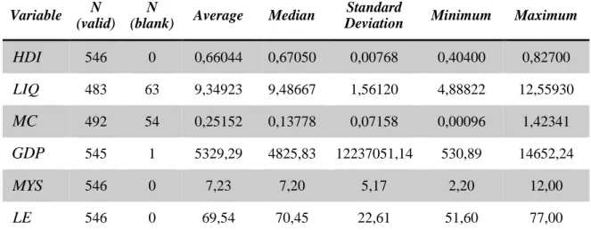
Then, in Table 4, are presented the descriptive statistics of all variables of our model in its original values apart from the liquidity measure that is already presented as the logarithm of the inverse of the Amihud's (2002) illiquidity measure and the market capitalization ratio. The descriptive statistics of the values after applying the logarithms are presented in Appendix 1.