The impact of credit conditions on market liquidity
–
a case for
European stock markets
Miguel Bordadágua Vieira de Brito, nº 865
A Directed Research Project carried out under the supervision of:
Professor João Pedro Pereira
Abstract
The recent financial crisis has drawn the attention of researchers and regulators to the
importance of liquidity for stock market stability and efficiency. The ability of market-makers
and investors to provide liquidity is constrained by the willingness of financial institutions to
supply funding capital. This paper sheds light on the liquidity linkages between the Central
Bank, Monetary Financial Institutions and market-makers as crucial elements to the
well-functioning of markets. Results suggest the existence of causality between credit conditions
and stock market liquidity for the Eurozone between 2003 and 2015. Similar evidence is
found for the UK during the post-crisis period.
1.
Motivation
“Liquidity is the lifeblood of financial markets”1
. It is a complex and multi-faceted
concept. Though widely recognized, to the present, neither a generalized definition of
liquidity nor a single measure capturing all its dimensions has become unanimously accepted.
Nevertheless, a common ground point is that liquidity reflects the easiness of realizing
transactions between agents within the financial system. Hence, liquidity risk arises from the
fact that, in equilibrium, individuals prefer to have liquidity combined with the possibility of
not being liquid at some point in time.
The recent financial crisis has highlighted the importance of liquidity as a precondition
for market completeness. Historically, market liquidity risk has been stable and persistent,
though the occurrence of rare and episodic events revealed the inelasticity of liquidity supply
during crisis. This sudden liquidity “dry-up” may cause large falls in asset prices, not explained by changes in the fundamentals, and augmented by downward spirals: fire sales and
deleveraging as means to meet capital ratios and margin calls.
Graph 1–Eurozone’s Amihud Illiquidity Ratio2
Graph 1 exhibits the Amihud (2002) illiquidity ratio for the Eurozone3 and clearly
illustrates the aforementioned illiquidity spikes for 2008-2009 and 2011-2012, precisely the
periods following the financial and the European sovereign debt crisis, respectively.
1
See Fernandez, F. A. (1999), Liquidity risk. SIA Working Paper
2
Measures the elasticity of stock prices relatively to trading activity, further detail in Section 3
3
For an overall index of four stock market indices: DAX, CAC 40, FTSE MIB and AEX
0 0,0005 0,001 0,0015 0,002 0,0025 0,003 01-2004 05-2004 09-2004 01-2005 05-2005 09-2005 01-2006 05-2006 09-2006 01-2007 05-2007 09-2007 01-2008 05-2008 09-2008 01-2009 05-2009 09-2009 01-2010 05-2010 09-2010 01-2011 05-2011 09-2011 01-2012 05-2012 09-2012 01-2013 05-2013 09-2013 01-2014 05-2014 09-2014 01-2015 05-2015 09-2015
Market liquidity influences a diverse spectrum of macroeconomic indicators as well as
the decision-making of both firms and investors. Næs et al. (2011) evidence that stock market
liquidity is positively correlated with current and future economic growth rates and a robust
predictor of several macroeconomic aggregates. At the firm level, Khapko (2009) concluded
that firms with less liquid stocks tend to have higher debt ratios and are less likely to issue
equity. Amihud and Mendelson (1986) and Pastor and Stambaugh (2003) prove the existence
of a liquidity risk premium for holding illiquid stocks, controlled for other risk factors.
The global financial crisis of 2007-08 has changed the paradigm for the entire financial
system, with consequences for stock market liquidity. Central banks have developed
accommodative policies, through liquidity emergency programs, reduction of policy rates and
the expansion of monetary bases, loan provision to banks or asset purchase programs
(quantitative easing). Initially aimed at reducing financial market distress, these policies also
attempted to stimulate the real economy, although the effects at broad monetary aggregates
were residual since banks preferred to hold reserves. Facing rating downgrades, banks had to
deleverage to comply with higher capital standards and lowered the access to funding to
investors. The current market microstructure is characterized by fragmented large trades, less
structured products, increasing electronic trading and more high-frequency traders, which
reduce transaction costs but still fail to supply liquidity during turmoil periods.
This paper aims to examine the theoretical and empirical relationship between the
Eurozone’s overall credit conditions – the willingness to provide funding liquidity to market intervenients - and stock market liquidity. Credit conditions are assumed to be driven by the
monetary policy stance and resultant interbank market dynamics, changes in monetary and
credit aggregates, as well as the Monetary Financial Institutions (MFIs) balance sheet size and
2.
Literature Review
The literature on stock market liquidity is extensive. Nevertheless, only very recently
studies have investigated the liquidity linkages within the financial intermediation chain,
mainly the existence of feedback mechanisms, as well as spillover effects from monetary
policy and funding liquidity. This section briefly describes the existing literature on stock
market liquidity and details the interactions between drivers of overall credit conditions and
stock market liquidity dimensions.
According to Lybek and Sarr (2002), liquid markets tend to display five distinct and
complementary characteristics: tightness; immediacy; depth; breadth and resiliency. Tightness
gives respect to low transaction costs, while immediacy defines the speed or order execution,
together with the efficiency of trading, clearing and settlement systems. Depth refers to the
existence of abundant orders, below the security price. Breadth means that orders are
numerous and large in volume, with minimal impact on prices. A market is said to be resilient
if new orders flow quickly to order imbalances and attenuate price movements away from
fundamentals.
In a different perspective, some studies have attempted to validate theoretical properties
generally associated with market liquidity. First, commonality in liquidity outlines the fact
that exogenous shocks simultaneously affect all securities in a given market and across
markets, representing a level effect. Further, the “flight-to-quality” effect reports investment allocation changes from small to large caps or ultimately from stocks to bonds, since shocks
are more prone to affect securities with higher volatility, indicating a slope effect. Asymmetry
gives respect to the non-linear response of some liquidity dynamics to exterior innovations,
which are more informative when the risk level is already high. Finally, recall that liquidity
appears to be inelastic in the short-run and is intrinsically related to volatility. Brunnermeier
are mutually reinforcing and sustained by these propositions. Consistent with the latter
predictions, Fontaine and Garcia (2015) observe these same properties for the NYSE, from
1986 to 2012.
Since the genesis of financial markets, intermediaries such as brokers and dealers,
hedge funds and other liquidity suppliers have played a crucial role for market completeness
and the allocation of capital across financial assets. Provided the intermediaries’ wealth is limited, their willingness to provide liquidity will necessarily depend on their ability to obtain
funding. Moreover, funding risk and shocks are contingent on the status quo of credit
conditions. Gromb and Vayanos (2010) document that market liquidity depends on
intermediary capital, namely on the collateral-based financial constraints that limit investment
capacity. Likewise, Johnson (2009) argued about the importance of the stock of liquid capital
to accommodate trade demands and to adjust consumption as a determinant of market
resiliency. Further, Valente (2010) underlines the existence of two extreme regimes: a binding
regime in which funding and market liquidity are positively correlated, and a non-binding
regime without any evidence of correlation, reaffirming the asymmetry property. Adrian and
Shin (2010) describe how intermediaries adjust balance sheets and leverage through
repurchase agreements, so as the direct impact of funding conditions to asset prices and
liquidity.
In the Eurozone, the dynamics between credit conditions and market liquidity are
defined by specific interactions and responsibilities assigned to institutions, intermediaries
and investors. Nikolaou (2009) distinguishes between three liquidity types. First, central bank
liquidity, provided by the ECB, is measured by narrow money M14. Second, funding liquidity
is simply the ability of banks to meet their liabilities and to raise funding in short notice. The
4
liquidity sources of MFIs are deposits, the ECB, the interbank market and the asset market.
Third, the characterization of market liquidity is similar to previous mentioned findings.
Liquidity linkages amongst all types enhance the smooth functioning of the financial
system during normal times, but also represent propagation channels of liquidity risk during
turbulent periods. In fact, a virtuous circle stimulates liquidity flows easily during stable
periods. The ECB, monopoly-provider of liquidity, supplies the liquidity amount that brings
interbank and policy interest rates into equilibrium. Subsequently, liquidity is received by
banks and redistributed accordingly through interbank and asset markets to liquidity-needing
agents. Finally, financially constrained agents demand the necessary amount of liquidity to
satisfy funding necessities, generating a new aggregate liquidity demand to banks and to the
ECB and a new circle begins.
On the opposite, coordination failures among depositors, banks and intermediaries fed
by asymmetric information and incomplete markets, create a vicious illiquidity spiral in the
system. The fragile nature of banks derived from balance sheet maturity mismatch allied to
fears of counterparty credit risk, deposit withdrawals, and ultimately bank runs trigger a
liquidity shortage and the impairment of the interbank market. To avoid liquidation costs,
banks restructure portfolios and enter in fire sales of distressed assets, aggravated by trading
frictions. As in Brunnermeier and Pedersen (2009), the liquidity spiral continues with the
gradual decrease in asset prices and net worth of investors, forcing to further leverage
adjustments in order to meet solvency constraints. Instead, the asset market could have caused
the downward spiral. In response to falling asset prices, investors reduce positions, leading to
higher transaction costs and losses on existing positions, exacerbating funding risk.
Several studies corroborate the existence of such mechanisms in practice. Gagnon and
Gimet (2013) evidence a positive impact on funding and market liquidity following a
and monetary base growth Granger-cause stock market liquidity, while evidence for a
reversed relationship is weak. Chordia et al. (2005) report the monetary policy stance, in the
form of net borrowed reserves, as a driver of stock market liquidity. On the contrary,
Chatterjee (2015) finds evidence that asset market liquidity explains the liquidity creation of
large banks.
Given these points, there is a compelling evidence to assume that the activity of both the
ECB and MFIs is an important factor to determine credit conditions in the Eurozone.
Considering this, it is relevant to assess the decision-making evolution of both intervenients in
the context of pre and post-crisis periods. Until 2008, the ECB has only used conventional
policy instruments. Following the 2008 financial collapse, it has enacted credit support to
financial institutions, several asset purchase programs and, more recently, its first quantitative
easing (QE) program. Nevertheless, the decline in the money multiplier illustrates the
ineffectiveness of monetary policy, particularly relevant when interest rates are at the
zero-lower bound (Valiante, 2015). Most liquidity injected in the financial system has been
accumulated in the form of reserves and in the deposit facility.
Conversely, banks funding practices have also changed in the last decade. In detail, the
recourse to non-core liabilities (i.e. liabilities other than retail deposits) and the ongoing
growth of the outstanding amounts of equity funds units demonstrate the maturation of the
capital-market based “shadow” banking model.
This study contributes to the existing literature by investigating the joint dynamics of
the ECB and MFIs actions on the funding provision to intermediaries and investors,
particularly their subsequent impact on stock market liquidity. Furthermore, the long time
span considers a period of transversal changes for the European financial system. The purpose
of this project disregards the microstructure characteristics of all trading systems considered,
3.
Methodology & Results
In order to accurately describe the dynamics between credit conditions and stock market
liquidity, it is relevant to consider the aforementioned liquidity spirals, potential sources of
endogeneity in the system. Provided there are reasons to expect bidirectional causalities, this
relationship is examined by specifying a Vector Autoregressive (VAR) model. By their linear
structure, VAR models became popular after Sims (1980) proposed them as an improvement
to models with simultaneous equations, and have empirically proven to provide superior
forecasts for macroeconomic and financial time series. However, VAR pitfalls arise in terms
of parsimony, stationarity issues and coefficient interpretation.
To pursue this analysis, four of the most developed European stock markets were
considered, particularly Germany, France, Italy and the Netherlands. The sample includes a
total of 104 stocks included in the actual composition of the DAX, CAC 40, FTSE MIB and
AEX stock indices, respectively. Stocks with non-available data or presenting discontinuous
and outlier values were not considered. All data was retrieved from Bloomberg, the ECB
Statistical Data Warehouse and the Eurostat. The sample period starts in January 2003 and
ends in September 2015, a total of 153 months. In this sense, it is attempted to encompass
different macroeconomic and financial cycles, while avoiding an eventual structural break
with the introduction of the euro in 1999 and less frequent observations for stock market
liquidity variables until the end of 2002.
3.1 Stock Market Liquidity Variables
As pointed in the previous section, instead of reaching a unanimous single-measure and
definition of stock market liquidity, past literature defined a set of characteristics a liquid
asset or market must necessarily exhibit. Combining the research of Lybek and Sarr (2002)
and Nikolaou (2009), three categories of measures were considered: volume-based,
inter-connected and do not incorporate qualitative factors such as market microstructure,
legislative frameworks, payment risks and settlement systems.
First, a volume-based measure is mostly informative about trading activity and concerns
market breadth and depth. Amihud and Mendelson (1986) stated that, in equilibrium, liquid
stocks should be traded more frequently, since the costs of holding illiquid assets could
optimally be spread for longer periods. In this sense, Datar et al. (1998) propose the turnover
rate (TO) measure as a proxy for trading activity. The daily turnover rate of stock i is
computed by dividing the daily number of shares traded by the number of shares outstanding.
𝑇𝑂𝑖,𝑑𝑎𝑦 = # 𝑠ℎ𝑎𝑟𝑒𝑠 𝑜𝑢𝑡𝑠𝑡𝑎𝑛𝑑𝑖𝑛𝑔# 𝑠ℎ𝑎𝑟𝑒𝑠 𝑡𝑟𝑎𝑑𝑒𝑑𝑖,𝑑𝑎𝑦𝑖,𝑑𝑎𝑦× 100 (1)
Second, indicators of price-impact costs aim to assess market resiliency and speed of
price discovery. Particularly, they capture the price responsiveness to order flow movements
since, intuitively, more liquid assets should be less sensitive to large and numerous orders.
Orderly and resilient markets provide greater price continuity and lower volatility, key
indicators of liquidity and critical for investment decision-making. The Amihud’s (2002) illiquidity ratio (AMIHUD) ascertains an elasticity dimension of liquidity, that is, the
response of returns to 1 euro of trading volume. Despite being highly correlated with market
capitalization and inflation, many researchers advocate its adequacy as a price impact
measure. Contrary to the turnover rate, this measure is negatively related to liquidity and
given by the ratio between the absolute daily return of stock i divided by the respective traded
value in euro.
𝐴𝑀𝐼𝐻𝑈𝐷𝑖,𝑑𝑎𝑦 = 𝑇𝑟𝑎𝑑𝑒𝑑 𝑣𝑎𝑙𝑢𝑒 𝑖𝑛 𝑒𝑢𝑟𝑜|𝑅𝑒𝑡𝑢𝑟𝑛𝑖,𝑑𝑎𝑦|
𝑖,𝑑𝑎𝑦× 10
6 (2)
Third, transaction costs may be viewed as the price required by market-makers (brokers
and dealers) for providing liquidity services and immediacy of execution, thus representing
spread (BID_ASK) is the most widely used measure. The spread depicts the sum of the
buying premium and the selling concession and is computed as the ratio of the difference
between the daily ask and bid price to the last price.
𝐵𝐼𝐷_𝐴𝑆𝐾𝑖,𝑑𝑎𝑦= 𝐴𝑠𝑘−𝑝𝑟𝑖𝑐𝑒𝐿𝑎𝑠𝑡−𝑝𝑟𝑖𝑐𝑒𝑖,𝑑𝑎𝑦−𝐵𝑖𝑑−𝑝𝑟𝑖𝑐𝑒𝑖,𝑑𝑎𝑦
𝑖,𝑑𝑎𝑦 × 2 (3)
A preliminary analysis to the daily data for market liquidity measures exposed several
anomalous and extreme values which could undermine the final results. Hence, for each stock
index two filters were applied by deleting daily index indicators formed by less than 10
observations of individual stocks and months with less than 10 trading days available were
also removed. To aggregate each liquidity measure (MLIQ), the daily average of the liquidity
measure for all individual stocks in the index is computed5. Finally, daily figures are
equally-averaged to obtain monthly-level indicators6, which subsequently are aggregated to an overall
level by estimating a weighted average using the number of stocks corresponding to each
index as the weights assigned7.
3.2Credit Conditions Variables
Similarly, credit conditions cannot be assessed based on a single indicator. Instead,
three major factors are considered: interbank market credit risk, the monetary policy
effectiveness to stimulate credit creation, and the composition of bank liabilities.
The interbank market is undoubtedly the major source of liquidity for MFIs. In this
sense, a measure of the perceived risk and creditworthiness in this market may provide an
accurate proxy of funding liquidity. As suggested by Brunnermeier (2009), market observers
often focus on the TED spread, the difference between the 3-month U.S dollar LIBOR8 and
5
𝑀𝐿𝐼𝑄𝑖𝑛𝑑𝑒𝑥,𝑑𝑎𝑦 = # 𝑠𝑡𝑜𝑐𝑘𝑠1
𝑖𝑛𝑑𝑒𝑥,𝑑𝑎𝑦× ∑ 𝑀𝐿𝐼𝑄𝑠𝑡𝑜𝑐𝑘,𝑑𝑎𝑦, 𝑓𝑜𝑟 𝑠𝑡𝑜𝑐𝑘 = 1, … , #𝑠𝑡𝑜𝑐𝑘𝑠 ∧ #𝑠𝑡𝑜𝑐𝑘𝑠 ≥ 10
6
𝑀𝐿𝐼𝑄𝑖𝑛𝑑𝑒𝑥,𝑚𝑜𝑛𝑡ℎ= # 𝑡𝑟𝑎𝑑𝑖𝑛𝑔 𝑑𝑎𝑦𝑠1𝑖𝑛𝑑𝑒𝑥,𝑚𝑜𝑛𝑡ℎ× ∑ 𝑀𝐿𝐼𝑄𝑖𝑛𝑑𝑒𝑥,𝑑𝑎𝑦, 𝑓𝑜𝑟 𝑑𝑎𝑦 = 1, … , #𝑡𝑟𝑎𝑑𝑖𝑛𝑔 𝑑𝑎𝑦𝑠 ∧
#𝑡𝑟𝑎𝑑𝑖𝑛𝑔 𝑑𝑎𝑦𝑠 ≥ 10
7
𝑀𝐿𝐼𝑄𝑜𝑣𝑒𝑟𝑎𝑙𝑙,𝑚𝑜𝑛𝑡ℎ= # 𝑠𝑡𝑜𝑐𝑘𝑠𝑜𝑣𝑒𝑟𝑎𝑙𝑙,𝑚𝑜𝑛𝑡ℎ1 × ∑(𝑀𝐿𝐼𝑄𝑖𝑛𝑑𝑒𝑥,𝑚𝑜𝑛𝑡ℎ× #𝑠𝑡𝑜𝑐𝑘𝑠𝑖𝑛𝑑𝑒𝑥,𝑚𝑜𝑛𝑡ℎ) , 𝑓𝑜𝑟 𝑖𝑛𝑑𝑒𝑥 = 1, 2, 3, 4
8
the 3-month U.S Treasury Bills rate. The spread measures the difference in yields between
unsecured top-rated interbank loans and government seemingly ‘riskless’ credits, though after the financial crisis researchers often disagree on its definition and content. Although both
rates tend to co-move, a TED spread widening is characteristic of a destabilizing spiral
predictor, impacting both interbank liquidity and credit availability. To estimate the Eurozone
analogous TED spread (TED_EZ), the difference between the 3-month Euribor9 and the
3-month zero-coupon German bund is computed. The German bund is frequently used as the
risk-free rate benchmark for the Eurozone.
𝑇𝐸𝐷_𝐸𝑍𝑚𝑜𝑛𝑡ℎ = 3𝑀 𝐸𝑈𝑅𝐼𝐵𝑂𝑅𝑚𝑜𝑛𝑡ℎ− 3𝑀 𝐺𝑒𝑟𝑚𝑎𝑛 𝐵𝑢𝑛𝑑𝑚𝑜𝑛𝑡ℎ (4)
The volume of money supply is the result of the transmission mechanism interaction
between the central bank, the banking sector and non-financial intermediaries. In particular,
money creation is ultimately linked to credit expansion and to the intermediation capacity of
MFIs through the credit-deposit multiplier process.
A traditional method to assess the monetary policy effectiveness and credit development
is through the money multiplier approach, which presumes that broad money M3 is solely
driven by narrow money M1 and the money multiplier (MM). Nonetheless, this proposition
assumes that the behaviour of banks and the money-holding sector will respond in a
predictable way to shocks in M1. By contrast, after 2008, in the context of extreme
uncertainty regarding bank balance sheet soundness in the interbank markets, banks
responded to the ECB liquidity stimuli by increasing reserve holdings beyond the minimum
requirement. To demonstrate this point, it may be interesting to analyse the decomposition of
the money multiplier:
𝑀𝑜𝑛𝑒𝑦 𝑀𝑢𝑙𝑡𝑖𝑝𝑙𝑖𝑒𝑟 = 1+ 𝐷𝐶 𝑅 𝐷+𝐷𝐶
(5)
9
Where C/D is the currency-to-deposits ratio (CUR_DEP) and R/D the
reserves-to-deposits ratio (RES_DEP)10.
As can be derived, changes in MM are negatively driven by increases in the
currency-to-deposits ratio and in the reserves-currency-to-deposits ratio. Intuitively, if currency holders retain
more money as currency and banks hold more reserves, the multiplier effect through loans
and deposits is reduced. Positive innovations in the reserves-to-deposits ratio underpin that
MFIs are less willing to provide funding liquidity. On the other hand, the currency-to-deposits
ratio may signal a twofold effect on stock market liquidity. The decision to hold currency
instead of depositing or investing can be either caused by good credit conditions in the form
of very-low interest rates or by a higher perception of risk and preference for liquidity. In
short, both components of MM are included in the model to retain the informative power of
both variables for coherence.
At last, credit availability may be associated to the MFIs balance sheet size and
composition not scrutinized by monetary aggregates. In a bank-based economy, MFIs are the
most important financial intermediaries to which retail deposits (core liabilities) have been the
main source of funding. Nonetheless, Hahm et al. (2013) report that whenever credit is
growing at a faster pace compared to deposit levels, banks turn to other funding sources. For
this reason, the amount of MFI non-core liabilities is a prime indicator of higher credit
availability and inherent lower external finance premiums, necessary conditions for easing
credit conditions.
The current systematic low-margin banking environment is leading to gradual
deleveraging, thus benefiting the capital-market banking model. Namely, the on-going rise of
the asset management activity in Europe has posed a good source of collateral for the repo
10
C denotes banknotes in circulation, D denotes deposits in M3 (overnight deposits + deposits up to 2 years + deposits redeemable up to 3 months + deposits up to 2 years and redeemable up to 3 months) and R represents
markets, key funding instruments for market-makers. All in all, to consider the impact of both
factors for overall credit conditions, a final variable is included:
𝑁𝐶𝑂𝑅𝐸𝑚𝑜𝑛𝑡ℎ= 𝑙𝑛(𝑁𝑜𝑛 − 𝑐𝑜𝑟𝑒 𝑙𝑖𝑎𝑏.𝑚𝑜𝑛𝑡ℎ11+ 𝐸𝑞𝑢𝑖𝑡𝑦 𝑓𝑢𝑛𝑑 𝑠ℎ𝑎𝑟𝑒𝑠/𝑢𝑛𝑖𝑡𝑠𝑚𝑜𝑛𝑡ℎ) (6)
Where ln represents the natural logarithm and Non-core liab. the outstanding amount of
MFIs non-core liabilities to which the outstanding amount of equity and non-money-market
funds shares/ units is added.
3.3Adjustment of Time Series
3.3.1 Control Variables
As mentioned, the relationship between stock market liquidity and main financial and
macroeconomic indicators has been thoroughly documented. Under those circumstances,
failing to control for these exogenous factors may lead to inconsistent results. Thus, following
Chordia et al. (2005), the weighted-average of monthly returns (MRET) and monthly standard
deviation of daily stock returns (MSTDEV) are introduced, again considering the number of
stocks as weights allocated to each stock index. Since the short-term business cycle and price
evolution developments also represent crucial information criteria for the ECB, the annual
rate of change of the Euro Area Harmonised Index of Consumer Prices (IR)12 as a proxy for
inflation and the Euro Area Industrial Production Index (IPI)13 are included. All four
indicators are incorporated as exogenous variables.
3.3.2 Stationarity Tests
According to Lütkepohl (2005) every stationary, strictly non-deterministic process can
be approximated by a VAR model. For this reason, dealing with non-stationary variables may
result in spurious regressions, inconsistent estimators and subjacent incorrect causality
test-statistics. Provided this, to ensure that all variables are stationary and of the same order of
11
Non-core liabilities = debt securities held + money market funds shares/ units + debt securities issued + remaining liabilities + external liabilities, extra Euro Area
12
Euro Area actual composition (19 countries)
13
integration, Augmented Dickey-Fuller (ADF) tests14 were performed for all variables. Only
for the currency-to-deposits ratio (CUR_DEP) and the inflation rate (IR), the null hypothesis
of a unit root was not rejected at a 5% significance level. Therefore, first differences of both
indicators were taken, dCUR_DEP and dIR, respectively.
3.4 Descriptive Statistics and Correlation Matrix
Table 2 presents summary statistics for all variables during the entire period covered by
the sample. As projected, the time interval considered for this analysis comprises different
financial and business cycles, emphasized by disperse values observed in the TED spread,
monthly stock returns and in the industrial production index.
Likewise, Table 3 shows pairwise correlation coefficients between all variables. The
high negative correlation between non-core liabilities and the Amihud’s ratio indicates that the first may perhaps be a good estimator of the latter. Also, the market standard deviation is
positively correlated with the turnover rate, the Amihud’s ratio and the TED spread, meaning
that these variables could indicate market’s perception of increasing risk.
3.5 Model Specification and Validation
Accordingly, the following VAR model of order p is specified:
𝑦𝑡= 𝐴𝑌𝑡−1+ 𝐵0𝑥𝑡+ 𝑢𝑡15 (7)
The procedure to select the optimal lag length must contemplate the consistency of the
estimators and guarantee that innovations follow a White Noise process. Ultimately, it is
implausible to satisfy both criteria simultaneously and avoid the trade-offs involved in this
decision. For this purpose, the Akaike (AIC) and the Schwarz-Bayesian information criterion
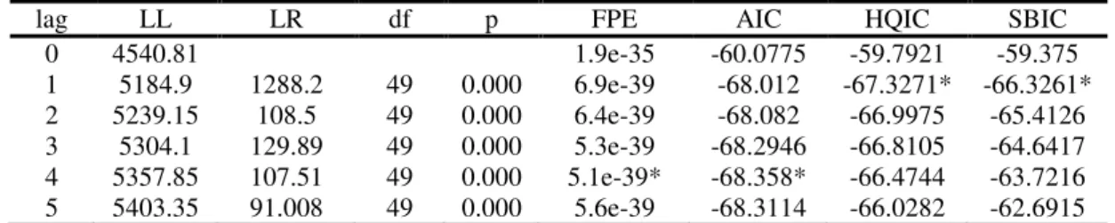
(BIC) were estimated from lags 1 to 516. The lag length that minimizes the AIC is 4 whilst the
BIC is optimal for order 1, in line with the more conservative approach of the first measure.
14
ADF test results are presented in Table 4 of the Appendix
15
yt is a vector of the 7 endogenous variables (TO, AMIHUD, BID_ASK, TED_EZ, dCUR_DEP, RES_DEP
and logNCORE); A is a matrix of coefficients for endogenous variables; Yt-1 is a matrix of past values of all
endogenous variables; B0 a matrix of coefficients for exogenous variables and the constant term; xt a vector of
exogenous variables and a constant term; and ut a vector of residuals 16
As means to retain a simpler and more parsimonious structure, a VAR (1) model is therefore
chosen.
Nevertheless, in order to secure the whiteness of model residuals, the
Lagrange-Multiplier (LM) test was performed for the null hypothesis of no residual autocorrelation of
order 1 and rejected at a 5% significance level. To repeat the test in an ascending order, one
more lag is added to the VAR model17. The test sequence was terminated at the lag length of
4, for which the null of no residual autocorrelation was not rejected. In short, specifying a
VAR (4) model satisfies the AIC and retains the asymptotic properties of the estimators.
Before performing causality and structural analyses of the VAR model, the initial
assumption of stability must be validated. Lutkepohl (2005) states that a VAR model of order
p is stable if all eigenvalues of the A coefficient matrix have no roots within or on the unit
circle, meaning that impulse response functions (IRFs) have known interpretations. After
performing the test18, the results conclude that all the eigenvalues lie inside the unit circle,
thus the referred VAR model is stable.
3.6 Causality Analysis – Granger-causality tests
To interpret the results of the estimated VAR (4) model, Granger-causality tests19 are
conducted to assess the existence of a statistically significant impact of credit conditions on
stock market liquidity and vice-versa. This concept advocates that if variable x
Granger-causes variable y, then past values of x contain information to improve the estimates of y
beyond past values of y alone. The null hypothesis states that the credit conditions (market
liquidity) variable does not Granger-cause the market liquidity (credit conditions) variable.
Table 1 reports Chi-square test-statistics and p-values for all the tests, divided by the two
possible directions of causality.
17
Results of the LM Test are presented in Table 6 of the Appendix
18
Results presented in the Annex
19
Table 1 – Granger-causality Tests
All data considered in the sample was retrieved from Bloomberg, the ECB Statistical Data Warehouse and the Eurostat from January 2003 to September 2015. Market liquidity variables included observations from 104 stocks currently traded in the DAX, CAC 40, FTSE MIB and AEX stock indices. Stocks with non-available data or presenting anomalous values were not considered.
Credit Conditions Market Liquidity
TO AMIHUD BID_ASK
(i) – Credit Conditions (row) Market Liquidity (column)
H0: Credit Conditions measure (row) does not Granger-cause the Market Liquidity measure (column)
TED_EZ 15.612*** (0.004)
1.080 (0.897)
12.579** (0.014) dCUR_DEP 12.024**
(0.017)
51.723*** (0.000)
5.900 (0.207) RES_DEP 6.057
(0.195)
4.782 (0.310)
16.671*** (0.002) logNCORE 13.466***
(0.009)
9.800** (0.044)
2.480 (0.649) (ii) – Market Liquidity (column) Credit Conditions (row)
H0: Market Liquidity measure (column) does not Granger-cause the Credit Conditions measure (row)
TED_EZ 5.602
(0.231)
8.038* (0.090)
4.194 (0.380) dCUR_DEP 5.487
(0.241)
36.644*** (0.000)
4.764 (0.312) RES_DEP 2.389
(0.665)
6.409 (0.171)
93.843*** (0.000) logNCORE 5.380
(0.250)
5.912 (0.206)
3.186 (0.527) Note: P-values in parenthesis. *, ** and *** denote 10%, 5% and 1% significance levels
Overall, the results of the Granger-causality tests corroborate that credit conditions
Granger-cause market liquidity in all its three dimensions. Apart from certain exceptions,
there is little evidence of a bidirectional causal relationship. In detail, the TED spread for the
Eurozone, the currency-to-deposits ratio and the non-core liabilities of MFIs seem to be
informative to predict simultaneously two market liquidity variables, whereas the
reserves-to-deposits ratio only has a statistically significant impact on the bid-ask spread. Conversely, the
Amihud’s illiquidity ratio and the bid-ask spread Granger-cause the currency-to-deposits and the reserves-to-deposits ratios, respectively.
3.7 Structural Analysis – Impulse Response Functions
The causality analysis provided by the Granger-causality tests does not tell the entire
story about the interactions between the variables. As results are based on single equation
coefficients, they do not consider the joint dynamics in the VAR system. Hence, a clearer
one-time, unit standard deviation, positive shock to the impulse variable on the present and future
values of the response variable in a higher dimensional system.
Before conducting this procedure, some key issues must be addressed. First, Luktepohl
(2005) asserts that IRFs are not statistically different from 0 if the impulse variable does not
Granger-cause the response variable. Second, IRFs assume that a shock occurs only in one
variable at a time. In order to ensure that shocks and independent, residuals are
orthogonalized by a Cholesky decomposition. At last, the accuracy of results is sensitive to
the ordering of variables in the VAR estimation. The Wold causal ordering determines that
variables with greater transversal influence should be placed first. Following
Fernández-Amador et al. (2013), monetary and credit variables are placed before market liquidity
indicators.
Graphs 2-10 depict the one Cholesky standard deviation innovation impact on the
response variable of interest for all significant Granger-causality interactions20.
20
The remaining IRFs are presented in the Annex
Graph 2– Response of TO to TED_EZ Graph 3 –Response of TO to dCUR_DEP
Graph 4– Response of TO to logNCORE Graph 5 – Response of AMIHUD to
dCUR_DEP
Overall, the IRF results are the empirical reflex of the financial theory and emphasize
how changes in several aspects of credit conditions directly impact various dimensions of
stock market liquidity. With certain exceptions, the impact of explanatory variables is only
significant in the short-term, mainly on the first 3 months.
Additionally, the signs of all IRFs confirm the hypotheses presented in previous
sections. The TED spread has a negative effect on the turnover rate, while at the same time a
positive effect on the bid-ask spread after a few months, hence positive shocks to this variable
exercise a negative influence on market liquidity. As predicted, the currency-to-deposits has a
Graph 6 – Response of AMIHUD to
logNCORE
Graph 7 – Response of BID_ASK to
TED_EZ
Graph 8 – Response of BID_ASK to
RES_DEP
Graph 9 – Response of dCUR_DEP to
AMIHUD
Graph 10– Response of RES_DEP to BID_ASK
dual effect: negative on the turnover rate, lowering trading activity and positive to reduce
price impact costs hereby represented by the Amihud’s illiquidity ratio. Further, the bid-ask spread response to a shock in the reserves-to-deposits ratio is positive, proving that if MFIs
retain higher reserves intermediaries will have lower funding liquidity and therefore reduce
their market-making activity. Moreover, increasing non-core liabilities significantly raises the
turnover rate on the short-term, though has a lasting and structural effect on reducing the
Amihud ratio. The latter result may indicate that financial intermediaries and investors do not
have an immediate reaction to this variable, but instead tend to wait to adjust their balance
sheets and funding constraints. Lastly, positive innovations in the Amihud ratio and the
bid-ask spread have a positive impact on the money multiplier, by reducing the
currency-to-deposits and the reserves-to-currency-to-deposits ratios, respectively. This bidirectional causality effect
proves the existence of a liquidity spiral only extended to the money multiplier level.
3.8 Robustness Check – a similar model for the United Kingdom
The aforementioned results are cemented on liquidity interactions within the bank-based
financing structure of the Eurozone. For a market-centric economy like the United Kingdom
(UK), the results may not hold. In fact, the ECB and the Bank of England (BoE) have differed
on balance sheet composition and monetary policy intervention after 2008, as the BoE
responded with greater quantities of bond purchases. Also, the interactions between agents in
a different and more homogenous monetary financial system may lead to different
conclusions. In this context, the previous model is replicated for the UK during the post-crisis
period21. To ensure variable comparability, the data set starts in January 2010 and ends in
September 2015. Stock market liquidity variables were retrieved by stocks currently listed on
the FTSE 100.
21
Granger-causality test results are presented in Table 7, and confirm the hypothesis of
causality between credit conditions and stock market liquidity for the UK, while proof for the
hypothesis of reciprocal causality is less evident22. Accordingly, the IRFs plotted for
significant causal relationships in Graphs 11-14 yield similar results relatively to the
Eurozone. Positive innovations in the TED spread and the reserves-to-deposits are followed
by increases in the Amihud illiquidity ratio in the short-term. Moreover, the
reserves-to-deposits ratio growth has a negative impact on the turnover rate, while the TED spread
widening raises the bid-ask spread during a more prolonged period. To conclude, it is
interesting to notice that both the currency-to-deposits ratio and MFI non-core liabilities fail
to impact any of the stock market liquidity dimensions. Provided the more market-oriented
action of the BoE, the impact of both variables on stock market liquidity is found to be less
significant.
22
At a 5% significance level, only the bid-ask spread (BID_ASK_UK) is found to Granger-cause non-core liabilities (dNCORE_UK)
Graph 11 – Response of TO_UK to
dRES_DEP_UK
Graph 12 – Response of AMIHUD_UK to
TED_UK
Graph 13 – Response of AMIHUD_UK to
dRES_DEP_UK
Graph 14 – Response of BID_ASK_UK to
TED_UK
4.
Conclusion
This paper examines the interplay relationship between the Central Bank and MFIs to
determine credit conditions and the succeeding impact on stock market liquidity in the
Eurozone from 2003 to 2015. In order to provide a fairly comprehensive picture of both
concepts, several measures were integrated in the analysis and controlled for macroeconomic
and financial variables. Further, the time span considered aims to enact the different behavior
between agents during normal and turmoil periods. To test the model robustness, a similar
procedure was conducted for a different monetary area, the UK.
The main results confirm the initial premise and can be summarized as follows. First,
credit conditions represented by the interbank market sentiment, the monetary policy
effectiveness and the MFIs financing structure jointly determine stock market liquidity. In
fact, all IRF signs corroborate the hypothesis that easing credit conditions affect positively all
dimensions of market liquidity. Second, evidence for the existence of liquidity spirals and
bidirectional causalities is rather weak and only found at the money multiplier level. Third,
even though the main results are verified for the UK, the impact of the currency-to-deposits
ratio and the non-core liabilities is not statistically significant in this case.
This study leaves several doors open for future research. To start with, the impact of
credit conditions on other asset markets (e.g. bond and derivatives markets) has yet to be
investigated. Also, this relationship can be tested for European peripheral countries,
particularly after the sovereign debt crisis. Bearing in mind the current transformations and
challenges affecting financial markets, further analyses can incorporate the impact of
regulations, capital standards and the increasing participation of high frequency traders. The
possible existence of a flight-to-quality effect during the current QE program enacted by the
ECB could also be assessed. Finally, an event study following the impact of ECB meeting
5.
References
Adrian, T., and H. Shin. 2010. “Liquidity and Leverage.” Journal of Financial Intermediation, Vol. 19: 418-437
Amihud, Y. 2002. “Illiquidity and Stock Returns: Cross-section and time series effects.” Journal
of Financial Markets, Vol. 5:31-56
Amihud, Y., and H. Mendelson. 1986. “Liquidity and Stock Returns.” Financial Analysts Journal, Vol. 42:43-48
Brunnermeier, M. 2009. “Deciphering the Liquidity and Credit Crunch 2007-2008.” Journal of
Economic Perspectives, Vol. 23: 77-100
Brunnermeier, M. K., and L. Pedersen. 2009. “Market Liquidity and Funding Liquidity.” Review
of Financial Studies, Vol. 22: 2201-2238
Chatterjee, U. K. 2015. “Bank Liquidity Creation and Asset Market Liquidity.” Journal of
Financial Stability, Vol. 18: 19-153
Chordia, T., A. Sarkar, and A. Subrahmanyam. 2005. “An Empirical Analysis of Stock and Bond
Market Liquidity.” Review of Financial Studies, Vol. 18: 85-129
Datar, V. T., N. Y. Naik, and R. Radcliffe. 1998. “Liquidity and Stock Returns: an Alternative
Test.” Journal of Financial Markets, Vol. 1(2): 203-219
Fernandez, F. A. 1999. “Liquidity Risk.” Working Paper, SIA
Fernández-Amador, O., M. Gächter, M. Larch, and G. Peter. 2013. “Does Monetary Policy
Determine Stock Market Liquidity? New Evidence from the Eurozone.” Journal of
Empirical Finance, Vol. 21: 54-68
Fontaine, J., R. Garcia, and S. Gungor. 2015. “Funding Liquidity, Market Liquidity and the
Cross-section of Stock Returns.” Working paper, Bank of Canada
Gagnon, M., and C. Gimet. 2013. “The Impacts of Standard Monetary and Budgetary Policies on
Liquidity and Financial Markets: International Evidence from the Credit Freeze Crisis.”
Journal of Banking and Finance, Vol. 37(11): 4599-4614
Gromb, D., and D. Vayanos. 2010. “A Model of Financial Market Liquidity Based on
Intermediary Capital.” Journal of the European Economic Association, Vol. 8: 456-466
Hahm, J., H. Shin, and K. Shin. 2013. “Non-core Bank Liabilities and Financial Vulnerability.”
Journal of Money, Credit and Banking, Vol. 45(1): 3-36
Johnson, T. C. 2009. “Liquid Capital and Market Liquidity.” The Economic Journal, Vol. 119:
1374-1404
Khapko, M. 2009. “The Impact of Stock Market Liquidity on Corporate Finance Decisions.”
Master of Arts in Economics thesis, Central European University
Lütkepohl, H. 2005. New Introduction to Multiple Time Series Analsysis. New York: Springer
Næs, R. J. A. Skeltorp, and B. Ødegaard. 2011. “Stock Market Liquidity and the Business
Cycle.” The Journal of Finance, Vol. 66(1): 139-176
Nikolaou, K. 2009. “Liquidity (Risk) Concepts: Definitions and Interactions.” Working Paper,
European Central Bank
Pastor, L., and R. F. Stambaugh. 2003. “Liquidity Risk and Expected Stock Returns.” Journal of
Political Economy, Vol. 113: 642-685
Lybek, T., and A. Sarr. 2002. “Measuring Liquidity in Financial Markets.” Working Paper,
International Monetary Fund
Sims, C. 1980. “Macroeconomics and Reality.” Econometrica, Vol. 48(1): 1-48
Valente, G. 2010. “Market Liquidity and Funding Liquidity: an Empirical Investigation.”
Working Paper, Hong Kong Institute for Monetary Research
6.
Appendix
Table 2 – Summary Statistics
Observations Mean St. Deviation Min Median Max TO 153 0.005508 0.001038 0.003815 0.005367 0.010156 AMIHUD 153 0.000851 0.000886 0.000188 0.000525 0.006338 BID_ASK 153 0.004690 0.006385 0.001350 0.002768 0.058982 TED_EZ 154 0.003888 0.004601 -0.000300 0.002100 0.028200 dCUR_DEP 153 0.000221 0.000504 -0.002824 0.000227 0.002781 RES_DEP 153 0.027101 0.014807 0.000014 0.019581 0.077107 logNCORE 153 13.954049 0.126956 13.607562 14.013605 14.139865
MRET 153 0.004442 0.049959 -0.153848 0.012710 0.154600 MSTDEV 153 0.012732 0.006727 0.004862 0.011007 0.051116 dIR 154 -0.000149 0.002614 -0.011000 0.000000 0.008000 IPI 152 102.60342 8.580147 75.70000 103.25000 121.98000
Table 3 – Correlation Matrix
Table 4 – Augmented Dickey-Fuller Stationarity Tests
Variable / Null Hypothesis H0: Unit Root
Turnover Rate (TO) -6.586*** (0.000) Amihud Illiquidity Ratio
(AMIHUD)
-4.012*** (0.001) Effective Bid-Ask Spread
(BID_ASK)
-5.895*** (0.000)
Eurozone TED Spread (TED_EZ) -3.802*** (0.003) Currency to Deposit Ratio
(dCUR_DEP)
-11.344*** (0.000) Reserves to Deposit Ratio
(RES_DEP)
-3.379*** (0.012) Note: P-values in parenthesis. *, ** and *** denote 10%, 5% and 1% significance level
TO AMIHUD BID_ASK TED_EZ dCUR_DEP RES_DEP logNCORE
TO 1.000
AMIHUD 0.0392 1.000
BID_ASK 0.0074 0.0812 1.000
TED_EZ 0.4377 0.1300 0.2897 1.000
dCUR_DEP -0.0043 0.1480 0.0112 0.1181 1.000
RES_DEP 0.0408 -0.0798 0.4695 0.3421 -0.0874 1.000
logNCORE 0.2133 -0.6437 0.0967 0.4134 -0.2427 0.3405 1.000
MRET -0.3782 -0.0937 -0.1320 -0.3391 0.0465 -0.0646 -0.1301 MSTDEV 0.5548 0.4464 0.1989 0.7582 0.2180 0.2625 0.1327
dIR -0.0310 -0.1252 -0.0074 -0.2455 -0.0563 -0.1201 0.0173 IPI 0.3925 -0.1834 -0.0497 0.0138 -0.1427 -0.1578 0.1296
MRET MSTDEV dIR IPI
MRET 1.000
MSTDEV -0.4548 1.000
Variable / Null Hypothesis H0: Unit Root
MFIs Non-Core Funding Liquidity (logNCORE)
-2.672* (0.079)
Stock Market Return (MRET) -10.676*** (0.000) Stock Market Standard Deviation
(MSTDEV)
-4.919*** (0.000)
Inflation Rate (dIR) -10.450*** (0.000)
Industrial Production Index (IPI) -9.342*** (0.000)
Note: P-values in parenthesis. *, ** and *** denote 10%, 5% and 1% significance levels
Table 5 – VAR Order Selection Criteria
lag LL LR df p FPE AIC HQIC SBIC 0 4540.81 1.9e-35 -60.0775 -59.7921 -59.375 1 5184.9 1288.2 49 0.000 6.9e-39 -68.012 -67.3271* -66.3261* 2 5239.15 108.5 49 0.000 6.4e-39 -68.082 -66.9975 -65.4126 3 5304.1 129.89 49 0.000 5.3e-39 -68.2946 -66.8105 -64.6417 4 5357.85 107.51 49 0.000 5.1e-39* -68.358* -66.4744 -63.7216 5 5403.35 91.008 49 0.000 5.6e-39 -68.3114 -66.0282 -62.6915 Note: * denote optimal values for each criterion
Table 6 – Lagrange-Multiplier Test for Residual Autocorrelation
Lag Chi-Square Statistic df Prob. > Chi-Square Statistic
1 106.0072 49 0.00000
2 83.4792 49 0.00155
3 70.8867 49 0.02207
4 54.7008 49 0.26706
H0: No autocorrelation at lag order
Table 7 – UK Model Granger-causality Tests
Credit Conditions Market Liquidity
TO_UK AMIHUD_UK BID_ASK_UK (i) – Credit Conditions (row) Market Liquidity (column)
H0: Credit Conditions measure (row) does not Granger-cause the Market Liquidity measure (column)
TED_UK 1.560
(0.458)
5.706* (0.058)
7.529** (0.023) dCUR_DEP_UK 4.708*
(0.095)
4.098 (0.129)
0.726 (0.695) dRES_DEP_UK 8.546**
(0.014)
12.134*** (0.002)
3.464 (0.177) dNCORE_UK 0.193
(0.908) n/a
2.304 (0.316) (ii) – Market Liquidity (column) Credit Conditions (row)
H0: Market Liquidity measure (column) does not Granger-cause the Credit Conditions measure (row)
TED_UK 0.622
(0.733)
0.608 (0.738)
0.552 (0.759) dCUR_DEP_UK 0.017
(0.992)
1.615 (0.446)
0.712 (0.700) dRES_DEP_UK 1.164
(0.559)
1.795 (0.407)
3.826 (0.148) dNCORE_UK 1.457
(0.483)
0.940 (0.625)