(will be inserted by the editor)
QED and relativistic corrections in superheavy elements
P. Indelicato1, J.P. Santos2, S. Boucard1, and J.-P. Desclaux3
1 Laboratoire Kastler Brossel, ´Ecole Normale Sup´erieure; CNRS; Universit´e P. et M. Curie - Paris 6
Case 74; 4, place Jussieu, 75252 Paris CEDEX 05, France e-mail:[email protected]
2 Centro de F´ısica At´omica and Departamento de F´ısica, Faculdade de Ciˆencias e Tecnologia, Universidade Nova de Lisboa,
Monte de Caparica, 2829-516 Caparica, Portugal
3 15 Chemin du Billery, 38360 Sassenage, France e-mail: [email protected]
Received: May 31, 2007/ Revised version: date
Abstract. In this paper we review the different relativistic and QED contributions to energies, ionic radii, transition probabilities and Land´eg-factors in super-heavy elements, with the help of the MultiConfigura-tion Dirac-Fock method (MCDF). The effects of taking into account the Breit interacMultiConfigura-tion to all orders by including it in the self-consistent field process are demonstrated. State of the art radiative corrections are included in the calculation and discussed. We also study the non-relativistic limit of MCDF calculation and find that the non-relativistic offset can be unexpectedly large.
PACS. 31.30.Jv – 31.25.Eb – 31.25.Jf – 32.70.Cs
1 Introduction
In the last decades, accelerator-based experiments at GSI and Dubna have lead to the discovery of super-heavy ele-ments up toZ = 116 and 118 [1] (for a recent review see [2]). Considerable theoretical work has been done to pre-dict the ground configuration and the chemical properties of those superheavy elements. Relativistic Hartree-Fock has been used to predict the ground configuration proper-ties of superheavy elements up to Z = 184 in the early 70’s [3,4]. The Multiconfiguration Dirac-Fock (MCDF) method was used to predict orbital properties of elements up toZ= 120 [5], electron binding energies up toZ= 118 [6,7], and K-shell and L-shell ionization potentials for the superheavy elements with Z = 112, 114, 116, and 118 [8]. Ionization potential and radii of neutral and ionized bohrium (Z = 107) and hassium (Z = 108) have been evaluated with large scale MCDF calculations [9]. Kaldor and coworkers have employed the relativistic coupled-cluster method to predict ground state configuration, ionization potential, electron affinity, binding energy of the negative ion of several elements withZ ≥100 [10,11,12,13,14,15, 16,17].
Very recently, laser spectroscopy of several fermium (Z= 100) transitions has been performed, the spectroscopy of nobelium (Z = 102) is on the way [18,19,20], and large scale MCDF calculations of transition energies and rates have been performed by several authors for super-heavy elements with Z = 100 [18,21], Z = 102 [21] and
Z = 103 [22], which are in reasonable agreement with the fermium measurements.
Send offprint requests to: P. Indelicato
There are however many unanswered questions, that need to be addressed in order to assess the accuracy and the limit of current theoretical methods. For inner-shells, or highly ionized systems, QED effects must be very strong in superheavy elements, where the atomic number Z ap-proaches the limit Zα → 1 (α = 1/137.036 is the fine structure constant), at which the point-nucleus Dirac equa-tion eigen-energies become singular for all s1/2 and p1/2 states (the energy depends on
q
j+1 2
2
−(Zα)2, where
j is the total angular momentum). This means that all QED calculations must be performed for finite nuclei, and to all orders in Zα. QED calculations for outer-shell are very difficult. At present, only the simplest one-electron, one-loop diagrams can be calculated, using model poten-tials to account for the presence of the other electrons. The evaluation of many-body effects, that remains large for neutral and quasi-neutral systems, is also made very difficult by the complex structure of these atoms, in which there may be several open shells. In that sense, meth-ods based on Relativistic Many-Body Perturbation theory (RMBPT) and MCDF methods are complementary. The former one usually allowing for more accurate results, but limited to (relativistic) closed shell systems minus one or plus one or at most two electrons, while the latter is com-pletely general but convergence becomes problematic for large size configuration set, particularly if one wants to optimize all orbitals.
calcula-tions. In Sec. 3 we describes specific problems associated with the MCDF method (or more generally to all-order methods). We thus study the non-relativistic limit of the MCDF codes, and specific problems associated with
high-Z. In Sec. 3.2 we study a number of systems from highly-charges ions to neutral atoms, for very large atomic num-bers. The evaluation of atomic charge distribution size and Land´e factors is performed in Sec. 5 and in Sec. 6 we state our conclusion.
2 Calculation of atomic wavefunctions and
transition probabilities
2.1 The MCDF method
In this work, bound-states wavefunctions are calculated using the 2006 version of the Dirac-Fock program of J.-P. Desclaux and P. Indelicato, namedmdfgme [23]. Details on the Hamiltonian and the processes used to build the wave-functions can be found elsewhere [24,25,26,27].
The total wavefunction is calculated with the help of the variational principle. The total energy of the atomic system is the eigenvalue of the equation
Hno pair
ΨΠ,J,M(. . . ,ri, . . .) =EΠ,J,MΨΠ,J,M(. . . ,ri, . . .), (1) where Π is the parity, J is the total angular momentum eigenvalue, and M is the eigenvalue of its projection on thez axisJz. Here,
Hno pair=
N X
i=1
HD(ri) +X i<j
V(|ri−rj|), (2)
where HD is the one electron Dirac operator andV is an operator representing the electron-electron interaction of order one inα. The expression ofVij in Coulomb gauge, and in atomic units,is
Vij= 1
rij
(3a)
−αi·αj rij
(3b)
−αi·αj rij
[cosωijrij
c
−1]
+c2(αi·∇i)(αj·∇j)cos
ωijrij
c
−1
ω2 ijrij
, (3c)
whererij =|ri−rj|is the inter-electronic distance,ωijis the energy of the exchanged photon between the two elec-trons,αiare the Dirac matrices andcis the speed of light.
We use the Coulomb gauge as it has been demonstrated that it provides energies free from spurious contributions at the ladder approximation level and must be used in many-body atomic structure calculations [28,29].
The term (3a) represents the Coulomb interaction, the term (3b) is the Gaunt (magnetic) interaction, and the last two terms (3c) stand for the retardation operator. In this
expression the∇operators act only onrij and not on the
following wavefunctions.
By a series expansion of the operators in expressions (3b) and (3c) in powers ofωijrij/c≪1 one obtains the Breit interaction, which includes the leading retardation contri-bution of order 1/c2. The Breit interaction is, then, the sum of the Gaunt interaction (3b) and the Breit retarda-tion
BRij=
αi·αj
2rij
−(αi·rij) (αj·rij) 2r3
ij
. (4)
In the many-body part of the calculation the electron-electron interaction is described by the sum of the Coulomb and the Breit interactions. Higher orders in 1/c, deriving from the difference between expressions (3c) and (4) are treated here only as a first order perturbation. All calcu-lations are done for finite nuclei using a Fermi distribution with a tickness parameter of 2.3 fm. The nuclear radii are taken or evaluated using formulas from reference [30].
The MCDF method is defined by the particular choice of a trial function to solve equation (1) as a linear combi-nation of configuration state functions (CSF):
|ΨΠ,J,Mi= n X
ν=1
cν|ν,Π, J, Mi. (5)
The CSF are also eigenfunctions of the parityΠ, the total angular momentum J2 and its projectionJz. The labelν stands for all other numbers (principal quantum number, ...) necessary to define unambiguously the CSF. The cν are called the mixing coefficients and are obtained by di-agonalization of the Hamiltonian matrix coming from the minimization of the energy in equation (1) with respect to the cν. The CSF are antisymmetric products of one-electron wavefunctions expressed as linear combination of Slater determinants of Dirac 4-spinors
|ν,Π, J, Mi= Nν
X
i=1
di
ψi
1(r1) · · · ψmi (r1) ..
. . .. ...
ψi
1(rm)· · ·ψim(rm)
, (6)
where theψ-s are the one-electron wavefunctions and the coefficients di are determined by requiring that the CSF is an eigenstate ofJ2andJz. The one-electron wavefunc-tions are defined as
ψ(r) =
χµ
κ(Ω)P(r)
iχµ−κ(Ω)Q(r)
, (7)
where χµ
κ is a two-component spinor, and P and Q are respectively the large and small component of the wave-function.
Hamiltonian matrix that is diagonalized to obtain mixing coefficient or the full Breit operator (4). The convergence process is based on the self-consistent field process (SCF). For a given set of configurations, initial wavefunctions, ob-tained for example, with a Thomas-Fermi potential, are used to derive the Hamiltonian matrix and set of mixing coefficients. Direct and exchange potential are constructed for all orbitals, and the differential equations are solved. Then a new set of potentials is constructed and the whole process is repeated. Each time the largest variation of all wavefunction has been reduced by an order of magnitude, a new Hamiltonian matrix is build and diagonalized, and a new cycle is done.
The so-called Optimized Levels (OL) method was used to determine the wavefunction and energy for each state involved. This allow for a full relaxation of the initial and final states and provide much better energies and wave-functions. However, in this method, spin-orbitals in the initial and final states are not orthogonal, since they have been optimized separately. The formalism to take in ac-count the wavefunctions non-orthogonality in the transi-tion probabilities calculatransi-tion has been described by L¨owdin [31] and Slater [32]. The matrix element of a one-electron operator O between two determinants belonging to the initial and final states can be written as
hνΠJM| N X
i=1
O(ri)|ν′Π′J′M′i=
× 1 N!
ψ1(r1) · · · ψm(r1) ..
. . .. ...
ψ1(rm)· · ·ψm(rm)
× m X
i=1
O(ri)
φ1(r1) · · · φm(r1) ..
. . .. ...
φ1(rm)· · ·φm(rm)
, (8)
where the ψi belong to the initial state and the φi and primes belong to the final state. If ψ = |nκµi and φ = |n′κ′µ′iare orthogonal, i.e.,hnκµ|n′κ′µ′i=δ
n,n′δκ,κ′δµ,µ′,
the matrix element (8) reduces to one term hψi|O|φii where i represents the only electron that does not have the same spin-orbital in the initial and final determinants. Since O is a one-electron operator, only one spin-orbital can change, otherwise the matrix element is zero. In con-trast, when the orthogonality between initial and final states is not enforced, one gets [31,32]
hνΠJM| N X
i=1
O(ri)|ν′Π′J′M′i=X i,j′
hψi|O|φj′iξij′Dij′,
(9) whereDij′ is the minor determinant obtained by crossing
out theith row andj′th column from the determinant of
dimension N×N, made of all possible overlaps hψk|φl′i
andξij′ =±1 the associated phase factor.
Themdfgmecode take into account non-orthogonality for all one-particle off-diagonal operators (hyperfine ma-trix elements, transition rates. . . ). The overlap mama-trix is
build and stored, and minor determinants are constructed, and calculated using standard LU decomposition.
2.2 Evaluation of QED corrections
In superheavy elements, the influence of radiative correc-tions must be carefully studied. Obviously the status of the inner orbital and of the outer ones is very different. It is not possible for the time being, to do a full QED treat-ment. Here we use the one-electron self-energy obtained using the method developed by Mohr [33,34]. These cal-culations have been extended first to the n= 2 shell [35, 36] and then to the n = 3, n = 4 and n = 5 shells, for |κ| ≤2 [37]. More recently, a new coordinate-space renor-malization method has been developed by Indelicato and Mohr, that has allowed substantial gains in accuracy and ease of extension [38,39]. Of particular interest for the present work, is the extension of these calculation to arbi-traryκvalues and large principal quantum numbers [40]. All known values to date have been implemented in the 2006 version of themdfgme code, including less accurate, inner shell ones, that covers the superheavy elements [41, 42]. The self-energy of the 1s, 2sand 2p1/2 states is cor-rected for finite nuclear size [43]. The self-energy screening is taken into account here by the Welton method [44,45], which reproduces very well other methods based on direct QED evaluation of the one-electron self-energy diagram with screened potentials [46,47,48]. Both methods how-ever leave out reducible and vertex contributions. These two contributions, however, cancels out in the direct eval-uation of the complete set of one-loop screened self-energy diagram with one photon exchange [49]. The advantages of screening method, on the other hand is that they go be-yond one photon exchange, which may be important for the outer shells of neutral atoms. Recently special studies of outer-shell screening have been performed for alkali-like elements, using the multiple commutators method [50,51]. The comparison between the Welton model and the results from Ref. [50,51] is presented in Table 1. This table confirms comparison with earlier work at lower Z. It shows that the use of a simple scaling law, as incorpo-rated in GRASP 92 and earlier version of mdfgme does not provide correct values. This scaling law is obtained by comparing the mean value of the radial coordinate over Dirac-Fock radial wave-function hriDF to the hydrogenic onehr(Zeff)ihydr.. This allow to derive an effective atomic number Zeff by solving hr(Zeff)ihydr. = hriDF. One then use Zeff to evaluate the self-energy screening from one-electron self-energy calculations. The superiority of the Welton model can be easily explained by noticing that the range of QED corrections is the electron Compton wave-length ΛC =αa.u., while mean atomic orbital radii are dominated by contributions from the nZ2 a.u. range, which is much larger.
When dealing with very heavy elements in the limit
Table 1.Self-energy and self-energy screening for element 111
Level 1s 7s
SE (point nucl.) 848.23 3.627 Welton screening −18.80 −3.283 Finite size −50.37 −0.260
Total SE (DF) 779.06 0.084
Pyykk¨o et al. [51]a
0.087 Pyykk¨o et al. [51]b
0.095
hri(GRASP) [52]c
0.018
a
screening calculated using Dirac-Fock potential b
screening calculated using Dirac-Slater potential fitted to
EDF c
use hydrogenic values with Zeff obtained by solving
hr(Zeff)ihydr.=hr(Zeff)iDF
numerical all-order methods may gives some partial an-swers. In particular they allow to include the leading con-tribution to vacuum polarization to all orders by adding the Uehling potential [53] to the MCDF differential equa-tions. This possibility has been implemented in the md-fgme code as described in [54], with the help of Ref. [55]. It also allows to calculate the effect of vacuum polarization in quantities other than energies, like hyperfine structure shifts [54], Land´eg-factors [56], or transition rates. It can also provides some hints on the oder of magnitude of QED effects on atomic wavefunction, orbital or atom radii, and electronic densities.
For high-Z, higher order QED corrections are also im-portant. In the last decade, calculations have provided the complete set of values for two-loops, one-electron diagrams to all orders in Zα [57,58,59,60,61] and also low-Z ex-pansions. All available data has been implemented in the mdfgme code. However, this data is limited to the n≤2 shells.
3 Limitation of the MCDF method
3.1 Non-relativistic limit
The success of relativistic calculations in high-Z elements atomic structure is impressive. It has been shown many times, that only a fully relativistic formalism and the use of a fully relativistic electron-electron interaction can re-produce the correct level ordering and energy in heavy systems. As a non-exhaustive list of example, we can cite the case of the 1s2p3P0–3P
1 level crossing forZ = 47 in heliumlike systems [62,63,64], and the prediction of the 1s22s2p3P0–3P
1 inversion in Be-like iron [65], both due to relativistic effects and Breit interaction. Relativistic ef-fects determine also the structure of the ground configu-ration of many systems, as was recognized for example in the study of lawrencium which has a 7p2P in place of a 6d2D configuration[66,67,68].
There is one caveat that must be taken into considera-tion when performing such calculaconsidera-tions, that has been rec-ognized in low-Zsystems, but never explored in the
super-heavy elements region: it may sound rather paradoxical to investigate the nonrelativistic limit of MCDF and, more generally, of all-order calculations, when studying super-heavy elements. Here we show, however, that there is a problem that has to be taken into account if one wants to obtain the correct fine structure splitting in all cases. We believe it is the first time this problem is recognized in the highly-relativistic limit.
This problem was first found many years ago, in sys-tems like the fluorine isoelectronic sequence [69]: the non-relativistic limit, obtained by doing c → ∞ in a MCDF code, is not properly recovered. States with LSJ label 2S+1L
J and identical L and S, and different J, which should have had the same energy in the non-relativistic limit do not. The energy difference between the levels of identical LS labels but different J is called the non-relativistic (NR) offset. This offset leads to slightly incor-rect fine structure in cases when a relativistic configura-tion has several non-relativistic parents (i.e., several states with one electron less, and different angular structure, that can recouple to give the same configuration). This effect can be large enough to affect comparison between theory and experiment. It should be noted that such a problem does not show if one works in the Extended Average Level (EAL) version of the MCDF. In this case a single wave-function is used for all the members of a given multiplet, and the relaxation effects that are the source of the NR offset disappear, at the price of less accurate transition rates and energies, for a given configuration space.
Very recently, this non-relativistic problem was shown to be general to any all-order methods, in which sub-classes of many-body diagrams are re-summed, without including all the diagrams relevant of a given order. In the MCDF method, in particular, one should add all con-figurations with single excitations of the kind nκ→n′κ,
that in principle, should have no effect on the energy in a non-relativistic calculation, due to Brillouin’s theorem [70]. In the iso-electronic sequence investigated up to now, this effects became less severe when going to higherZ, and it has thus never been considered in very heavy systems: in neutral, or quasi-neutral superheavy elements, the outer-shell structure can be complex, with several open outer-shells, and thus many possible parents core configurations. It is then worthwhile to study if this problem could arise. We have studied a number of cases. As a first example we have studied neutral uranium. The ground state configuration is known to be [Rn]5f36d7s2 5L6. We have calculated all levels of the ground configuration with J = 0 to J = 9, both in normal conditions, and taking the speed of light to infinity in the code. The results are shown on Table 2 and Fig. 1. There are two group of levels that can be af-fected by a NR offset: the 5f36d7s2 5HJ,J = 3, 4 and the 5f36d7s2 5LJ, J = 6 to J = 9. The non-relativistic off-set is evaluated for both groups of levels as the difference between the energy of a configuration with a givenJ and the one for the configuration with the lower energy in the NR limit. The figure clearly shows a NR offset of 25 meV for the5H
4and 5H5, and one of less than 1 meV for the four 5L
the accuracy of a laser measurement, it is probably neg-ligible compared to the accuracy of realistic correlation calculations.
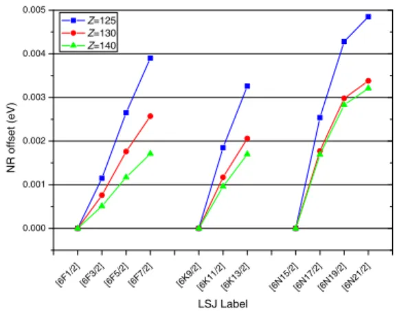
In order to assess the generality of this problem, we have investigated several other characteristic systems. El-ement 125, for example, is the first elEl-ement with a popu-lated 5gorbital [3,4]. We have calculated the NR offset for a configuration with 125 electrons [Rn]5f146d107s27p68s25g6f4 and Z = 125, 135 and 140. The results are presented on Fig. 2. We find three groups of levels with LSJ labels, four levels with label 6F
J (J = 1/2 toJ = 7/2), three levels with label 6K
J (J = 9/2 to J = 13/2) and four levels with label 6N
J (J=15/2 to J = 21/2). The NR offset in each group is of the order of a few meV, while the (non-relativistic) energy difference between the two first groups is 0.19 eV, and between the first and the last groups is around 0.25 eV. The figure also shows that the NR offset gets smaller when Z increases as expected.
Table 2.Total relativistic energy [Ener. (BSC)], including all-order Breit and QED corrections, total non-relativistic energy [ Ener. (NR)], and NR Offset for the ground configuration of uranium, relative to the 5f36d7s2 5L6 energy, which is the lowest level of the configuration. Correlation has not been in-cluded. One can observe a splitting in the NR energy between the 5H levels and the 5L levels, which should be exactly
de-generate. The fine-structure can be improved by subtract the NR offset from the relativistic energy.
Label Ener. (BSC) Ener. (NR) NR Offset
3P0 1.25373 1.22751
5D1 1.62153 1.22803
5G2 1.28675 0.89836
5H3 0.91680 0.70185 0.0251
5H4 1.05358 0.67678 0.0000
5K5 0.14628 0.01169
5L6 0.00000 0.00000 0.0000
5L7 0.42167 0.00181 0.0018
5L8 0.85283 0.00333 0.0033
5L9 1.28393 0.00284 0.0028
We have also investigated the lower excited states of a somewhat simpler system, element 118 (eka-radon). We have explored the [Rn]5f146d107s27p58swhich should ex-hibit no NR offset (it has single parent states) and [Rn]-5f146d107s27p57d. The results are presented on Table 3. As expected, the 7p58s3P
J states do not exhibit an NR offset, within our numerical accuracy. The 7p57d3L
J con-figurations however do have a strong NR offset, up to 0.8 eV, much larger than we expected from the other results presented above, and the largest ever observed. Clearly, such a large offset would render any calculation of the fine structure splitting of eka-radon useless, unless the results are corrected for the NR offset.
We would like to note that subtracting the NR offset is only a partial fix, since it was shown in Ref. [70] that not only the fine structure is affected, but also the level energy. The only possible solution are thus to do
calcu-[3P0] [5D1] [5G2] [5H3] [5H4] [5K5] [5L6] [5L7] [5L8] [5L9] 0.0
0.2 0.4 0.6 0.8 1.0 1.2 1.4 1.6 1.8
Energy (eV)
LSJ Label
BSC offset subtracted NR offset subtracted
Fig. 1. Non-relativistic offset on the ground configuration of uranium. “Ener. (BSC off. sub)”: total MCDF energy, with all QED corrections, using the full Breit operator in the SCF process, relative to the 5f36d7s2 5L6energy to which the non-relativistic offset has been subtracted. “Ener. (NR off. sub)”: Total non-relativistic energy, to which the non-relativistic off-set for members of the same LS multiplet has been subtracted, relative to the 5f36d7s2 5L6 energy. The two 5H
J and the four5LJ levels have thus identical non-relativistic energy as it should be. Uncorrected energy and NR offset are displayed in Table 2
[6F1 /2]
[6F3 /2]
[6F5 /2]
[6F7 /2]
[6K 9/2]
[6K 11/2
]
[6K 13/2
]
[6N 15/2
]
[6N 17/2
]
[6N 19/2
]
[6N 21/2
] 0.000
0.001 0.002 0.003 0.004 0.005
NR
offset
(eV
)
LSJ Label Z=125
Z=130 Z=140
Fig. 2. Non-relativistic offset for the6F
J,6KJ and 6NJ LS
configurations for the ground configuration of an atom with 125 electron.Z= 125, 130 and 1340 have been evaluated. This contribution should be negligible compared to correlation. For each LS group, the offset is evaluated by subtracting the lower energy of the group to the others.
Table 3. Non-relativistic offset on the lower excited config-urations of eka-radon (Z=118). For each member of a multi-plet, as, e.g., 7p57d3D, we evaluate the difference between the member with the lowest non-relativistic energy and the others. Non-relativistically, all member of a multiplet with identical LS labels should have an energy independent of the total angular momentumJ.
J 7p57d3D J 7p57d3F J 7p57d3P J 7p58s3P
1 0.801 2 0.335 0 0.000 0 0.000
2 0.000 3 0.000 1 0.002 1 0.002
3 0.336 4 0.000 2 0.802 2 0.002
limit in super-heavy elements and to correct for the non-relativistic offset, as it can be large in some cases.
3.2 Effect of the all-order Breit operator on simple systems
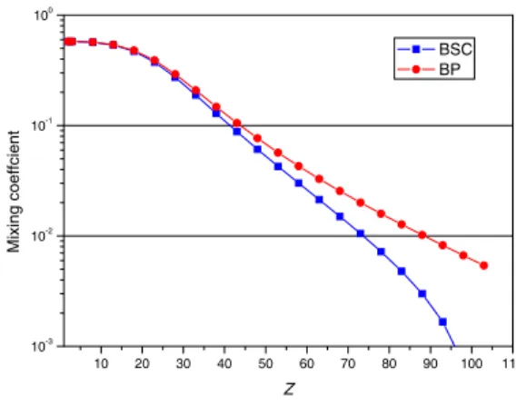
The use of different form of the electron-electron inter-action in the self-consistent field process has a profound qualitative influence on the behavior of variational cal-culations that goes beyond changes in energy. In partic-ular the mixing coefficients between configurations con-tributing to intermediate coupling are strongly affected (and thus the values of many operators would be like-wise affected). For example, let us examine the very sim-ple case of the 1s2p3P
1 state in two-electron system. In a MCDF calculation, intermediate coupling is taken care of by calculating |1s2p3P
1i=c1 | 1s2p1/2J = 1i+c2 | 1s2p3/2J = 1i. The evolution as a function of the atomic number Z of thec2 coefficient, is plotted on Fig. 3, with only the Coulomb interaction, or the full Breit interaction made self-consistent. The figure shows clearly that the in-clusion of the Breit interaction in the SCF process lead to values ofc2that are one order of magnitude lower at
high-Z that when only the Coulomb interaction is included. It means that the JJ coupling limit is reached much faster. This has some influence even in the convergence of the cal-culation: as the exchange potential for the 2p3/2orbital is proportional toc1
c2
2
, it becomes very large, and the cal-culation does not converge. This can be traced back to a negative energy continuum problem. If we use the method described in Ref. [26] to solve for the 2p3/2, then conver-gence can be reached, provided the projection operator that suppress coupling between positive and negative en-ergy solution of the Dirac equation is used. On Fig. 4, the different contributions to the 1s2p 3P
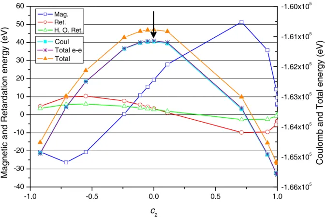
1 level energy are plotted at Z = 40. The minimum, which corresponds to the level energy, is obtained for a mixing coefficient (ha-bitually obtained by diagonalization of the Hamiltonian matrix), c2 = 0.104. The shape of the magnetic and re-tardation energy contribution, as observed on the figure, shows clearly that the curve used to find the minimum (which represents the sum of the contribution of the mean values of the operators in Eqs. (3a), Eqs. (3b), and (4)) is shifted to the left compared to the pure Coulomb con-tribution. This explain why the mixing coefficients gets
much smaller when using the Breit interaction in place of the Coulomb interaction in the SCF process. At high-Z
this lead to an extra difficulty to achieve convergence: as can be seen in Figs. 5 and 6, the minimum corresponding to the 1s2p 3P
1 state (the one lower in energy) is very close to c2 = 0. It thus sometimes happens during the convergence, thatc2 changes sign, leading to very tedious tuning of the convergence process. This is even worse for the 1s2p 1P
1 state, because one is trying to reach the maximum energy. In that case the oscillation of thec1 co-efficient around zero are impossible to damp. Obviously, such problems will slowly disappear when going to neutral systems. For example, in neutral nobelium (Z = 102) c2 changes only from 0.47250012 to 0.47316712.
10 20 30 40 50 60 70 80 90 100 110
10-3
10-2
10-1
100
M
ix
in
g
c
o
e
ff
c
ie
n
t
Z
BSC BP
Fig. 3. Variation with Z of mixing c2 coefficient for the 1s2p3P1 level of helium-like ions. BP: Only the Coulomb
teraction is used in the SCF process. BSC: The full Breit in-teraction is used in the SCF process
4 Relativistic and QED effects on transition
energies and probabilities
4.1 Beryllium isoectronic sequence correlation
It is interesting to investigate simple many-body system, that can be calculated accurately, to see which kind of highly relativistic effects can be expected in the limitZα→ 1. In that sense the beryllium isoelectronic sequence is an interesting model case, as it exhibit a very strong intrashell coupling between the 1s22s2J = 0 and 1s22p2
-1.0 -0.5 0.0 0.5 1.0 -2
-1 0 1 2 3 4 5
-2.760x10⁴
-2.758x10⁴
-2.756x10⁴
-2.754x10⁴
-2.752x10⁴
-2.750x10⁴
-2.748x10⁴
-2.746x10⁴
-2.744x10⁴
-2.742x10⁴
Magnetic and Retardation energy (eV)
c
2Mag. Ret. H. O. Ret.
Coul Total e-e Total
Coulomb and Total energy (eV)
Fig. 4. Variation of the different contributions to the energy as a function of the mixing coefficientc2, for the 1s2p3P1 level
at Z = 40. The arrow indicates the position of the 1s2p3P1 energy, at the minimum aroundc2 = 0.104. Left axis:“Mag.”:
Magnetic energy, Eq. (3b). “Ret.”: Breit retardation, Eq. (4). “H.O. Ret.”: higher-order retardation. Right axis:“Coul.”: Coulomb energy Eq. (3a). “Total e-e”: sum of the 4 preceding contributions. “ Total”: total level energy including all QED corrections.
in Fig. 7. One can see that the ground state, which is 1s22s2J = 0 at lower Z, becomes 1s22p21/2J = 0. This can be seen on the mixing coefficients as plotted on Fig. 7. This translates into a strong increase in the loop-after-loop vacuum polarization contribution. Obviously, if we were able to evaluate other second-order QED calcula-tion than loop-after-loop vacuum polarizacalcula-tion, including off-diagonal two-electron self-energy matrix elements for quasi-degenerate state, following recent work on helium-like systems [71,72,73], there could be more unexpected effects to observe.
While not displaying such a feature, the total corre-lation energy increases strongly, reaching up to 3.6 keV. One can observe effects on other properties of the atom, like orbital energies and mean orbital radius. Figure 8 shows that, in the same atomic number range when the ground state changes of structure, the 2p3/2orbital radius and energy exhibit a very strong change. The behavior of the ground state must be connected to the fact that the small component of 2p1/2 orbitals, as can be seen from
Eq. (7), has a s behavior, and the ratio between small and large component is of order Zα. It is thus under-standable that such effects could occurs whenZα→1. It should be noted that this effects happens even with a pure Coulomb electron-electron interaction, which is one more proof it is only connected with the behavior of the one-electron wavefunctions. We investigated the similar case of the magnesiumlike sequence, which exhibit strong in-trashell coupling between the 3s, 3pand 3dorbitals, but we could not observe any effect on energies in this range of Z. However the [Ne]3p2
1/2 mixing coefficient started to increase faster aroundZ= 128, but convergence problems prohibited us to investigate higherZ.
4.2 Relativistic correlations on the neon isoelectronic sequence
-1.0 -0.5 0.0 0.5 1.0 -40
-30 -20 -10 0 10 20 30 40 50 60
-1.66x10⁵
-1.65x10⁵
-1.64x10⁵
-1.63x10⁵
-1.62x10⁵
-1.61x10⁵
-1.60x10⁵
Magnetic and Retardation energy (eV)
c
2 Mag.Ret. H. O. Ret.
Coul Total e-e Total
Coulomb and Total energy (eV)
Fig. 5. Variation of the different contributions to the energy as a function of the mixing coefficientc2, for the 1s2p3P1 level
at Z = 92. The arrow indicates the position of the 1s2p3P1 energy, at the minimum aroundc2 = 0.002. Left axis:“Mag.”:
Magnetic energy, Eq. (3b). “Ret.”: Breit retardation, Eq. (4). “H.O. Ret.”: higher-order retardation. Right axis:“Coul.”: Coulomb energy Eq. (3a). “Total e-e”: sum of the 4 preceding contributions. “ Total”: total level energy including all QED corrections.
electrons are a small enough system that can be calcu-lated with rather large basis sets. We have extended the calculation performed in Ref. [7] to superheavy elements (Z = 134). All 10 electrons are excited to all virtual or-bitals up to a maximumnℓ, that is varied from 3dto 6h. The results are presented in Table 4 and plotted on Fig. 9. The trend found up toZ= 94 in Ref. [7] extend smoothly to largerZ, but is enhanced. The total correlation energy becomes very large. It doubles when going from Z = 95 to Z = 134, the highest Z for which convergence could be reached. The speed of convergence as a function ofnℓ
does not change with increasingZ.
4.3 Transition energies and probabilities in nobelium and element 118 (eka-radon)
In this section we study the different contributions to the energy and transition probabilities of nobelium (Z= 102) and eka-radon (Z= 118). Nobelium is the next candidate for measurement of its first excited levels transition
en-Table 4. Total correlation energy for neonlike ions, with the Breit interaction included in the SCF, as a function of the most excited orbital included in the basis set.
Z all→3d all→4f all→5g all→6h
-1.0 -0.5 0.0 0.5 1.0 -40
-30 -20 -10 0 10 20 30 40 50 60
-1.66x10⁵
-1.65x10⁵
-1.64x10⁵
-1.63x10⁵
-1.62x10⁵
-1.61x10⁵
-1.60x10⁵
Magnetic and Retardation energy (eV)
c
2 Mag.Ret. H. O. Ret.
Coul Total e-e Total
Coulomb and Total energy (eV)
Fig. 6. Variation of the different contributions to the energy as a function of the mixing coefficientc1, for the 1s2p1P1 level
atZ = 92. The arrow indicates the position of the 1s2p1P1 energy, at themaximum around c1 = 0.002. Left axis:“Mag.”:
Magnetic energy, Eq. (3b). “Ret.”: Breit retardation, Eq. (4). “H.O. Ret.”: higher-order retardation. Right axis:“Coul.”: Coulomb energy Eq. (3a). “Total e-e”: sum of the 4 preceding contributions. “ Total”: total level energy including all QED corrections.
ergy by laser spectroscopy. Large scale calculations have been performed recently [21]. Here we examine a number of corrections not considered in Ref. [21]. For the 7s2 1S
0 ground state, we did a MCDF calculation taking into ac-count all single and double excitations, except the one corresponding to the Brillouin theorem, from the 5f and 7sshells to the 7p, and 6dshells (48 jj configurations). For the excited states we included excitations from 5f, 7sand 7pshells to the 7pand 6dones. This leads to 671 jj con-figurations for the 7s7p3P
1 and 7s7p1P1 states and 981 for 7s7p3P2. The results of this calculation are presented on Table 5 for the transition energies and on Table 6 for transition probabilities. It is clear from these two tables that many contributions that are important for level en-ergies are completely negligible for transition probabilities in this case. This is not true for highly charged ions, even at much lowerZ. In particular two-loop QED corrections, even though many of them have not been calculated from
n > 2, should remain completely negligible, since they will be of the same order of magnitude as the
loop-after-loop and K¨all`en and Sabry contributions. The self-energy screening is almost exactly compensating the self-energy, but leaves a contribution that should be visible if one can calculate correlation well enough. At the present level of accuracy, calculation of the pure Coulomb correlation is the real challenge as it requires considerable effort on the size of configuration space.
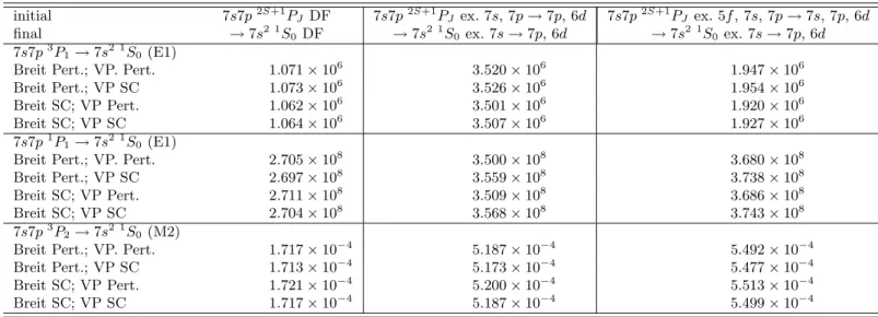
The transition probabilities on Table 6 have been eval-uated with different approximation, using theoretical en-ergies. Here the choice of the wavefunction optimization technique has a sizeable effect. It remains small compared to correlation, but still at the level of 0.2%. We also inves-tigated the effect of using fully relaxed orbitals on both initial and final state. In particular we checked at the Dirac-Fock level of approximation, what is the order of magnitude of taking into account non-orthogonality be-tween initial and final state orbitals. We found 2.2% for the 3P
1 → 1S0 transition, 0.014% for the 1P1 → 1S0 transition and -0.025% for the 3P
im-80 90 100 110 120 130 10-1
100
101
102
103
104
0.0 0.1 0.2 0.3 0.4 0.5 0.6 0.7 0.8 0.9 1.0
E
(eV)
Z L-a-L Uelhing
Correlation
c
2 i
c 1
2
c 3
2
c 3
2
Fig. 7.Loop-after-loop Uehling contribution to berylliumlike ions ground state energy (changed of sign), obtained by includ-ing the Uehlinclud-ing potential in the SCF. The intrashell correlation energy is also plotted (left axis), as well as the square of the mixing coefficients of the 1s22s2J = 0, 1s22p21/2J = 0 and
1s22p23/2J= 0 configurations (right axis).
80 90 100 110 120 130 140
0.0 5.0x10⁴ 1.0x10⁵ 1.5x10⁵ 2.0x10⁵ 2.5x10⁵ 3.0x10⁵ 3.5x10⁵ 4.0x10⁵
0.00 0.01 0.02 0.03 0.04 0.05
Orbital energy (eV)
c 2
OE(1s) OE(2s) OE(2p1/2)
OE(2p3/2) r(1s)
r(2s) r(2p1/2) r(2p3/2)
O
rbit
al radii (a.
u.
)
Fig. 8.Orbital radii (right axis) and one-electron energies (left axis) for Be-like ions
portant to evaluate the matrix elements for off-diagonal operators, taking account non-orthogonalities between ini-tial and final state orbitals, as it can change dramatically the contribution of a given CSF, since overlaps between correlations orbitals in initial and final states can be very different from either one or zero.
As another example we have also calculated several transition energies and rates for element 118, which are displayed in Table 7. For the most intense 7p57d→7s27p6 transitions and for the 7p58s→7s27p6transitions we did a MCDF calculation, taking into account all single and double excitations, (except the ones corresponding to the Brillouin theorem) from the 7sand 7pshells to the 7dand 6fshells for the 7p6 1S
0ground state (38 jj configurations) and for the 7p57d excited states (657 jj configurations),
10 20 30 40 50 60 70 80 90 100 110 120 130 140
-55 -50 -45 -40 -35 -30 -25 -20 -15 -10 -5
Correlation energy (eV)
Z
all -> 3d all -> 4f all -> 5g all -> 6h
Fig. 9. Total correlation energy for neonlike ions, with the Breit interaction included in the SCF, as a function of the most excited orbital included in the basis set.
and from the 7pand 8sshells to the 7dand 6f shells for the 7p58sexcited states (151 jj configurations).
The transition energy was calculated for some of these transitions, with and without including the vacuum polar-ization and Breit interaction in the SCF process, and we concluded that the transition energy is not significantly affected by the inclusion of these interactions in the SCF. This is illustrated on Fig. 10 that shows the transition energy values for 7p57d3P
1transition.
6.81450 6.81455 6.81460 6.81465 6.81470 6.81475 6.81480 6.81485 6.81490
Transition energy (eV)
BSC, VPSC BSC, VPP BP, VPP
Table 5. Transition energies for the lower energy levels of nobelium (eV). Coul.: DF Coulomb energy. Mag. (pert), Ret. (pert.), Higher order ret. (pert.): Contribution of the Magnetic, Breit retardation and higher-order retardation in first order of perturbation. All order Breit: effect of including the full Breit interaction in the SCF. Coul. Corr.: Coulomb correlation. Breit Corr.:Contribution of all Breit terms to the correlation energy. Self-energy (FS): self-energy and finite size correction. Self-energy screening: Welton approximation to self-energy screening. Vac. Pol. (Uehling): mean value of the Uehling potential (order α(Zα)). VP (muons, Uehling): vacuum polarization due to muon loops. VP Wichman and Kroll: correction to the Uehling potential (orderα(Zα)3). Loop-after-loop V11: iterated Uehling contribution to all orders. VP (K¨all`en et Sabry): two-loop contributions to vacuum polarization. Other 2nd order QED: sum of two-two-loop QED corrections not accounted for in the two previous one. Recoil: sum of lowest order recoil corrections (see, e.g., [74]). The number of digits presented in the table is not physically significant, but is necessary to show the size of some contributions. The physical accuracy is not better than 1 digits.
Contribution 3P1→ 1S0 1P1→ 1S0 3P2→ 1S0
Coul. 1.69909 3.20051 2.19931
Mag. (pert) 0.00070 −0.00420 −0.00347
Ret. (pert.) −0.00048 0.00005 −0.00058
Higher order ret. (pert.) −0.00119 0.05048 −0.00231 All order Breit (pert) 0.00002 −0.05877 0.00003
Coul. Corr. 0.59560 0.60414 0.55545
Breit Corr. −0.00208 −0.00229 −0.00194
Self-energy (FS) −1.60884 −1.72025 −1.76085 Self-energy screening 1.59030 1.72940 1.74228
Vac. Pol. (Uehling) 0.00610 0.00435 0.00648
VP (muons. Uehling) 0.00000 0.00000 0.00000
VP Wichman and Kroll −0.00030 −0.00019 −0.00033 Loop-after-loop Uehl. 0.00002 0.00012 0.00003 VP (K¨all`en and Sabry) 0.00004 0.00002 0.00005
Other 2nd order QED 0.00000 0.00000 0.00000
Recoil −0.00082 −0.00081 −0.00082
Total 2.28 3.80 2.73
Ref. [21] II 2.34 3.49
Ref. [21] I 2.60 3.36
Table 6. Effect of correlation, Breit interaction and all order vacuum polarization on transition probabilities of nobelium. DF: Dirac-Fock. VP: vacuum polarization. ex.: excitation
initial 7s7p2S+1P
J DF 7s7p2S+1PJ ex. 7s, 7p→7p, 6d 7s7p2S+1PJ ex. 5f, 7s, 7p→7s, 7p, 6d
final →7s2 1S0 DF →7s2 1S0 ex. 7s→7p, 6d →7s2 1S0 ex. 7s→7p, 6d
7s7p3P1→7s2 1S0 (E1)
Breit Pert.; VP. Pert. 1.071×10⁶ 3.520×10⁶ 1.947×10⁶
Breit Pert.; VP SC 1.073×10⁶ 3.526×10⁶ 1.954×10⁶
Breit SC; VP Pert. 1.062×10⁶ 3.501×10⁶ 1.920×10⁶
Breit SC; VP SC 1.064×10⁶ 3.507×10⁶ 1.927×10⁶
7s7p1P1→7s2 1S0 (E1)
Breit Pert.; VP. Pert. 2.705×10⁸ 3.500×10⁸ 3.680×10⁸
Breit Pert.; VP SC 2.697×10⁸ 3.559×10⁸ 3.738×10⁸
Breit SC; VP Pert. 2.711×10⁸ 3.509×10⁸ 3.686×10⁸
Breit SC; VP SC 2.704×10⁸ 3.568×10⁸ 3.743×10⁸
7s7p3P2→7s2 1S0 (M2)
Breit Pert.; VP. Pert. 1.717×10⁻⁴ 5.187×10⁻⁴ 5.492×10⁻⁴
Breit Pert.; VP SC 1.713×10⁻⁴ 5.173×10⁻⁴ 5.477×10⁻⁴
Breit SC; VP Pert. 1.721×10⁻⁴ 5.200×10⁻⁴ 5.513×10⁻⁴
Table 7. Transition energies and transition rates to the ground state 5f156d107s27p6 1S0 of eka-radon (element 118). The transition values from states labeled withc were calculated with correlation up to 6f, as well as the ground state.
Initial State Transition Energy Transition Rate
(eV) (s−1)
5f15 6d107s2 7p5 7d 3D1+3P1 c 10.43 9.86×10⁸
3P1 c 6.81 5.53×10⁷ 3D1+1P1 c 7.2 9.98×10⁶
3P2 6.08 1.41
×10−2
3F2 16.95 1.11×10⁻²
3F3 6.15 1.30×10⁻³
1D2 6.25 1.10×10⁻³
3D3 6.22 7.52
×10−4
3F4 6.01 3.91×10⁻¹⁴
3P0 c 6.64
5f156d107s27p5 8s 1P1 c 4.73 2.04×10⁸
3P2 c 4.3 2.04
×10−3
5 Relativistic and QED effects on Land´
e
factors, atomic radii and electronic densities
Although transition energies and probabilities, as well as ionization potential, are important quantities, it is in-teresting to study relativistic and QED effects on other atomic parameters, like Land´eg-factors, atomic radii and electronic densities. Land´e factors, which define the strength of the coupling of an atom to a magnetic field, can help characterize a level.
In some experiments concerning superheavy elements, singly ionized atoms are drifted in a gas cell, under the in-fluence of an electric field. The drift speed can be related, in first approximation, to the charge distribution radius of the ion [75,76]. In this context, it can also be interesting to look at the atomic density, and see how it is affected by relativistic and QED effects. In that case, though, we can only get a feeling of this effect by comparing den-sities calculated with and without the Breit interaction self-consistent, or with and without the Uehling potential included in the differential equation. There is currently no formalism that would enable to account for changes in the wavefunction related to the self-energy.
We define the radial electronic density as
r2ρ(r) = Z
dΩr2ρ(r, Ω)
= X
i∈occ.orb.
̟i
Pi(r)2+Qi(r)2
, (10)
whereP andQare defined in Eq. (7), and the̟iare the orbital effective occupation numbers,
̟i= X
j
c2jnij, (11)
where the sum extend over all configuration containing orbital i, and nij is the occupation number of this or-bital in the configurationj. The density is normalized to R∞
0 drr
2ρ(r) =Ne, where N
e is the number of electrons in the atom or ion.
The effect of the Breit interaction and vacuum polar-ization on the charge density of the ground state of Fm+ ([Rn]5f126s) is shown on Fig. 11. The inclusion of both contributions leads to local changes of around 1% in the charge density. It is rather unexpected that both contri-bution extend their effects way pass their range, in par-ticular for the vacuum polarization potential, which has a very small contribution forr >1/α= 0.0073 a.u.
10-4 10-3
10-2 10-1
100 101 10-4
10-3 10-2 10-1 100 101 102 103
U
r
2 (
a
.u
)
r (a.u.)
Density Diff (Bsc) Diff (Vsc) <r> msr Rmax(7s)
Fig. 11. Total electronic density of Fm+. The vertical lines
represents, from left to right the mean radius, the mean spher-ical radius (“rms”) and the mean radius of the outermost or-bital (7s). “Density”: total electronic density Eq. (10). “Diff (Bsc)”: absolute value of the variation in the density due to the inclusion of the Breit interaction in the SCF. “Diff (Vsc)”: absolute value of the variation in the density due to the in-clusion of the Uehling potential in the differential equations (NB: the dip in the curve correspond to sign changes of the correction).
correlation between the value of the maximum charge den-sity of the outermost core electron shell and the ionic ra-dius of an atom [77]. Such a definition, however, does not provide a way to take into account mixing of outer shell in MCDF calculations. Other authors have chosen either the mean radius of a specific orbital hrn,l,ji [78] or weighted mean radius [79]. Results have been obtained for bohrium and hassium. It is not at all obvious either than what is true in crystals must be valid for singly charged ions drift-ing in a gas. Here we have evaluated four different quan-tities and their dependence in the Breit interaction and vacuum polarization. We have evaluated the position of the maximum density of the outermost orbital, the mean radius of the outermost orbitalhrn,l,ji, the atom mean ra-dius, and the atom mean spherical radius. The two first quantities have been tested in detail, but they cannot rep-resent the ionic radius when one has a complex outer shell structure or when one calculate correlation. The mean ra-dius of the atom is represented as
hr(p)at.i= 1
Ne Z ∞
0
drrpr2ρ(r)
= 1
Ne X
i∈occ.orb.
̟ihr(p)ni,li,jii (12)
for p = 1, and the mean spherical radius is obtained as q
hr(2)at.i. Both can be calculated in a MCDF model, as the
̟i contain both the occupation numbers and the mixing coefficients. As an example, we have plotted the contri-bution to hrat.(p)i to Sg+ on Fig. 12 of individual values of ̟ihr(p)ni,li,jii for the different orbitals. Contrary to the
individual orbitals quantities or to the average performed only on the outer shell, like in Ref. [9], both quantities have sizeable contributions from several outer shells. The 7s, 6p, 5fand 6dcontribute significantly to both the mean and the mean spherical atomic radius, but the contribu-tion of the 6d orbitals is more dominant for the mean spherical radius. The results for singly charged ions with 57≤Z≤71 and 90≤Z≤108 are presented on Table 8 and plotted on Fig. 13. The comparison between mean ra-dius and mean spherical rara-dius with the Breit interaction in the SCF process with Coulomb values, shows changes around 0.04% to 0.08% depending on the atomic number. Self-consistent vacuum polarization has an effect 2 to 4 times smaller, depending on the element. We emphasize the fact that we used for the ion the configuration corre-sponding to the ground state of a Dirac-Fock calculation (i.e., without correlation), as given in [6]. For a few ele-ments, the physical ground state configuration, as given for example on the NIST database, is different.
We have used the definition above to evaluate the effect of correlation on the ion radii. The calculation has been performed on neutral nobelium (Z= 102). The results are presented on Table 9. One can see that the radius of max-imum density follows exactly the trend of the mean radius of the outer orbital. However the atomic mean radius and mean spherical radius follow a different trend.
There has been two experiments measuring drift time of singly ionized transuranic elements in gases. One
mea-sured the relative velocity of Am+with respect to Pu+[75] and an other one measured the same quantity for Cf+and Fm+ [18]. The results of these experiments are expressed as
∆rA−B =
rA−rB
rB
. (13)
The experiments above provide∆rAm+
−Pu+=-3.1±1.3%
and∆rFm+−Cf+=-2% respectively, which shows a
shrink-age of Am as compares to Pu and of Fm as compared to Cf. The comparison between these experiments and the calculation of singly charged ion radii from Table 8 is shown in Table 10. Although it is difficult to draw any firm conclusion from so few data, it seems that
q
hrat.(2)i re-produces best the experiment, followed byhrat.(1)i. We want to point out that the< r7s>values for neutral atom, from Ref. [5], or ours, which are in good agreement gives a -1.5% change for Am/Pu and -3.0% for Fm/Cf, compare well with experiment. The 7sradius of the singly charged ions, as shown in Table 8, increases when going from Am to Pu, thus leading to a ratio of the wrong sign, while the 5f average radius, or the global atomic radii as defined here all show the right trend. The change of behavior for Am, is due to the relative diminution of the l(l+ 1)/r2 barrier compared to the Coulomb potential as a function ofZ. The 5f radius reduces then strongly, leading to the change of the structure of the ground configuration, and to the change of the radius of the 7sorbital.
1s 2s 3s4s 5s 6s 7s2p*3p*4p*5p*6p*2p 3p 4p 5p 6p3d*4d*5d*6d* 3d 4d 5d 6d4f*5f* 4f 5f
To tal
0.0 0.1 0.2 0.3 0.4 0.5 0.6 0.7 0.8 0.9
<r>×occupation / Ne (a.u.)
Orbital label <r>
<r2>
Fig. 12. Contribution to the mean radius hrat(p.)i to Sg+ of individual values of ̟ihr(npi),li,jii for the different orbitals and
p= 1 and 2, together with the total values on the right. Stared orbital labels correspond to the orbital withj=l−1
2.
Table 8.Singly ionized atom radii (a.u.) for lanthanide 57≤Z ≤71 and actinide and transactinide 90≤Z≤108
Z Config. Label < r > √< r2> outer orb.
lab. Rmax <4f5/2> <4f7/2> <5d3/2> <5d7/2> <6s1/2>
57 5d2 3F
2 0,6903 1,0365 5d 2,2820 2,8629 2,8900
58 4f5d2 4H
7/2 0,6789 1,0121 5d 2,2005 1,0862 1,1033 2,7568 2,7949
59 4f36s 5I
4 0,6750 1,0458 6s 3,8004 1,0589 1,0667 4,2924
60 4f46s 6I
7/2 0,6646 1,0256 6s 3,7359 1,0054 1,0190 4,2252
61 4f56s 7H
2 0,6544 1,0062 6s 3,6741 0,9624 0,9796 4,1608
62 4f66s 8F
1/2 0,6442 0,9874 6s 3,6171 0,9249 0,9392 4,1012
63 4f76s 9S
4 0,6342 0,9692 6s 3,5627 0,8920 0,8999 4,0438
64 4f75d6s 10D
5/2 0,6357 0,9708 6s 3,3408 0,8218 0,8221 2,4547 2,4846 3,7930
65 4f96s 7H
8 0,6162 0,9373 6s 3,4711 0,8502 0,8541 3,9568
66 4f106s 6I
17/2 0,6074 0,9219 6s 3,4289 0,8254 0,8345 3,9163
67 4f116s 5I
8 0,5987 0,9070 6s 3,3871 0,8022 0,8165 3,8758
68 4f126s 4H
13/2 0,5903 0,8926 6s 3,3464 0,7804 0,7995 3,8359
69 4f136s 3F
4 0,5820 0,8786 6s 3,3070 0,7605 0,7811 3,7976
70 4f146s 2S
1/2 0,5739 0,8649 6s 3,2699 0,7430 0,7613 3,7611
71 4f146s2 1S
0 0,5876 0,9133 6s 2,9761 0,6922 0,7057 3,4229
<5f5/2> <5f7/2> <6d3/2> <6d7/2> <7s1/2>
90 5f26d 4K
11/2 0.5873 0.9117 6d 2.5751 1.96004 1.95812 3.16141 3.18613
91 5f26d7s 5K
5 0.5977 0.9521 7s 3.5491 1.54181 1.57544 2.85704 2.9741 3.99617
92 5f36d7s 6L
11/2 0.5926 0.9377 7s 3.4779 1.42706 1.44552 2.78857 2.86351 3.92351
93 5f46d7s 7L
5 0.5873 0.9239 7s 3.4116 1.3478 1.36699 2.72666 2.79424 3.85537
94 5f56d7s 8K
7/2 0.5821 0.9107 7s 3.3498 1.28511 1.30541 2.67874 2.73928 3.7917
95 5f77s 9S
4 0.5699 0.8822 7s 3.4279 1.27013 1.29869 3.8992
96 5f77s2 8S
7/2 0.5805 0.9217 7s 3.2104 1.16578 1.18716 3.65864
97 5f86d7s 9G
7 0.5670 0.8761 7s 3.1840 1.14449 1.16614 2.62581 2.688 3.62195
98 5f107s 6I
17/2 0.5553 0.8493 7s 3.2905 1.14462 1.18171 3.77066
99 5f117s 5I
8 0.5503 0.8385 7s 3.2461 1.10705 1.14777 3.72772
100 5f127s 2H
11/2 0.5456 0.8293 7s 3.2294 1.07281 1.11537 3.72114
101 5f137s 3F
4 0.5403 0.8174 7s 3.1625 1.0417 1.08491 3.64662
102 5f147s 2S
1/2 0.5353 0.8071 7s 3.1235 1.01352 1.05406 3.6087
103 5f147s2 1S
0 0.5435 0.8385 7s 2.8837 0.95846 0.990419 3.32578
104 5f146d7s2 2D
3/2 0.5441 0.8392 7s 2.7464 0.917421 0.941578 2.33571 3.16377
105 5f146d27s2 3F
2 0.5436 0.8355 7s 2.6309 0.881333 0.900734 2.17264 2.25313 3.02942
106 5f146d47s 6D
1/2 0.5376 0.8127 7s 2.5150 0.850008 0.867203 2.11798 2.21807 2.87277
107 5f146d47s2 5D
0 0.5409 0.8240 7s 2.4351 0.820103 0.834045 1.95902 2.01018 2.80344
108 5f146d57s2 6S
5/2 0.5396 0.8183 7s 2.3426 0.790744 0.807474 1.86004 1.95516 2.69468
Table 9.Correlation effects on the mean radius and mean spherical radius of No.
< r >(a.u.) var. √< r2>(a.u.) var.
Ra5f147s2 1S0 0.574391 0.932605
+ excit. of 7s→7p, 6d 0.573724 -0.12% 0.928191 -0.47%
+ excit. of 7s, 5f→7p, 6d 0.573309 -0.19% 0.925313 -0.78%
Table 10.Comparison between different definition of the ionic radii and experiment. We define the average radius of 5f or-bitals as< r5¯ f >= (6< r5f5/2>+8< r5f7/2>)/14
Exp. Theo.
∆rAm+
−Pu+[75] -3.1% (±1.3%) < rAt.> -2.1%
p
< r2
At.> -3.1% ¯
< r5f > -0.8%
< r7s> 2.8%
∆rFm+
−Cf+ [18] -2.0% < rAt.> -1.7%
p
< r2
At.> -2.4% ¯
< r5f > -5.9%
< r7s> -1.3%
85,86,87,88,89]. To our knowledge, there has been only one calculation dealing with QED corrections in heavy
elements, in which the Feynman diagrams correspond-ing to self-energy and other corrections were evaluated. This calculation concerned alkali elements up to francium (Z = 87) [90]. Here we deal with much more complex system, with several open shells, and we calculate QED corrections due to the inclusion of the Breit interaction and of the vacuum polarization in the SCF, as well as the contribution from the electron anomalous moment. The coupling of an atom with a magnetic moment µto a ho-mogeneous magnetic fieldB gives an energy change
∆E=−µ·B (14)
whereµ=−gJµBJ,gJbeing the Land´e factor andµBthe Bohr magneton. The anomalous electron magnetic mo-ment corrections can be written (see, e.g., [91] and refer-ence therein) as
∆gJ= (g−2)
hJ||βΣ||Ji
p
50 60 70 80 90 100 110 2.0
2.5 3.0 3.5 4.0 4.5
0.5 0.6 0.7 0.8 0.9 1.0 1.1
Radius of outermost orbital (a.u.)
Z
Rmax rout
<r> <r2 >1/2
<
r
> and <
r
2>
1
/2 (a
.u
.)
Fig. 13. Variation of< r >,√< r2> (right scale), of the
radius of the outermost orbital< rout>and of the maximum of the charge density of the outer orbital (Rmax. dens.) (left scaleas a function of the atomic numberZ.
Table 13.Correlation effect on the Land´eg-factor of the first excited states of nobelium.
Level 7s7p3P1 7s7p1P1 7s7p3P2
DF 1.49073 1.00932 1.50111
7, 7pexc.→7p, 6d 1.47691 1.02829 1.50027 7, 7p, 5fexc. →7p, 6d 1.48845 1.01507 1.50080
where g = 2 1 + α π+· · ·
is the electron magnetic mo-ment, β and Σ are 4×4 matrices, β =
I0 0I
and
Σ =
σ 0
0 σ
where I is a 2×2 identity matrix and σ
are Pauli matrices.
As an example, we illustrate the different effects by evaluating the Land´eg-factors for the ground configura-tion of neutral actinide and transactinide up toZ = 106, and of singly ionized lanthanide, actinide and transac-tinide up toZ = 106. The results are displayed on Table 11 for neutral atoms and on Table 12, for singly ionized atoms. The ground configuration of neutral atom comes from [92]. For singly ionized atoms, it has been taken from Refs. [6] for Z up to 106 and from [9] forZ = 107 and 108. Depending on the outer shell structures, the QED corrections can be dominated by either theg−2 correc-tion or the Breit correccorrec-tion (order of 0.1% of the Land´e factor). The vacuum polarization correction is at best one order of magnitude smaller atZ= 106.
In Table 13, we present correlation effects on the Land´e
g-factor of the lowest levels of No, evaluated with the same wavefunctions as in Sec. 4.3, with the Breit operator in the SCF process. The effect of correlation ranges from 0.6% to 0.02% depending on the level.
6 Conclusions
In this work we have evaluated the effects of self-consistent Breit interaction and vacuum polarization on level ener-gies, transition energies and probabilities Land´eg-factors on super-heavy elements. We have also studied their ef-fect on orbitals and atomic charge distribution radii and found very large effects on highly charged ions. We have found some hints, when studying Be-like ions, of rather strong non-perturbative correlation effects for Z ≈ 128. For neutral or quasi-neutral systems, self-consistent Breit interaction and vacuum polarization have a small but no-ticeable effects on Land´e factor and transition rates, which could be felt experimentally. Transition energies, on the other hand, are heavily dominated by Coulomb correla-tion. This is rather good news, since treating the Breit interaction self-consistently obliges to evaluate magnetic and retardation integrals during the SCF process, which are about one order of magnitude more numerous than Coulomb ones, leading to calculations that cannot fit on even on the largest computers available today, even with relatively small configuration space.
We have shown that very large non-relativistic offset may affect the fine structure separation of elements with several open shells. This should be carefully taken into account to avoid providing completely wrong results with all-order methods. We have also shown that the inclusion of the Breit interaction in the SCF process, because it get mixing coefficients closer to the jj limit, can noticeably complicate numerical convergence.
Acknowledgments
Laboratoire Kastler Brossel is Unit´e Mixte de Recherche du CNRS n◦C8552. This research was partially supported
by the FCT projects POCTI/FAT/44279/2002 and POCTI-/0303/2003 (Portugal), financed by the European Com-munity Fund FEDER, and by the French-Portuguese col-laboration (PESSOA Program, Contract n◦ 10721NF).
One of us (P.I.) thanks M. Sewtz for several discussions on this subject. The 8-processors workstation used for the cal-culations has been provided by an “infrastructure” grant from the “Minist`ere de La Recherche et de l’Enseignement Sup´erieur”.
References
1. Y.T. Oganessian, V.K. Utyonkov, V.L. Yu, F.S. Abdullin, A.N. Polyakov, R.N. Sagaidak, I.V. Shirokovsky, S.T. Yu, A.A. Voinov, G.G. Gulbekian et al., Phys. Rev. C 74(4), 044602 (2006)
2. S. Hofmann, G. M¨unzenberg, Rev. Mod. Phys.72(3), 733 (2000)
3. J.B. Mann, J.T. Waber, J. Chem. Phys.53(6), 2397 (1970) 4. B. Fricke, J.T. Waber, Actinides Reviews1(5), 433 (1971) 5. J.P. Desclaux, Atomic Data and Nuclear Data Tables
Table 11.QED [Eq. (15)], Breit and Uehling corrections on Land´eg-factors of neutral atoms with 90≤Z≤106
Z Conf. Label Land´e (Coul.) QED corr. Breit contr. Uehl. corr. Total
90 6d27s2 3F2 0.68158912 -0.00073903 -0.00031059 -0.00002136 0.68051814
91 5f26d7s2 4K
11/2 0.81847964 -0.00042068 -0.00020095 -0.00001531 0.81784271
92 5f36d7s2 5L6 0.73962784 -0.00060501 -0.00090733 -0.00001069 0.73810480 93 5f46d7s2 6L
11/2 0.63735126 -0.00084251 -0.00108525 -0.00000780 0.63541570
94 5f67s2 7F0
95 5f77s2 8S7/2 1.96702591 0.00224893 0.00193804 0.00000967 1.97122254
96 5f76d7s2 9D2 2.60336698 0.00372915 0.00336317 0.00002669 2.61048600 97 5f97s2 6H
15/2 1.29988703 0.00070147 0.00177562 0.00000642 1.30237054
98 5f107s2 5I8 1.22357731 0.00052300 0.00108516 0.00000375 1.22518921
99 5f117s2 4I15/2 1.18834647 0.00043997 0.00047015 0.00000159 1.18925817
100 5f127s2 3H6 1.16189476 0.00037811 0.00019838 0.00000062 1.16247187
101 5f137s2 2F
7/2 1.14180915 0.00033132 0.00005605 0.00000020 1.14219672
102 5f147s2 1S0
103 5f147s27p 2P1
/2 0.66661695 -0.00077309 0.00003007 0.00000003 0.66587396
104 5f146d27s2 3P0
104 5f147s27p2 3F2 0.69055158 -0.00071837 -0.00035975 -0.00006392 0.68940954 105 5f146d37s2 4F3/2 0.45467514 -0.00126763 -0.00122595 -0.00016406 0.45201750
106 5f146d47s2 5D0
6. G.C. Rodrigues, P. Indelicato, J.P. Santos, P. Patt´e, F. Parente, Atomic Data and Nuclear Data Tables86(2), 117 (2004)
7. J.P. Santos, G.C. Rodrigues, J.P. Marques, F. Parente, J.P. Desclaux, P. Indelicato, Eur. Phys. J. D37(2), 201 (2006) 8. N. Gaston, P. Schwerdtfeger, W. Nazarewicz, Phys. Rev.
A66(6), 062505 (2002)
9. E. Johnson, B. Fricke, T. Jacob, C.Z. Dong, S. Fritzsche, V. Pershina, J. Chem. Phys.116(5), 1862 (2002)
10. E. Eliav, U. Kaldor, Y. Ishikawa, Phys. Rev. Lett.74(7), 1079 (1995)
11. E. Eliav, U. Kaldor, Y. Ishikawa, Phys. Rev. A52(1), 291 (1995)
12. E. Eliav, U. Kaldor, Y. Ishikawa, P. P., Phys. Rev. Lett. 77(27), 5350 (1996)
13. M. Seth, P. Schwerdtfeger, M. Dolg, K. Faegri, B.A. Hess, U. Kaldor, Chemical Physics Letters250(5-6), 461 (1996) 14. E. Eliav, U. Kaldor, Y. Ishikawa, Molecular Physics94(1),
181 (1998)
15. A. Landau, E. Eliav, Y. Ishikawa, U. Kaldor, J. Chem. Phys.114(7), 2977 (2001)
16. A. Landau, E. Eliav, Y. Ishikawa, U. Kaldor, J. Chem. Phys.115(6), 2389 (2001)
17. E. Eliav, A. Landau, Y. Ishikawa, U. Kaldor, J. Phys. B: At. Mol. Opt. Phys.35(7), 1693 (2002)
18. M. Sewtz, H. Backe, A. Dretzke, G. Kube, W. Lauth, P. Schwamb, K. Eberhardt, C. Gr¨uning, P. Th¨orle, N. Trautmann et al., Phys. Rev. Lett. 90(16), 163002 (2003)
19. M. Sewtz, H. Backe, C.Z. Dong, A. Dretzke, K. Eberhardt, S. Fritzsche, C. Gruning, R.G. Haire, G. Kube, P. Kunz, Spectrochimica Acta Part B: Atomic Spectroscopy58(6), 1077 (2003)
20. H. Backe, A. Dretzke, S. Fritzsche, R. Haire, P. Kunz, W. Lauth, M. Sewtz, N. Trautmann, Hyp. Int. 162(1 -4), 3 (2005)
21. S. Fritzsche, Eur. Phys. J. D33(1), 15 (2005)
22. Y. Zou, C.F. Fischer, Phys. Rev. Lett. 88(18), 183001 (2002)
23. P. Indelicato, J. Desclaux, Mcdfgme, a multiconfiguration dirac fock and general matrix elements program (release 2005),http://dirac.spectro.jussieu.fr/mcdf(2005) 24. J.P. Desclaux, Comp. Phys. Communi.9, 31 (1975) 25. J.P. Desclaux, in Methods and Techniques in
Computa-tional Chemistry, edited by E. Clementi (STEF, Cagliary, 1993), Vol. A: Small Systems ofMETTEC, p. 253 26. P. Indelicato, Phys. Rev. A51(2), 1132 (1995) 27. P. Indelicato, Phys. Rev. Lett.77(16), 3323 (1996) 28. O. Gorceix, P. Indelicato, Phys. Rev. A37, 1087 (1988) 29. E. Lindroth, A.M. M˚atensson-Pendrill, Phys. Rev. A
39(8), 3794 (1989)
30. I. Angeli, At. Data Nucl. Data Tables87(2), 185 (2004) 31. P.O. L¨owdin, Phys. Rev.97(6), 1474 (1955)
32. J.C. Slater, Quantum Theory of Molecules and Solids, Vol. 1 ofInternational Series in Pure and Applied Physics (McGraw-Hill, New York, 1963)
33. P.J. Mohr, Ann. Phys. (N.Y.)88, 26 (1974) 34. P.J. Mohr, Ann. Phys. (N.Y.)88, 52 (1974) 35. P.J. Mohr, Phys. Rev. Lett.34, 1050 (1975) 36. P.J. Mohr, Phys. Rev. A26, 2338 (1982)
37. P.J. Mohr, Y.K. Kim, Phys. Rev. A45, 2727 (1992) 38. P. Indelicato, P.J. Mohr, Phys. Rev. A46, 172 (1992) 39. P. Indelicato, P.J. Mohr, Phys. Rev. A58, 165 (1998) 40. .O. Le Bigot, P. Indelicato, P.J. Mohr, Phys. Rev. A64(5),
052508 (14) (2001)
41. K.T. Cheng, W.R. Johnson, Phys. Rev. A 14(6), 1943 (1976)
42. G. Soff, P. Schl¨uter, B. M¨uller, W. Greiner, Phys. Rev. Lett.48(21), 1465 (1982)
43. P.J. Mohr, G. Soff, Phys. Rev. Lett. 70, 158 (1993) 44. P. Indelicato, O. Gorceix, J.P. Desclaux, J. Phys. B: At.
Mol Phys.20, 651 (1987)
45. P. Indelicato, J.P. Desclaux, Phys. Rev. A42, 5139 (1990) 46. S.A. Blundell, Phys. Rev. A46, 3762 (1992)
47. S.A. Blundell, Phys. Scr.T46, 144 (1993) 48. S.A. Blundell, Phys. Rev. A47, 1790 (1993)