Big DNA Datasets Analysis under Push down Automata

Big DNA Datasets Analysis under Push down

Automata

Md. Sarwar Kamala_{,*, Munesh Chandra Trivedi}b_{, Jannat Binta Alam}a_{, Nilanjan Dey}c_{, Amira S.} Ashourd_{, Fuqian Shi}e_{, João Manuel R.S. Tavares}f

a _{Department of Computer Science and Engineering, East West University Bangladesh, Bangladesh (E-mail:}

sarwar.saubdcoxbazar@gmail.com, jannat1ruma@gmail.com).

b _{Department of Computer Science and Engineering, ABES Engineering College, Ghaziabad, India}

(E-mail:munesh.trivedi@gmail.com)

c _{Department of Information Technology, Techno India College of Technology, West Bengal, 740000, India}

(E-mail: neelanjan.dey@gmail.com)

d _{Department of Electronics and Electrical Communications Engineering, Faculty of Engineering, Tanta}

University, Egypt (E-mail: amirasashour@yahoo.com)

e _{College of Information and Engineering, Wenzhou Medical University, Wenzhou, 325035, PR China as}

(E-mail: sfq@wmu.edu.cn)

f _{Instituto de Ciência e Inovação em Engenharia Mecânica e Engenharia Industrial, Departamento de}

Engenharia Mecânica, Faculdade de Engenharia, Universidade do Porto (E-mail: tavares@fe.up.pt)

Abstract. Consensus is a significant part that supports the identification of unknown information about animals, plants and insects around the globe. It represents a small part of Deoxyribonucleic acid (DNA) known as the DNA segment that carries all the information for investigation and verification. However, excessive datasets are the major challenges to mine the accurate meaning of the experiments. The datasets are increasing exponentially in ever seconds. In the present article, a memory saving consensus finding approach is organized. The principal component analysis (PCA) and independent component (ICA) are used to pre-process the training datasets. A comparison is carried out between these approaches with the Apriori algorithm. Furthermore, the push down automat (PDA) is applied for superior memory utilization. It iteratively frees the memory for storing targeted consensus by removing all the datasets that are not matched with the consensus. Afterward, the Apriori algorithm selects the desired consensus from limited values that are stored by the PDA. Finally, the Gauss-Seidel method is used to verify the consensus mathematically.

Keywords: Push down automata; Principal component analysis; Independent component; Big data; DNA.

1. Introduction

Nowadays, the possible maximum number of datasets is generated from Deoxyribonucleic acid (DNA) sequencing as a key of biology and science in different areas. Bioinformatics as well as computational biology handle large number of datasets, which requires sensitive, rapid and experimental tools. In Bioinformatics and data mining, transaction system of data and data partitioning [1] are the major challenge for successful manipulation, especially with the increased number of dimensions and parameters. Gene co-expression networks [2, 3], data mining and data partitioning [1] are kind of computational algorithms in bioinformatics. Developments in Bioinformatics allow the findings of fissure in any organs, including kidneys, lungs, pancreas, gallbladder, salivary gland and m1ammary gland due to branching morphogenesis process [4]. The system processing speed manipulation of these datasets becomes a critical research aspect [5- 7].

Improvement of different massive sets of data [8] along with the positive/unlabeled characteristics [9] in computational biology and bioinformatics paves the way to solve such complicated problems. Over the decades, researchers are highly interested to work with genomics in contrast to genetics by developing various analysis and classification techniques for genomics. Nowadays, investigation of various functions and roles as well as genome annotation is the primary focus of molecular biology and genomics. It is interesting to manipulate different types of datasets of biology to garner new dimension.

Generally, DNA is the hereditary object in almost all organisms, including human that carries the genetic instructions. Most of the DNA is located in nucleus cell, i.e. nuclear DNA, and some of the DNA located in mitochondria, i.e. mitochondrial DNA. It stores the biological information that is used in development, growth, functioning and reproduction in organisms. The DNA is made up

with four chemical bases, namely adenine (A), guanine (G), cytosine (C) and thymine (T), where the information is stored in bases as a code. These bases pair up with one another to form unit as base pairs: A with T and C with G. Each of the bases is also attached to a molecule of sugar and a phosphate. Thus, DNA contains nucleotides and a nucleotide is formed with a phosphate group, a sugar group called de-oxy-ribose and a nitrogen base. Approximately 3 billion bases and 20,000 genes are present only in a single human genome. So for multiple people’s data processing holds billions of DAN datasets and these are really very big data size.

2. Literature Review

The Principal component analysis (PCA) is used to reduce the dimensionality of the datasets and to extract the variance by degrading the dataset [15]. In addition, the PCA can be employed to summarize the data from many variables to a minimal amount of variables in such a way that the present component has the maximum variance compared to the upcoming one. Therefore, the principal component is the first component that has the maximum variance compared to the others and the covariance of any component is zero. ICA finds a linear representation that is a linear transformation of non-Gaussian data to get independent components. It changes the space one dimension to another to get more relevant information. There has no overlapping information on the components like PCA that has no orthogonal state existed there in ICA. Once the data are included in the new dimension, newly assigned variables do not enable to observe directly with physical sense and they are called latent variables.

Clinical interpretation of the Mendelian disease in protein coding genes has been investigated. In addition, the PCA has been used to identify population clusters and to distinguish the major axes of ancestry. These data represented great information about genetic variation including global patterns of human being. However, a vast amount of memory space was required to store such data, where the Exome Aggregation Consortium (ExAC) dataset was used to provide high resolution analysis opportunities to functional variation. In addition, it was critical to identify non-coding constraint axes with functional variation.

Database of repetitive DNA elements of various families (Dfam) is a database that can access openly. It allows hidden Markov model (HMM) of a profile and multiple alignment with improving remote homologs detection of familiar families and homology based annotation [16].Though the number of species is limited and the overall process takes much time to generate the ultimate result with lower space of memory, whereas machine learning based

algorithm can provide efficient ways. Bailiset al. [17] proposed a large-scale distributed system that provides large-scale services and non-volatile memory (NVM) on database management systems. Due to the DNA sequencing technology advancements, large amount of datasets on consensus are generating continuously. A new approach was proposed to solve the biomarker selection problem in [18].Anew datasets of DNA variation were generated that were parallel to RNA expression and it established to make machine learning algorithms using CN alteration based datasets. Additionally, CNAR (CN array) is applied to two clustering methods, namely the consensus clustering and silhouette clustering. In addition, the support vector machine (SVM) has been applied for classification of GBM and OV cancer patients during various survivals long-time and short-time. The results depicted that the gained accuracies were82.61% and 83.33%, respectively.

An evaluation of eight tools mutation effects on protein function and combined the six among them into the consensus classifier predict SNP have been proposed in [20].In order to overcome the overlapping problems between the training dataset and benchmark dataset, the predict SNP benchmark dataset was secured fully for unbiased evaluations of defined tools. Large amount of datasets in different kinds of sequencing can be handled together for various manipulating ingredients, which is considered the main challenge in bioinformatics. Manipulating long and multiple datasets processing successfully within short time with lower memory space is another critical challenge for this era. Shetti, known as a kind of tools that can play an important role for the biologists and researchers to manipulate this kind of vast amount of information, was proposed in [21].In [22], the authors have investigated class discovery from gene expression dataset including with the true number of classes. In this case, memory needs huge space to generate the result within short time. Consensus approaches on DNA microarrays to overcome the problems of gene expression level as random variables were proposed in [23].Another study presented the turbot genome sequence with annotation to investigate teleost chromosome evolution [24].Furthermore, a proposed method to find out the breakpoints and segmentation of consensus from the copy number of aberration data by getting a significant reduction of dimension was demonstrated in [25].

A 70-bp consensus confirming degree conservation of the BES sequence data was produced in [26]. A conservative set of reproducibly bound sites that has a great collection of common features with FMRP (Fragile X Mental retardation protein) bound sites and consensus bound target mRNA sequences was built in [25-27]. The pivotal focus of this research work is to handle large DNA datasets under Push down automat (PDA). The key

impact of PDA permits reuses of memory spaces for similar datasets. In this consequence, Apriori algorithm is applied to reduce heterogeneous datasets. Then PCA and ICA are applied to reduce dimension of the large volume of DNA datasets. Then Gauss-Seidal (GS) optimization method helps to unify the DNA base pair into certain format. This is a repetitive process that ensure uniqueness of the specific DNA patterns in desired space of the PDA in the computer memory. This is pivotal contribution of this work.

3. Methodology

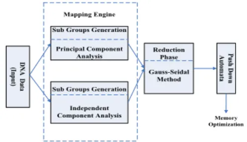
The following figure depicts whole scenario of the current article (Figure 1). Large amount of DNA datasets are chosen here to get optimized output after using different methods. Two methods Principal Component Analysis and Independent Component Analysis are applied distinctly on these datasets. In each methods some parts will partitioned into sub groups generation and reduced. This is occurring by the mapping engine. After completion of processing the previous steps, the Gauss-Seidel method is applied on the dataset and Push down Automata. Ultimately, the methods output as memory optimized and desired result.

Figure 1: Complete Architecture of the propose work

3.1. Principal Component Analysis for DNA

PCA performs a covariance analysis between the factors to reduce the dataset dimensionality. It is an exploratory tool to reduce efficiently multidimensional data sets. It is employed to analyze large multidimensional datasets on gene expression [28-32] as well as to identify mapping and gene sequencing of DNA. It constructs linear combinations of the gene expressions [33]. In the PCA, the number of extracted data is equal to the number of analyzed observed data. For example, for measuring 10,000 genes for 10 persons, this will be formed the largest values of matrix of the10×10,000 measurements. This will be an n×n matrix that can be expressed as follows:

Where p defines the sequence of genes against every person, where the following figure obtained by plotting these 10,000 genes with respect to 10 persons for each of one in multidimensional as illustrated in Figure 2.

Figure 2: The PCs in two dimensional space. In Figure 2, the midline is the principal component that represents the first component. On the other hand, the other line is orthogonal to the first component, so it is the second component. In this way, the other component can be added. In the case of multidimensional data set with large amount of repeated factors, it can be calculated the eigenvectors that is principal components and Eigenvalues as follows:

Where a11, a1n, ann are the eigenvectors with the corresponding eigenvalues λ1, λ2, λn. According to PCA, the gene expression has Gaussian signals, while many gene expression data have ‘super-Gaussian’ signals.

Singular value decomposition (SVD) is a mathematical technique that is closely related to the PCA. It can be applied alternatively on gene expression data. Assume a matrix A of p rows and q columns, thus the SVD for the gene expression data [30-31] as the follows:

Where M is a m*n matrix and VT _{is a n*n matrix.}

The VT contains right singular vector elements and

M contain left singular vector elements. P are

nonzero values on the diagonal and called singular values. Thus, they form ortho-normal basis for gene transcriptional responses.

Since the non-standard application of PCA is accommodating interactions, thus the PCA has been used to investigate in genome analysis. In addition, a standard application, sparse PCA and supervised PCA are in recent approach. In sparse PCA, assume as the first PC, which is given by:

D N A D ata (In pu t)

Sub Groups Generation Principal Component

Analysis

Sub Groups Generation Independent Component Analysis Reduction Phase Gauss-Seidal Method Pu sh D ow n A uto m ata Mapping Engine Memory Optimization ) 1 ..( ... ... 1 1 11 ú û ù ê ë é nn n n p p p p ) 2 .( ... .. 0 0 .. .. .. 1 1 1 11 ú û ù ê ë é ú û ù ê ë é n nn n n a a a a l l ) 3 ...( ... ... T MPV A

-where are non-zero. As the principal components are linear combinations of all genes, all genes have non-zero covariates, where sparse schemes have non-zero coefficients of a few genes.

3.2 .Independent component analysis for DNA The DNA microarrays permit the promising ICA method to measure the transcript activities for a huge number of genes [32-33]. Hughes [34] examined the natural variation in unaltered wild type yeast applied to an extensive dataset that performs 63 ‘neutral’ versus ‘neutral’ experiments. In this experiment, 1464 genes dropped and finalized with 63 4870 data matrix. MacKay [35-36] proposed an ensemble learning ICA approach for easier decomposition can be easily shown:

Where i refers to the original variables given as input, m is the enumerating samples, K allows the Gaussian noise and is the latent variable. For any particular E and F, K provides the reconstruction error, which is given by:

According to the reconstruction error, the data power of latent variables is given by:

Generally, the DNA sequencing represents a cell of all genes as a mixture of independent biological process. Every process forms a vector that shows up-regulation or down-regulation of the gene. Mathematically, it represents linear combination of

n biological processes, where = + +

… + . In matrix form, it can be expressed as follows:

(8) Where

(9)

It can be measured the all gene expression levels in a microarray expression a = (a1,..., a n ) T _{, when a} cell is governed by n independent biological processes s = (s1, ..., s n ) T _{, where each of vector of k} gene levels.

3.3. Push Down Automata

Pushdown Automaton (PDA) is such kind of beneficial tool in computer science that used to free the memory space as it can remember an infinite amount of information. It is basically a finite automaton with a single stack. It is also called push down stack or push down list as it can retrieve stored data. It can read/write a symbol from/in the stack, respectively. PDA has three components, namely input tape, the control unit and infinite size of the stacks. There exists stack head that scans the top element of the stack. Since it is one kind of stack automaton, it has Push-Pop operations. New symbol can be added at the top of the stack with the help of a push function. The pop function reads the top symbol and easily removes that one from the stack. It is done by completing the matching process. There exists stack head that scans the top element of the stack. Typically, PDA maintains the LIFO that is “Last-In First-Out” order. It starts from the uppermost symbol and go ahead with reading one by one from the input tape. The control unit is the major part of PDA that processes the main thing. Once PDA approaches for the next, it reads the symbols and determines whether it is parallel to the stack. If anything is found matches with the symbol of stack pop function meets there and it just doffed out from the stack and rest of the symbols are coming up. In case of not matching the symbol with the stack, it means it cannot belong to the string of input tape. So, if the matches are not found, then that symbol is rejected by the control unit. It is continuing up to the last symbol of the stack. By doing this when it comes to the end, it can be either accepted or rejected. If stack is empty at the ending of input then it accepted by PDA that is it belongs to the string otherwise it is rejected. Consequently, in the present work, three different and substantial methods, namely PCA, ICA and PDA are represented in the same frame by showing time comparisons between them.

Whenever PCA, ICA and PDA are used in large number of dataset for consensus selection, Memory Mapping is another feature to get the goal. It saves the memory depending on match or mismatch that occurs.

3.2. Memory Mapping for Anchor Selection

There are two stacks as input tape and stack. The complete dataset of DNA is kept on the stack table. To save the memory efficiently there exist three units called as count unit, control unit and matching unit. Here, the control unit has the foremost task. It helps to maintain the matching process of the matching unit for the entire dataset of the input tape with the stack. There remains an end indicator or symbol at the end of input table that refers the final ) 4 ...( ... .... 2 2 1 1 1 G G kGk V =h +h + h ) 5 ...( ... ... mi ti mt mi E F K D = + ) 6 ...( ... EF D K= -) 7 ...( ) ( , , , 2 2 2 2 2

å

å

å

å

å

points of the input data set. It determines whether the match is occurring or not and then the control unit doffed out the symbols that either matches or mismatches. In this way, it saves the memory by generating free memory space. It is efficient for finding out the desired seeds using this algorithm. It can manipulate more than hundred base pairs at a time of gene sequence. MMSs stands for Maximum Matching Subsequences. Total DNA datasets are subdivided into small segments to find out the desired parts of the DNA sequences

.

After using above the following methods, Gauss-Seidel Method can be an effective algorithm to find the accuracy in existing dataset. It can provide the proper approximation.

3.3. Gauss-Seidel Method

Gauss-Seidel method is a method that solved linear system with n number of equations with unknown variables. It is also applied in the matrix with nonzero elements. This method is also known as a successive approximation method. This is an optimization method that repeatedly optimized large datasets until reaching a certain points. Assuming zero as the initial approximation set, it is applied in right side of first equation and this result with the rest of the initial approximation is applied in the right side of second equation. When all of the equations process the result, first iteration meets. In order to obtain the desired level of accuracy, it becomes continuous and generates iterations. The

following algorithm demonstrates the Gauss-Seidel method steps.After Gauss-Seidel Method, the Apriori algorithm is used in the current work to determine the frequent item set over the transaction database. It proceeds to identify a frequent item individually with mining the dataset.

3.4. Apriori Algorithm

Assume is the frequent item set and is the candidate item set for size . For each frequent item set, the minimum count is generated with the help of association rule as illustrated in the following algorithm.

Consider a dataset D with data samples (S1,…., S4) converting these segmented data samples into binary flags after comparing with the individual consensus in nucleotide, where each of the consensus is different from another and length of the consensus (A, C, G, T) is also different. Assume that 3.2 minimum supports is obtained, which is 80% and the minimum confidence is 80%. Firstly, the algorithm is used to reach the frequent item set using the Apriori algorithm. Afterward, by manipulating minimum support and confidence, the association rules will be generated. Then finally, the Gauss-Seidel algorithm is applied to obtain the desired iterations. Apriori algorithm is a rule base algorithm that generates targeted items from large set of similar datasets.

Algorithm:1

Memory Mapping (p,q, r, maximum length) Initialize the input symbol (anchor) in input tape (p)

p ← anchor

Initialize MMSs in stack tape (q) q← MMSs

Initialize count unit (r) a ← 0

i← 1 and j ← maximum length while(q[j] == b ) if(p [i] == q[j] ) i← i+ 1and j ← j - 1 if( p[i] == m ) a ← a + 1 p[i] ← p[1] end if else go to line 6. if( q[j] == b ) print r. end if else go to line 6. end if else If ( q[j] == b ) print r. end if else go to line 6 end loop

1

-¬ j

j

An initial guess as output Repeat until convergence For Do ← 0 For j if then ← + End if ← End Algorithm:3

Scan the transaction database to get support, of candidate and compare that with min_ Support to get frequent item set . If is NULL then

Generate all nonempty subsets of 1. Else

Join support to generate candidate and minimum support. For every nonempty subset of 1

4. Implementations and Results

The Core i5 processing speed system has been imposed for parallel computing of two computers. Memories of both computers were of four gigabytes. Java programming language along with Net Beans IDE was used to prepare simulative tools. For each and every datasets length, twenty times simulative executions were performed and finally the average outcomes were recorded in a table. The MySQL database quarries ensure quick datasets alignments from big DNA sequences. A common consensus is determined by applying push down automata. In the present work, ATGCA was used, which is the common for all datasets according to the PDA analysis. Initially, the PCA is compared with rule base approach, the Apriori algorithm. Primary illustrations of Apriori algorithm generate the pre-common sequences.

4.1 Comparisons between PCA and Apriori

Algorithm

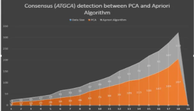
Table 1 reports the numbers of consensus (ATGCA) for different data size using PCA and Apriori algorithm.

Table1: Numbers of consensus (ATGCA) detection by between PCA and Apriori Algorithm

Table 1 portrays that for PCA, the number of values is increased with the increase of the data size. For two billions DNA base pair, the PCA and Apriori provide 17 and 12 counts codes, respectively. For one billion data, there is about

29.41% increase of the PCA identification. . For

three billion DNA base pair, outcomes for PCA and Apriori are 19 and 15, respectively. In this regards, there is about 21.05% increase of PCA, where about

8.36% changes from the previous dataset findings.

For four billion DNA base pair, the findings of the PCA and Apriori are 23 and 17, respectively. Thus, there is about 26.09% increase of PCA with about

5.04% improvements. Consecutively, there are 32.14%, 8.82%, 15.38%, 23.91%, 41.27%, 46.58%, 48.80%, 40.00%, 44.04%, 35.65%, 31.54%, 36.73%, 36.69%and 44.44% increase for

five, six, seven, eight, nine, ten, eleven, twelve, thirteen, fourteen, fifteen, sixteen, seventeen and eighteen billions DNA base pair, respectively of PCA, and 23.32%, 6.56%, 8.53%, 17.36%, 5.31%,

2.22%, 8.80%, 4.04%, 8.39%, 4.11%, 5.19%, 0.04%and 7.75% changes. As the data size

increases, the changes appear, while for the first four data sizes it is decreased, for the 5th _{time it} increased. So, it goes to both upward and downward. From five billion to six billions DNA base pair, the changes are larger than the other part of the DNA base pair. Furthermore, the lowest change is 0.04% that is almost 0 between the sixteen and seventeen billions DNA base pair. The relationships and changes are demonstrated in Figure 3.This 2D graph illustrates the outcomes between used approaches in the table 1.

Figure 3: Coding areas count by PCA and Apriori algorithm.

Figure 3 represents the graphical interface of the selected data size for PCA and Apriori on the other hand, the gray area is the findings from Apriori and the area stair is from the PCA. The orange part is higher than the gray. The maximum values of the PCA is 207. For the Apriori algorithm, the highest value is 325. Figure 3 portrays that from the first step to last step, the PCA findings are greater than that of Apriori. At the first, there are small changes between these two methods However, as time the data size increases, there are significant changes between the PCA and Apriori.

The outputs are nearer to each other in Apriori and it shows few differences for itself. In PCA, the upwards are more than in the Apriori for the 9th _data. There exist high differences of outcomes in it and also in between the two mentioned methods. For the 16th _{data, it crossed over Apriori and continues up to} 18th _{data. Therefore, it is easy to conclude that for} large DNA base pair, the PCA has better capabilities than Apriori for DNA segments findings.

Data Size PCA Apriori

Algorithm 1000000000bp 13 11 2000000000bp 17 12 3000000000bp 19 15 4000000000bp 23 17 5000000000bp 28 19 6000000000bp 34 31 7000000000bp 39 33 8000000000bp 46 35 9000000000bp 63 37 10000000000bp 73 39 11000000000bp 84 43 12000000000bp 95 57 13000000000bp 109 61 14000000000bp 115 74 15000000000bp 130 89 16000000000bp 147 93 17000000000bp 169 107 18000000000bp 207 115

4.2 Impact of PDA with time comparisons in between PCA and ICA

All samples are measured in nanoseconds of time unit. Tables 2 and 3reported the performance of the PCA and the ICA before/after using the PDA; respectively, in terms of the consumed in data samples.

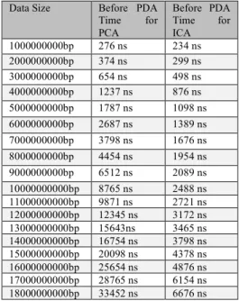
Table 2: Time comparisons between PCA and ICA before applying PDA

Data Size Before PDA

Time for PCA Before PDA Time for ICA 1000000000bp 276 ns 234 ns 2000000000bp 374 ns 299 ns 3000000000bp 654 ns 498 ns 4000000000bp 1237 ns 876 ns 5000000000bp 1787 ns 1098 ns 6000000000bp 2687 ns 1389 ns 7000000000bp 3798 ns 1676 ns 8000000000bp 4454 ns 1954 ns 9000000000bp 6512 ns 2089 ns 10000000000bp 8765 ns 2488 ns 11000000000bp 9871 ns 2721 ns 12000000000bp 12345 ns 3172 ns 13000000000bp 15643ns 3465 ns 14000000000bp 16754 ns 3798 ns 15000000000bp 20098 ns 4378 ns 16000000000bp 25654 ns 4876 ns 17000000000bp 28765 ns 6154 ns 18000000000bp 33452 ns 6676 ns

Table 2 depicts that before applying PDA into the data samples, the data takes 276 ns time using PCA, whereas 234ns using ICA. Consequently, ICA needs less time than PCA to generate the result and for this data; PCA takes 42 ns more than the ICA. In the same way, ICA takes 299 ns which is75 ns less than PCA for the second data size. The third data in Table 3 shows 156 ns as difference. Moreover, the differences of PCA and ICA for the same data sizes are 361, 689, 1298, 2122, 2500, 4423, 6277, 7150,

9173, 12178, 12956, 15720, 20778, 22611 and 26776, respectively. As checking for large datasets,

the differences are increasing in an incessant way that is PCA takes time more than ICA that increases ultimately.

Table 3: Time comparisons between PCA and ICA after applying PDA

Data Size After PDA

Time for PCA After PDA Time for ICA 1000000000bp 198 ns 145 ns 2000000000bp 212 ns 167 ns 3000000000bp 345 ns 243 ns 4000000000bp 643 ns 354 ns 5000000000bp 1009 ns 543 ns 6000000000bp 1564 ns 678 ns 7000000000bp 1975 ns 712 ns 8000000000bp 2675 ns 899 ns 9000000000bp 3078 ns 1045 ns 10000000000bp 3975 ns 1387 ns 11000000000bp 4876 ns 1567 ns 12000000000bp 5576 ns 1897 ns 13000000000bp 6782 ns 2012 ns 14000000000bp 7854 ns 2187 ns 15000000000bp 8812 ns 2234 ns 16000000000bp 9123 ns 2476 ns 17000000000bp 9654 ns 2688 ns 18000000000bp 9912 ns 2978 ns

According to Table 3, first data take 198ns time for PCA, whereas ICA needs to take 145 ns after attaching PDA. Therefore, a time difference of 53 ns is required less for ICA than PCA. Similarly, for the second data size, ICA takes 167 ns which is also 45 ns less than PCA. For the third dataset, the table shows 102 ns as time difference. Additionally, the differences of PCA and ICA for the same data sizes are 289, 466, 886, 1263, 1776, 2033, 2588, 3309,

3679, 4770, 5667, 6578, 6647, 6966 and 6934,

respectively, that actually indicates ICA after combining PDA as more efficient and time consuming.

4.3 Association Rule

Currently, generate the association rules for frequent item sets from L3. For every item sets of L3, all nonempty subsets of frequent item sets are generated. Consider N = {A, C, T}, then it’s all nonempty subsets are:

{A}, {C}, {T}, {A, C,}, {C, T}, {A, T}. Considering minimum confidence threshold is 80%.The resulting association rules are shown below: Rules Confidenc e Status Result R1:A^C→T 4/4=100% Selected R2: A^T→C 4/5=80% Selected R3: C^T→A 4/4=100% Selected R4: A→C^T 4/5=80% Selected R5: C→A^T 4/5=80% Selected R6: T→A^C ………… 4/7=57.14 % ………… …. Rejected ………..

Thus, the flags of D1 dataset are:

SID A C G T

S1 2 1 0 2

S2 1 2 1 1

S4 1 1 0 3 It can be written using the following equations:

(10)

These equations can be rewritten as:

₍₁₁₎

In this system applying Gauss-Seidal method obtain the successive iterations as follows:

First iteration: (2.50000, 1.25000, 0.62500, 0.43250) Second iteration: (1.44250, 1.25000, 0.93750, 0.78147) Third iteration: (1.09353, 1.09375, 1.01563, 0.94820) Fourth iteration: (1.00493, 1.01563, 1.01563, 1.00322) Fifth iteration: (0.98897, 0.99609, 1.00586, 1.01493) Sixth iteration: (0.98702, 0.99609, 1.00098, 1.01557)

For the third dataset D2 with segmented data samples will be generated.

SID Consensus

S1 AACCTA

S2 CAGCGT

S3 CTACAG

S4 CGTTAC

If elements of sequence are presented in sample then put 1, otherwise 0. By doing convert the attributes into binary flags:

SID A C G T

S1 3 2 0 1

S2 1 2 2 1

S3 2 2 1 1

S4 1 2 1 2

Scan the dataset D2 to count each candidate and then comparison. Thus, C1 and L1 are generated:

From L1, the two frequent patterns of sequence, C2are generated, then scan the dataset D2 to obtain support countL2.

After getting C2 and L2, generatesmin_supportL3, then classify the different gene class.

L3 indicates one classify group that satisfy our considerable support_count. Apply the association rule considering the desirable confidence value. From the preceding results, it is established that the Gauss-Seidal method is iteratively simulates the DNA datasets so that common segment can be easily determined. Consensus is the segment that has most common DNA pattern. Simulative operation among training DNA data by Gauss-Seidal ensure desired consensus. Association rules permit automated environment for handling new testing and training

L2

Nucleot

ide _Count Support

{A} 7 {C} 8 {G} 4 {G} 4 {T} 5 {T} 5 Comparing Support_Count with min_support

data. New rules are generated for upcoming datasets and problems. PCA and ICA help to map the whole DNA segments. According to the analysis, ICA performs better than PCA.

4. Conclusion

The current work proposed an approach for selecting a consensus from big dataset. This approach provides the opportunities to manipulate vast amounts of data with mapping facilities as an outcome. Large data formulation within a short time is the key feature of the present work. Saving memory space by having access to the manipulation facilities of large data is another laudatory feature.

Different algorithms and methods were applied to achieve successful results. Pushdown Automata makes the whole process more efficient and time saving. It provides the exact mapping facilities remaining other facilities same as before. Applying Gauss-Seidel method seems like epoch implementation, where it is entirely great innovation that helps in saving the memory as well as time. It makes the idea more impactful and genuine. Using this method that combines the other together lastly makes this work more strong and powerful. It helps to contribute greatly since it establishes the desired path way as a result. According to the experimental dataset with the result, it fulfills the proposal firmly. Maximum 18000000000bp was taken here as experimental data size in DNA sequencing. Though big data inserted in the current work are used to examine and to analyze the ultimate procedure, it is not possible to get the same result with facilities when it is crossed the maximum data size over. The faster way that achieved can be slow to complete execution. In that case, it fails to get the exact features. In future, we will consider the Brain datasets along with DNA data to find out the disease centric biological problem. In future, we will consider the Brain datasets along with DNA data to find out the disease centric biological problem.

References

[1]. A.Turcu, R. Palmieri,B. Ravindran, S. Hirve, Automated Data Partitioning for Highly Scalable and Strongly Consistent Transactions, IEEE Transactions on Parallel and Distributed Systems,Vol.27, No.1,pp.106-118, 2016.

[2]. S.P. Deng,L. Zhu , D.S. Huang, Predicting Hub Genes Associated with Cervical Cancer through Gene Co-Expression Networks, IEEE/ACM Transactions on Computational Biology and Bioinformatics, Vol.13, No. 1,pp.27-35, 2016

[3]. S.Y.Hsieh,Y.C. Chou, A Faster cDNA Microarray Gene Expression Data Classifier for Diagnosing Diseases, IEEE/ACM Transactions on Computational

Biology and Bioinformatics, Vol.13, No. 1,pp.43-54, 2016

[4]. N. Dhulekar, S. Ray, D. Yuan, A. Baskaran, B. Oztan, M. Larsen, B. Yene, Prediction of Growth Factor-Dependent Cleft Formation During Branching Morphogenesis Using A Dynamic Graph-Based

Growth Model, IEE/ACM Transactions On

Computational Biology And Bioinformatics, vol. 13, no. 2,pp.350-363,2016.

[5]. J. A. Saez, M. Galar, J. Luengo, F. Herrera, INFFC: An iterative class noise filter based on the fusion of classifiers with noise sensitivity control, Information Fusion, vol. 27, 505-636, 2016.

[6]. J.A. Sáez, J. Luengo, F. Herrera. Evaluating the classifier behavior with noisy data considering performance and robustness: The Equalized Loss of Accuracy measure, Neurocomputing, vol 176, pp. 26-35, 2016.

[7]. Palacios, L. Sanchez, I. Couso. An extension of the FURIA classification algorithm to low quality data through fuzzy rankings and its application to the early diagnosis of dyslexia. Neurocomputing, vol. 176, 2016, pp.60-71, 2016.

[8]. D. Martin, J. A. Fdez, A. Rosete, F. Herrera, NICGAR: a Niching Genetic Algorithm to Mine a Diverse Set of Interesting Quantitative Association Rules, Information Sciences, vol. 355-356, pp.208-228, 2016.

[9]. M. González, C. Bergmeir, I. Triguero, Y. Rodríguez, J.M. Benítez, On the Stopping Criteria for k-Nearest Neighbor in Positive Unlabeled Time Series Classification Problems, Information Sciences, vol. 328,pp.42-59, 2016.

[10]. http://www.chemguide.co.uk/organicprops/aminoacids /doublehelix.gif

[11]. B. Akbal-Delibas1, R. Farhoodi1, M. Pomplun1, N. Haspel1, Accurate refinement of docked protein complexes using evolutionary information and deep learning, Journal of Bioinformatics and Computational Biology, Volume 14, Issue 03, pp.1-14, June 2016. [12]. B. Wang, M. Wang, Y. Jiang, D. Sun, X. Xu, A novel

network-based computational method to predict protein phosphorylation on tyrosine sites, Binghua Wang et al, J. Bioinform. Comput. Biol. volume 13, 1542005, 2015.

[13]. D. Wang, J. Hou, Explore the hidden treasure in protein–protein interaction networks — An iterative model for predicting protein functions, Journal of Bioinformatics and Computational Biology, Volume 13, Issue 05, October 2015.

[14]. J.D.I. Watson, R.A. Laskowski, J.M.Thornton, Predicting protein function from sequence and structural data, CurrOpinStruct Biol. 2005 Jun;15(3):275-84.

[15]. N. Kalra and A. Kumar, State Grammar and Deep

Pushdown Automata for Biological Sequences of Nucleic Acids, Current Bioinformatics, 2016, 470-479.

[16]. M. Hague, A. S. Murawski, C.H. L. Ong, and O. Serre, Collapsible Pushdown Automata and

Recursion Schemes, ACM Trans. Comput. Logic

2017, 42 pages.

[17]. R. Hubley, R. D. Finn, “The Dfam database of repetitive DNA families”, Nucleic Acid Researchs, vol 2015, 81-89.

[18]. P. Bailis, C. Fournier, J. Arulraj, A. Pavlo, “Distributed Consensus and Implications of NVM on Database Management Systems”, Communications of the acm, 2016.

[19]. J. Dutkowski, A. Gambin, “On consensus biomarker selection: on consensus biomarker problem”, BMC Bioinformatics, 8 suppl 5:S5, 2007.

[20]. S. Kim, M. Con, H. Kang, “A method for generating new datasets based on copy number for cancer analysis”, BioMed Research Int., 2015 .

[21]. J. Bendl, J. Stourac, “Predict SNP: Robust and Accurate Consensus Classifier for Prediction of Disease-Related Mutations”, PLOS Computational Biology,2014.

[22]. H. Sobhy, “Shetti, a simple tool to parse, manipulate and search large datasets of sequences”, Microbial Genomics, 2015.

[23]. Z. Yu ,H. S. Wong, H. Wang, “Graph-based consensus clustering for class discovery from gene expression data”, Bioinformatics, 2007, 2888-2896.

[24]. A. Arnedillo, Ruben Calvo Molinos, Borja Inza Cano, Iñaki LópezHoyos, Marcos Martinez Taboada, Víctor Ucar, Eduardo Bernales, Irantzu Fullaondo, Asier Larrañaga Múgica, Pedro Zubiaga, Ana María - “Microarray analysis of autoimmune diseases by machine learning procedures”, Ieee Transactions on Information Technology in Biomedicine, ISSN 1089-7771, 2009.

[25]. A. Figueras, D. Robledo, A. Corvelo, “Whole Genome Sequencing of Turbot (Scophthalmusmaximus; Pleuronectiformes): A Fish Adapted to Demersal Life”, DNA Research, Oxford Journals, 2016. [26]. L. tolosi, J. Theiben, “A method for finding consensus

breakpoints in the cancer genome from copy number data”, Bioinformatics, 2013, 1793-1800.

[27]. G. Hovel-Miner, M. R. Mugnier,...,“A Conserved DNA Repeat Promotes Selection of a Diverse Repertoire of Trypanosomabrucei Surface Antigens from the Genomic Archive”, PLOS Genetics, 2016. [28]. B. R. Anderson, P. Chopra, “Identification of

consensus binding sites clarifies FMRP binding determinants”, Nucleic Acid Research, 2016, 6649– 6659.

[29]. J. IT. “Principal Component Analysis.” New York: Springer, 1986.

[30]. R.A. Johnson, D.W. Wichern, Applied Multivariate Statistical Analysis, Upper Saddle River, NJ: Prentice Hall, 2001.

[31]. K.Pearson, On lines and planes of closest fit to systems of points in space, PhilosophicalMagazine, 1901, 559-572.

[32]. C.Bishop, Pattern Recognition and Machine Learning.” Springer-Verlag, 2006.

[33]. S.Haykin, S. “Modern Filters.” Macmillan, 1989. [34]. B. Grung, R. Manne, “Missing values in principal

components analysis.” Chemo- metrics and Intelligent Laboratory Systems, 1998, 125-139.

[35]. I.T. Jolliffe, B. Jones, and B.J.T. Morgan, Cluster analysis of the elderly at home: a case study.” Data Anal. Inform., pp. 745-757, 1980.

[36]. S.Knudsen, “Cancer Diagnostics with DNA Microarrays.Hoboken,” NJ: John Wiley and Sons, 2006.

[37]. G.J. McLachlan, D. KA, Ambroise C. “Analyzing Microarray Gene Expression Data.” Wiley Interscience, 2004.