Rheological characterization of polymer-graphene nanocomposites

(1)

Dušan Fetih

Rheological Characterization of

Polymer-Graphene Nanocomposites

Dušan Fetih

4

(2)

(3)

(4)

(5)

Abstract

Graphene is one of many nanofillers often incorporated in polymeric matrixes in order to produce polymer nanocomposites. In the time being, melt compunding (e.g., via extrusion) is accepted as the most promising method to produce such materials at a large-scale production scenario. However, since correlations between processing conditions and nanocomposite morphology remains unclear, a general procedure for controlling the final characteristics of these materials to a specific application is still lacking. The main goal of this thesis is to understand how dispersion of polymer/graphene nanocomposites is affected by the processing conditions used on a twin screw extruder. Samples were collected along the axial length of the extruder in order to monitor the evolution of dispersion by means of Small-Amplitude oscillatory shear (SAOS) measurements and bright-field microscopy performed at the lab. Effects of graphene type, feed rate, screw speed, and the evolution of dispersion along the extruder were analyzed. Additionally, the off-line rheological measurements were compared with on-line measurements that were undertaken within the scope of a bigger project done in cooperation with BASF. It is concluded that both graphene types induce a shear thinning behavior over the entire range of frequencies considered and enhanced dispersion is achieved with smaller particle size graphene. Moreover, lower feed rates and lower screw speeds induce better dispersion levels. Furthermore, dispersion is partially improved along the extruder and discrepancies between on-line and off-line results were found.

(6)

(7)

Resumo

O grafeno é um dos vários reforços à escala nanométrica que é incorporado em matrizes poliméricas de forma a produzir nanocompósitos. Atualmente, os processos de composição no fundido (p.e., através de extrusão) são aceites como os métodos mais promissores na preparação destes materiais, no cenário de produção em larga escala. Contudo, uma vez que não são claras as correlações entre as condições de processamento e a morfologia dos nanocompositos, falta ainda estabelecer procedimentos para controlar as características finais destes materiais numa aplicação específica. O objetivo principal desta tese é compreender como a dispersão em nanocompósitos de polímero com grafeno são afetadas pelas condições de processamento usadas numa extrusora de duplo-fuso. Foram recolhidas amostras ao longo do comprimento axial da extrusora, de forma a monitorizar a evolução da dispersão através de medições feitas no laboratório de reologia oscilatória (SAOS) e microscopia de campo claro. Foram analizados o efeito do tipo de grafeno na composição, o débito, velocidade dos fusos, e a evolução da dispersão ao longo da extrusora. Para além disso, as medições off-line foram comparadas com medições on-line realizadas no âmbito de um projeto colaborativo com a BASF. Foi concluído que ambos os tipos de grafeno induzem o comportamento pseudo-plástico ao longo de toda a gama de frequencias usadas e houve uma melhoria da dispersão com o grafeno possuindo um tamanho de partícula inferior. Além disso, a dispersão é parcialmente melhorada ao longo da extrusora and foram encontradas discrepâncias entre os resultados on-line e off-line.

(8)

(9)

List of figures

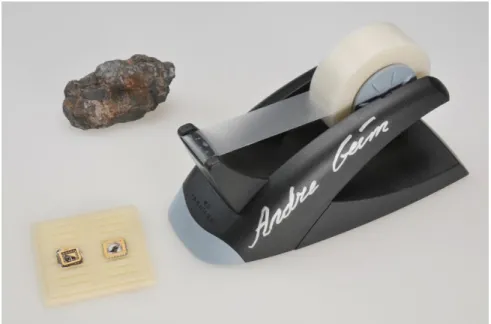
Figure 1: A lump of graphite, a graphene transistor and a tape dispenser ... 14

Figure 2: Visual representationof graphene ... 15

Figure 3: Graphene as the building block of all graphitic forms ... 16

Figure 4: Dynamic Frequency Sweep of PEN ... 22

Figure 4.1: Complex viscosity curves of the neat nylon 6 ... 27

Figure 4.2: Effect of reprocessing on G’,G’’ and η* of the PC/MWCNT... 29

Figure 5: Leistritz LSM 30.34 extruder ... 32

Figure 6: Screw profile with extruder barrel setup ... 33

Figure 7: Disk mold with the final sample ... 35

Figure 8: Materials used and final shape after molding ... 35

Figure 9: Leitz® 1401 microtome ... 36

Figure 10: Cured microscopy samples... 36

Figure 11: AR-G2 rheometer ... 37

Figure 12: Linear viscoelastic regimes of Formulation 5 ... 38

Figure 13: Microscope, software and camera used ... 39

Figure 14: First stage in data processing of Formulation 4... 39

Figure 15: Second stage in data processing of Formulation 4 ... 40

Figure 16: Third stage in data processing of Formulation 4 - tanδ ... 41

Figure 17: Final look of after the data processing ……….41

Figure 18: Comparison of G’ and G’’ for formulation 1, 2 and 6 ……….42

Figure 19: Comparison of η, for formulation 1, 2 and 6……….43

Figure 20: Comparison of G’ for a)Form.5 and 9 and b)Form.4 and 8 …..………44

Figure 21: Comparison of η* for c)form. 5 and 9 and d) form. 4 and 8 …………..……44

Figure 22: Comparison of formulation 2 and 4 for a)G’ and b) G’’ ……….45

Figure 23: Comparison of complex viscosities for formulation 2 and 4 ……….46

Figure 24: Comparison of formulation 6 and 8 for a)G’ and b) G’’ ……….……….46

Figure 25: Comparison of complex viscosities for formulations 6 and 8 ……….47

Figure 26: Comparison of formulations 2 and 3 for a)G’ and b) G’’ ……….48

Figure 28: Comparison of formulations 6 and 7 for a)G’ and b) G’’ ……….49

Figure 30: Storage modulus for all formulations at L/D 15,17,24 ………..52

Figure 31: Micrograph of form. 5, L/D=15, 17 and 24, from the barrel ……….53

Figure 32: Micrograph of form. 5, L/D=15, 17 and 24, after comp.molding ….……….54

Figure 33: G’,G’’ and η* for a)off-line and b)on-line PA ……….54

Figure 34: G’,G’’ and η* for a) off-line and b)on-line formulation 2 ……….55

(14)

(15)

List of tables

Table 1: Most relevant properties od Ultramid® A3W ... 41

Table 2: Formulations used in this work in terms of weight percentages ... 42

Table 3: All formulations in terms of graphene type ... 42

(16)

(17)

Acknowledgements

First and foremost I would like to convey my sincere gratitude to my mentor, professor José A. Covas (Department of Polymer Engineering, University of Minho) and to my adviser Sacha T. Mould, PhD (Department of Polymer Engineering, University of Minho) for their irreplaceable scientific guidance and generous personal support, great patience and understanding.

I would also like to thank professor Igor Emri (CEM, University of Ljubljana) for his passionate lectures that encouraged me to explore the vast fields of rheology in my first year of EURHEO studies. My thanks also goes to professor Paula Moldenaers (KUL, University of Leuven) for her methodic and clear lectures on Experimental Techniques in the second year of EURHEO.

I would like to use this opportunity to once more express my thankfulness for the unique chance that was given to me by the EURHEO consortium and for awarding me with an Erasmus Mundus scholarship. I can say with confidence that my EURHEO experience was life changing in every sense of the word.

Special thanks to the secretary, Ms. Patrícia Cavaco that made all the daunting communication, paperwork and documentation tasks so easy for us, the students.

My sincere thanks to the research group at the Department of Polymer Engineering at the University of Minho for their friendliness and willingness to help. Special thanks go to the department technician Mr. João Paulo.

(18)

(19)

Preface

This thesis stands as a crown achievement of a two year Erasmus Mundus Master Course in Engineering Rheology - EURHEO. It also marked an end of a wonderful two year journey filled with many unforgettable adventures, lifelong friendships and passion for studying and excellence. The thesis was completed in its entireness at the Department of Polymer Engineering at the University of Minho, Portugal, a proud member of the EURHEO consortium.

EURHEO program combines the expertise of six leading European Universities in the field of Rheology – Universidade do Minho (Portugal), Katholieke Universiteit Leuven (Belgium), Univesidad de Huelva (Spain), Univesita Degli Studi Della Calabria (Italy),

Univesite Catholique de Louvain (Belgium) and Univerza v Ljubljani (Slovenia).

My personal higher institution path inside the Eurheo Erasmus Master Program included University of Ljubljana for the first year and University of Minho for the second year of the program.

The aim of Eurheo program is to provide a cutting edge education in multidisciplinary fields of rheology and its application to a variety of engineering disciplines.

(20)

(21)

Dedicatory

To my mother, Nadežda, a great fighter, a truly remarkable woman and to my father Dušan (R.I.P) I send my deepest thoughts for all the support, encouragement and love throughout my life and my studies.

To the one who stole my hart, Jovana.

My thanks also go to all of my colleagues and friends from the 5th_{EURHEO generation:}

Evgeniy Liashenko, Tesfalidet Gebrehiwot, Michaela Turcanu, Taisir Shahid, Farah Haseeb, Domenico Lupo, Gabriel Ferrante, Sergio Carillo de Hart, Joris Betjes, George and Emanuel and to all the wonderful people that I met during this two unforgettable years. Among others: Joamin Gonzales, Prakhyat Heymady, Weronika Wojtak, Jure Kobal, Marko Bek, Alen Oseli, Marina and Ivan Saprunov and Alexandra Aulova.

(22)

(23)

Chapter 1: Introduction

1.1 Motivation

By nanocomposite one mainly refers to a multiphase material where one of the phases has at least one of its dimensions at the nanometer scale [1]. As a result of the extraordinary high surface to volume ratio of the dispersed phase, nanocomposite materials differ substantially from conventional composites. In comparison to the typical composite materials the area of the interface between the dispersed and the matrix phase is generally an order of magnitude greater. There are many documented advantages of nanocomposites so just a few properties that undertook the most major improvements will be stated: mechanical properties (e.g. strength, modulus), better thermal stabilization, decreased permeability, increased electrical conductivity, flame retardancy and many more [2].

Because of the numerous improvements that nanocomposites brought, there has been an ever increasing interest for these materials from the side of automotive and many other industries and the pressure was put on scientists and researchers worldwide to develop novel materials as well as to investigate and understand more deeply the existing ones. In the large field of nanotechnology, polymer matrix based nano composites have become an important area of current research and development [3]. Various fillers are commonly used to modify polymer properties and upgrade the performance of polymeric systems. Graphene is one of many nano filler materials often incorporated in polymeric matrix in order to produce graphene/polymer nanocomposites. In order to properly utilize these highly promising materials in the times to come, the critical focus will be on the ability to compound and process them into desired forms and shapes with adequate properties. From an economic stand point, the ability to use conventional melt processing techniques such as extrusion and injection molding will play a significant role since the science and technologies behind the composite polymer processing are well established and understood. Despite the major influence of

(24)

processing parameters on the final nano composite properties, a relatively few reports have considered their effects. In writing of the thesis it proved challenging to objectively compare and generalize conclusions deriving from scarce and completely different sources.[2] Thorough search of the currently available literature showed that relatively little can be found on the relationships of the degree of mixing, processing parameters and final graphene/polymer nano composite properties.

To summarize, the main focus of this thesis is to investigate and understand the intricate details behind the general dispersion levels achieved by twin screw extrusion. As side objectives, evolution of dispersion and the effects of operating conditions were studied. Investigative means used to accomplish the task consisted of small amplitude oscillatory shear (SAOS) measurements were used for off-line rheological characterization accompanied by bright field microscopy. In a framework of a broader project, a series of on-line and electrical resistivity measurements were performed. Some of the results were used in subsequent chapters for comparative analysis between the obtained on-line and off-on-line results.

(25)

1.2 Objectives of the work

The objective of this thesis is focused at the rheological properties of graphene/polymer nanocomposites as a mean to better understand dispersion levels achieved by twin screw extrusion. The main objectives of the thesis are summed below:

 Study viscoelastic properties of graphene/polymer nanocomposites and correlate the rheological responses to dispersion levels.

 Study evolution of the rheological properties along the twin screw extruder.

 Understand how the processing conditions affect dispersion levels and their evolution along the twin screw extruder.

(26)

1.3 Outline of the thesis

This thesis consists of 5 chapters and appendix. Chapter 1 is dedicated to brief introduction of the reader to the aim and objectives of the work. It provides information about nanocomposites in general, their advantages, disadvantages, applications, relevance and future industrial prospects. Chapter 2 presents an overview of the current state of the art on co-rotating intermeshing twin screw extruders and their mixing and dispersion capabilities, graphene and graphene/polymer nano composites and previous work done on the preparation of graphene nanocomposites by twin screw extrusion. Chapter 3 covers experimental part of the work. It presents the materials used, procedures utilized to prepare the nanocomposites and the characterization techniques. Chapter 4 analyses the obtained results and discusses the influence of different processing conditions and formulations. It compares relevant off-line and on-line measurements and microscopy data. Chapter 5 is reserved for concluding remarks and proposed future work. Finally, we have references cited and the appendixes that show all the data that were obtained during measurements but did not find their way in the main chapters due to their lower importance.

(27)

Chapter 2: Literature survey

2.1 General overview

The field of Nano science has prospered over the last few decades. The applications of nanotechnology managed to found their ways in areas such as computing, sensors, and biomedical applications [3]. In this highly competitive world, academic and industrial researchers can be found in constant pursuit to provide added properties to the neat polymers, without sacrificing its processability or adding excessive weight [4].

Conventional composites require, in general, a large amount of additives in order to influence important changes in the properties of the polymeric systems. On the other hand, nanocomposites are formed by the dispersion of a relatively small amount of nanofiller into the polymer matrix (1 to 5% of the mass fraction) [5]. This completely new generation of fillers exhibits at least one characteristic length at the order of nanometer and they come in a variety of shapes raging from isotropic to highly anisotropic. Based on the shape criterion, nanofillers are categorized as nanospheres, nanotubes, nanowires, nanofiber and nano-platelets [6].

In constantly changing field of nanocomposites, carbon black, carbon nanotubes and layered silicates are the fillers that have been used most extensively to improve mechanical, thermal, electrical and gas barrier properties of polymer matrices [7,8,9]. The discovery of graphene had a big impact on nanocomposite world. With the combination of extraordinary physical properties and ability to be dispersed in various polymer matrices it has created a new type of polymer nanocomposites – polymer/graphene nanocomposites [10,11]. Scientific community has been theorizing about graphene for several decades [12]. From H.P. Boehm who coined the term Graphene in 1962 to a remarkable breakthrough in isolation of graphene by Andre Geim and Konstantin Novoselov in 2003 [12,17]. This marked a beginning of a new era in scientific research of extraordinary properties behind the material. Six years after their groundbreaking isolation of graphene, the two were awarded a Nobel Prize in Physics for their work in revealing this new two-dimensional material (see Fig. 1).

(28)

Figure 1: A lump of graphite, a graphene transistor and a tape dispenser. Donated to the Nob el Museum in Stockholm

(29)

2.2 Graphene

Carbon nanofillers can be separated corresponding to the dimensionality of the material. Carbon molecules such as fullerenes – 0D, carbon nanotubes – 1D, graphene macromolecules – 2D and carbon materials such as diamond and graphite – 3D [13]. Many graphene-based nanoparticles could be appropriate for nano composite production. The list mainly includes nanofillers derived from graphite nanoplatelets, graphite intercalation compounds and graphene oxide [14].

Because of their excellent properties and natural abundance of the precursor graphite, graphene sheets emerged as a reasonable alternative to the carbon nanotubes, for production of functional nanocomposites [15].

Graphene can be defined as a one atom thick layer of graphite with sp2_-hybridized

carbon atoms arranged in a six numbered ring plane (see Fig. 2) [16].

Figur e 2

Figure 2: On the left, unprocessed atomic resolution a) experimental raw BF, b ) simulated BF, c) simulated HAADF

and d) raw experimental HAADF images of pristine single layer graphene at 60kV; On the right, visual representation

of Graphene honeycomb lattice. (Taken from R.Zan, Q.M. Ramasse, R.Jalil and U.Bangert- Atomic Structure of

Graphene and h-BN Layers and Their Interactions with Metals [77])

Some researchers see graphene as the building block of all other graphitic carbon allotropes of different dimensionality [17].

To illustrate, graphite, a 3D carbon allotrope, is essentially made up of graphene sheets stacked on top of each other and separated by just a few angstroms a part (3.37A˚). The 0D carbon allotrope, fullerenes, can be envisioned as if they are made by wrapping a

(30)

section of graphene sheet in order to form a sphere. Carbon nanotubes (CNT) and nanoribbons (1D carbon allotropes), can be obtained by rolling and slicing graphene sheets, respectively (see Fig. 3).

Figur e 3

Figure 3:Graphene, the b uilding b lock of all graphitic forms, can b e wrapped to form the 0-Db uckyb alls, rolled to form

the 1-D nanotub es, and stacked to form the 3-D graphite. Copyright Nature Pub lishing Group – picture taken from H.Kim, A.A. Ab dala,C. W. Macosko - Graphene/Polymer Nanocomposites [44]

However, in reality, all these carbon allotropes, with the exception of nanoribbons, are not synthesized directly from graphene [18].

With the Young’s modulus of 1 TPa and ultimate strength of 130 GPa, single-layer graphene is the strongest material ever measured [19]. It has a thermal conductivity of 5000 W/(m3K), which corresponds to the upper bound of the highest values reported for SWCNT bundles [20]. Moreover, single-layer graphene possesses a very high electrical conductivity, up to 6000 S/cm [21], and in contrast to carbon nanotubes, chirality is not a factor in its electrical conductivity. All this extraordinary properties are accompanied by extremely high surface area (theoretical limit: 2630 m2/g) and gas impermeability [22]. So far, there are two established approaches to synthetize graphene. Namely, bottom-up and top-down approach. In bottom-bottom-up processes, graphene is synthesized by a variety of methods such as chemical vapor deposition (CVD)[23], arc discharge [24],

(31)

epitaxial growth on SiC [25], chemical conversion [26], reduction of carbon oxide [27], unzipping carbon nanotubes [28], and finally, self- assembly of surfactants [29].

From afore mentioned techniques, CVD and epitaxial growth proved to be capable of producing minute amounts of large size, defect free graphene sheets. Although, CVD and epitaxial growth can be used for fundamental studies and applications in high end electronics, they are not suitable for polymer nanocomposites that demand large quantities of graphene sheets.

On the other side, with the top-down approach, graphene or modified graphene sheets are produced by separation/exfoliation of graphite or graphite derivatives [30]. In these procedures, the starting position is graphite or its derivatives which offers significant economic advantage over the bottom-up methods. As a whole, these methods are more suitable for large scale production that is required for polymer composite applications.

2.2.1 Direct exfoliation of Graphite

Micromechanical cleavage of graphite gave birth to the interest in graphene [31]. The procedure is capable of producing large size, high quality sheets but in very limited amounts, which makes it suitable only for fundamental studies or electronic applications. However, recently graphite has also been directly exfoliated to single and multilayer graphene with sonication in the presence of polyvinylpyrrolidone [32] or N-methylpyrrolidone [33], electrochemical functionalization of graphite assisted with ionic liquids [34], and through dissolution in superacids [35].

The direct sonication method has presented a potential to be scaled up to produce large quantities of single and multilayer graphene or functionalized graphene that can be used in nanocomposite applications. However, all these techniques come with downsides that could prove to be quite challenging and difficult to overcome. The dissolution of graphite in chlorosulfonic acid [35] has a great potential for a large scale production but the hazardous nature of the hydrosulfonic acid and the costs of its removal may hinder its potential.

(32)

2.2.2 Graphite Oxide (GO)

Currently, the most promising methods for large scale production of graphene are based on the exfoliation and reduction of graphite oxide. In analogy to graphite, which is composed of stacks of graphene sheets, graphite oxide is composed of graphene oxide sheets stacked on one another [36].

The structure of graphene oxide has been the subject of many theoretical [37,38] and experimental studies [39,40,41]. The reader is referred to Dreyer et.al [42] for more details on graphite oxide and its preparation, structure, and reactivity.

Exfoliation of graphite oxide in order to produce chemically modified graphene sheets offers different ways for large scale production of functionalized graphene sheets. Although graphite oxide can be relatively easily dispersed in water [43] and in organic solvents, graphene oxide is electrically insulating and thermally unstable. Thus, at least partial reduction of graphene oxide is necessary to restore electri cal conductivity. A number of different methods currently exist for the exfoliation and reduction of GO to produce chemically modified graphene. The methods are: chemical reduction and thermal exfoliation and reduction.

Chemical reduction – a stable colloidal dispersion of graphite oxide is produced followed by chemical reduction of the exfoliated graphene oxide sheets. Stable colloids of graphene oxide can be obtained using solvents such as water, alcohol and combined with either sonication or long stirring. While these suspensions can be used for production of GO based polymer composites, the low electrical conductivity and poor thermal stability of graphene oxide are significant drawbacks [44].

Thermal exfoliation and reduction – Thermally reduced graphene oxide (TRG), can be produced by rapid heating of dry graphite oxide under inert gas and high temperature [45,46]. Heating of graphite oxide is performed in an inert environment at 1000°C for about 30 seconds leads to reduction and exfoliation of GO - producing TRG sheets. There is around 30% weight loss that is associated with the decomposition of the oxygen groups and evaporation of water [45].

(33)

The exfoliation leads to volume expansion of up to 300 times, producing very low-bulk- density TRG sheets [45].

The main advantage of the thermal reduction methods is the ability to produce chemically modified graphene sheets without the need for dispersion in a solvent. The thermal reduction also leads to restoration of the electrical conductivity [45].

To summarize, it is indicative that the most promising routes to preparation of graphene for polymer nanocomposites start from graphite oxide although, chemically modified graphene materials can prove challenging for proper melt compounding due to their proneness to thermal degradation. Due to thermal instability of most chemically modified graphene, use of melt blending has so far been limited to a few studies with the thermally stable Thermally Reduced Graphene Oxide.

(34)

2.3 Polymer/graphene nanocomposites

Graphene and its derivatives as fillers for polymer matrix composites have shown a great potential for a range of applications. In the past few years, researches have made successful attempts at producing GO and graphene/polymer nanocomposites similar to carbon nanotube (CNT) based polymer composites.

Since graphene has better electrical, thermal and mechanical properties as well as higher aspect ratio and larger surface area than other reinforced materials such as carbon fibers and Kevlar® Its reinforcement can offer exceptionally better properties for specific applications [47].

The recent advancement in bulk synthesis processes of graphene and RGO has generated great interest to incorporate such unique material into various polymeric matrices.

The majority of graphene based nanocomposites have been developed using the three following methods: solvent processing, in situ polymerization and melt processing [15]. The most economically attractive, scalable and environmentally friendly method for dispersion of nanoparticles into polymers is melt blending.

Dispersion of the original agglomerates of the nanofiller represents braking down to smaller agglomerates or individual particles during mixing by the action of the flow forces. This may prove to be a challenging task since, the Individual nanofiller particles can exhibiting large cohesive forces and require considerable energy or mechanical stress to achieve full deagglomeration [18].

The key to preparation of a good nanocomposite depends on the ability to tailor the dispersion of the nanofiller in the polymer matrix. In other words, nanocomposites with non-uniformly dispersed nanofiller would reduce optimum performance of the final product.

There are two different mixing mechanisms that should be considered in the preparation of nanocomposites based on the combination of solid nanofiller and a polymer matrix:

(35)

dispersive mixing, defined as the breakup of agglomerates to the desired size of solid, and distributive mixing, which involves the uniform distribution of nanocomposites in the matrix. Significant improvements of properties can be achieved when nanoparticles are evenly distributed within the polymeric matrix. In contrast, phase separated structures contribute only slightly to upgrading the properties of the matrix or, in some cases, they could even lead to a loss of performance [18]. In order to accomplish the maximum improvement in properties, nanocomposites should satisfy the following requirements: (1) the system must exhibit intercalation/exfoliation characteristics or agglomerates should be reduced to individual particles or a very few particles that will be covered by the polymer matrix; (2) composite structure should be thermodynamically and chemically stable to prevent possible changes that might compromise material performance; (3) there should be good adhesion or other interaction forces at the interface between the nano filler and the matrix in order to transfer the benefits of the filler to the matrix; and finally (4) the nano filler should be dispersed uniformly (distributive mixing) in the matrix [48].

On the small scale, laboratory twin screw extruder both Macosko et.al [49,50] and Brinson et.al [51] reported successful melt compounding of the thermally reduced graphene (TRG) in elastomers and glassy polymers. In both studies of Macosco et.al melt dispersion was quantified with a range of characterization techniques including: electron microscopy, X-ray scattering, melt rheology and electrical conductivity. Transmission electron microscopy (TEM) and X-ray scattering were employed in determination of the dispersion levels while accompanied by melt rheology in order to confirm the connection between the dispersion and final material properties. Most of the recently published studies rely on the direct approach in quantification of dispersion and also improved physical properties of the produced nanocomposite to demonstrate that the graphene filler used is well dispersed into the polymer matrix [49,50,51,52].

Melt rheology was chosen because it proved as a reliable tool for quantification of nano composite dispersion [52]. The main advantage of this approach is that it averages over many particles and it is also useful in predicting processing outcomes [18]. Shear storage modulus, from small strain oscillatory shear versus frequency tests for a series

(36)

of concentrations of graphite and Thermally Reduced Graphene Oxide dispersed in PEN at 2900_{C (see Fig. 4)[51].}

Figur e 4

Figure 4. Dynamic Frequency Sweep of PEN containing (a) graphite and (b ) Thermally Reduced Graphene Oxide at

2900_{C (Taken from Kim, H., and Macosko, C. W., Polymer, 50, 3797–3809, 2009 .[49])}

It is clear that at about 5 wt% of graphite and 1 wt% of thermally reduced graphene oxide, shear storage modulus becomes independent of frequency at low frequency. This can be considered as an indicator for solid-like network formation [53].

Another study from Macosko et.al [49] is proposing that the onset of a frequency- independent shear storage modulus can be connected with other phenomena, such as the loading at which a large decrease in the linear viscoelastic strain limit is observed. Generally, G’ has been found to increase across all frequencies with dispersion of rigid nanoplatelets, consistent with reinforcement [14]. In other words, G’ at low frequencies can be considered as an indicator of dispersion.

(37)

Nevertheless, there are several limitations of rheological measurements used to quantify graphene dispersion in polymer matrix. It is known that the Rheological responses are sensitive to the orientation of anisotropic particles [54]. Processing parameters can induce particle alignment that can be far from the assumed random orientation. This is especially evident in high aspect ratio particles concentrated in viscous polymer matrices. So, any obtained results should be approached carefully and if possible verified with direct dispersion characterization methods such as TEM.

In the vicinity of particle percolation, nano composite melts start to develop a yield stress as well as a shear thinning behavior, which can be probed by nonlinear viscoelastic tests [55]. Percolation refers to the movement of liquids through porous media.

Finally, due to the relatively recent development of graphene and graphene – polymer nano composites, the literature on this subject is still in its early stages. This thesis is aimed at adding some new insights to the collective knowledge on the topic. In particular, at better understanding of dispersion levels accomplished by twin screw extrusion by means of small amplitude oscillatory shear (SAOS) measurements that were complemented by bright field microscopy observations.

(38)

2.4 Melt compounding

The overall mechanical properties of graphene-based nano composites depend on the degree of nanofiller dispersion, exposed surface area, the adhesion at the interface, and the spatial configuration of the individual graphene platelet [14].

Melt compounding techniques use high temperature and shear forces in order to disperse the reinforcement phase in the polymeric matrix. One of the advantages is that the processes avoid the use of solvents. High temperatures decrease polymer viscosity, facilitating dispersion of GO and reduced graphene sheets in polymer matrix.

It is known that melt compounding techniques are less effective in dispersion of graphene when compared to solvent blending because of the higher viscosity of the composite at increased loading [44]. On the other hand, the process can be utilized on both polar and non-polar polymers. However, these techniques are more suitable for thermo plastics composites on the large scale.

Varieties of graphene reinforced composites such as, exfoliated graphite–PMMA [56], graphene–polypropylene (PP), GO-poly (ethylene-2,6- naphthalate) (PEN) [50] and graphene–polycarbonate [49], can be produced by this method. As discussed beforehand, low throughputs of chemically reduced graphene restrict the use of graphene in the melt compounding processes. However, graphene production in bulk quantity in thermal reduction can be an appropriate choice for industrial scale production. The loss of the functional group in thermal reduction may be a hurdle in obtaining homogeneous dispersion in polymeric matrix melts especially in non-polar polymers. Macosko et al. [49] have not observed significant improvement in mechanical properties due to the elimination of the oxygen functional groups, which affected the interfacial bonding in graphene composite with polycarbonate and PEN, and the defects caused by high temperature reduction.

(39)

2.5 On-line rheological characterization

In the highly competitive fields of compounding and polymer processing, time is of great importance. The industry requires fast, reliable, non-invasive and cost effective analytical methods able of providing almost real time quality and/or process control of the production [57,58].

Usually, during industrial extrusion and compounding only a few parameters are continuously monitored (typically temperature, pressure and motor amperage), which do not provide a direct assessment of the material attributes, only an estimation of the flow and heat transfer conditions [59]. However, new methods relying on on-line measurements techniques have been developed in order to improve the monitoring of the extrusion process. In these on-line techniques, a small amount of sample is diverted from the process line and immediately tested with a specific characterization method [60,61].

At the University of Minho, Covas et al. [60] developed an on-line parallel plate rheometer with the ability to be positioned at different locations along the extruder barrel and operate at a variety flow regimes (e.g. isothermal steady shear, frequency sweep, amplitude sweep, time sweep, step stress/strain). The device is attached to the extruder by means of specially designed barrel station that is equipped with a sample withdrawal mechanism consisting of rotary valve. After sample withdrawal, the melt experiences only a short thermal history at quiescent conditions prior to the rheological testing, preventing any significant changes in morphology, contrary to what happens in conventional off-line characterization. One of the significant applications of this device is in the nanocomposite manufacturing (compounding) due to its sensitivity for detection of dispersion and morphological changes of these materials along the length of the extruder [62].

(40)

2.6 Effects of degradation of polymer/nanocomposites

Although a significant scientific activity has occurred with regard to the use of polyamides as polymer matrices [63,64,65], a systematic study on the effects of the repeated thermal cycles on nanodispersion and the end properties of polyamide based nanocomposites has not been fully performed.

There are just a few works on that deal with recyclability of polymer nanocomposites and they principally concern polyolefins, PET and polyamide 12 matrices and indicate decreases in mechanical properties with the extrusion cycles, that are correlated with degradation [66,67,68].

It is important to pointing out that the degradation of a nanocomposite system is extremely complex to analyze because it depends not only on the characteristics of the neat components but also on the possible interactions between polymer and nano filler and between their degradation products [69].

For most polymers, the main problem arising during reprocessing operations is the reduction of the molecular weight due to the breaking of molecular bonds [70]. For polyamides the changed molecular weight after the reprocessing is not easy to predict since different degradation mechanisms may occur, such as main-chain scission or cross-linking [71]. The final molecular weight and its distribution will depend on the initial one and on which degradation mechanism is dominant.

Figure 4.1 shows nylon 6 reprocessed by twin screw extrusion and an increase in the complex viscosity after the second extrusion can be observed. Prior the processing, the materials were dried in a vacuum oven at 90°C for 18 h in order to avoid bubble formation and polymer degradation during processing [73]. It is known that the rheological response of a nanocomposite is strictly correlated with the nanostructure [72].

(41)

This kind of behavior can be attributed to cross-linking phenomena that occur as a consequence of degradation of nylon 6 which leads to an increasing of flow resistance, in agreement with the studies of Lozano-Gonzales et al. [74].

Figure 4.1: Complex viscosity curves of the neat nylon 6 submitted to three extrusion cycles: by twin screw extruder (taken from G.M. Russo, V. Nicolais, L. Di Maio, S. Montesano, L. Incarnato: Pol. Degr. and Stab. 92 (2007) 1925e1933.[72])

As can be noticed from the above figure, there seems to be a reduction of the molecular weight of nylon 6 since a strong decrease in viscosity accompanied by a more limited Newtonian plateau is observed.

This behavior could be attributed to the main-chain scission mechanism promoted by the higher residence time realized with twin screw geometry.

Both the crosslinking and the chain scission of nylon 6 macromolecules thus seem to be involved during repeated thermal loading with the twin screw extruder and the final structure will depend on which of the two opposite phenomena has the higher probability. It clearly appears that the thermal stability of the organoclay is sensitive to processing temperatures and the extent of its decomposition will depend on the specifics of time temperature history [72].

(42)

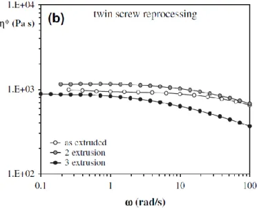
Another study by Darunee et al.[75] based on Polycarbonate (PC)/multi-walled carbon nanotubes. Figure 4.2 shows the storage and loss modulus and the complex viscosity at different injection molding cycles processed at 260°C. The G′ and G′′ of the PC/MWCNT composites show a tendency to decrease with increasing injection molding cycles. It is clear that G′ and G′′ increased with increasing the frequency for all injection molding cycles. It is suggested that the increase of rheological properties of the PC/ MWCNT composites at high frequency is related to an increase of the MWCNTMWCNT network structure because of low degree of aggregation of MWCNTs at high frequency. The rheological properties of polymer composites at high frequency region reflect the dynamics of polymer entanglement [75,76].

(43)

Figure 4.2: Effect of reprocessing on G’, G’’ and η*_{of the PC/MWCNT composites [75]}

A shear thinning behavior was observed for the η* of the PC/ MWCNT composites at different injection molding cycles. The shear-thinning behavior and longtime relaxation suggest a pseudo-solid-like behavior of the PC/MWCNT composites [75].

(44)

(45)

Chapter 3: Materials and methods

3.1 Materials and formulations

The polymer materials used in this study consist of Polyamide 66 (PA) Ultramid® A3W produced by BASF®. The basis of the product range are polyamides, supplied in a variety of molecular weights or viscosities, have a range of additives and are reinforced with glass fibers or minerals. These materials have become indispensable in almost all fields of engineering for the most varied components and high stressed machine parts (e.g. bearings, bearing cages, gear wheels coil formers etc.), as high-quality electrical insulating materials (e.g. cable connectors) and for many special applications. Table 1 summarizes the most relevant properties of BASFs Ultramid ® A3W.

Table 1: Most relevant properties od Ultramid® A3W

1

Material Polyamide 66 (Ultramid®)

Supplier BASF®

Grade A3W

Density 1130 kg/m3

MVR 275°C/5kg 100 cm3_/10min

Extended information on the A3W grade Ultramid® material can be found in the Appendix A.

Two types of graphene nanoparticles were used in the production of the nanocomposites. It is known that they differ in terms of particle size. Thus, the designations used for the graphene nanoparticles was EG (Graphene 2) and GnP (Graphene 1), corresponding to the larger and smaller nanoparticle size, respectively. Coding of the materials was done by the supplier (BASF®).

In total 9 different reference nanocomposites were prepared by extrusion process. Formulation 1, consisted of extruded neat Ultramid® A3W. All other formulations (2 to 8) are produced by addition of Graphene 1 or Graphene 2 to the neat polymer and by

(46)

combining different processing conditions. In all formulations added, graphene was at 7% wt. Table 2 provides the composition of the nanocomposite materials prepared in this work in terms weight percentages.

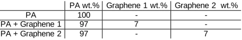
Table 2: Formulations used in this work in terms of weight percentages 2

PA wt.% Graphene 1 wt.% Graphene 2 wt.%

PA 100 - -

PA + Graphene 1 97 7 -

PA + Graphene 2 97 - 7

Finally, all the possible formulations in terms of graphene type used are provided in Table 3.

Table 3: All formulations in terms of graphene type 3

Formulation Materials

1 Neat PA (A3W, Ultramid®) 2 PA + Graphene 1 (smaller) 3 PA + Graphene 1 (smaller) 4 PA + Graphene 1 (smaller) 5 PA + Graphene 1 (smaller) 6 PA + Graphene 2 (larger) 7 PA + Graphene 2 (larger) 8 PA + Graphene 2 (larger) 9 PA + Graphene 2 (larger)

(47)

3.2 Nanocomposite preparation and sample acquisition

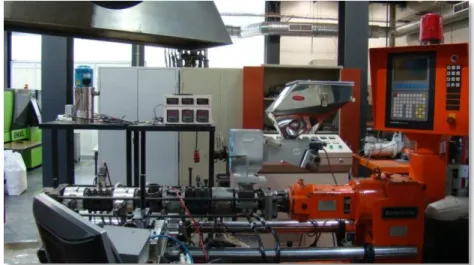
Nanocomposites were produced via extrusion compounding by means of Leistritz LSM 30.34 modular co-rotating inter-meshing twin-screw extruder. Figure 5 shows an actual picture of the machine. The polymer pallets were fed into the extruder at a constant throughput rate using volumetric feeder located upstream at the initial section of the extruder barrel. The graphene filler was introduced in the extruder by a side feeder after polymer melting stage (zone 4). Additionally, sections of the extruder barrel were modified in order to accommodate rotary valves used for collecting molten samples at specific locations along the process line. Figure 6 shows the extruder barrel and screw configurations, as the relative distances along the axial length of the extruder. Notice that the barrel units housing the rotary valves were placed at zones 3, 5 and 7.

According to the screw configuration used, these zones coincide with the kneading block sections where melting (zone 3) and most of the mixing takes place (zones 5 and 7). All the collection points (L/D=15,17,24) were carefully chosen. First collection point (L/D=15) was selected in order to get an insight what is happening inside the extruder before any of the mixing took place. While second and third collection points (L/D=17,24) are used to depict the material after second (L/D=17) and third (L/D=24 ) kneading blocks.

Note that immediately after the second and third kneading block (zone 5 and 7) there is a left-handed section that provides positive pressure for the collection of the material and also retains material in the kneading blocks facilitating better intensive mixing. The evaluation of the nanocomposite dispersion due to production parameters requires the use of different sets of processing conditions. Table 4 reports the processing conditions used for the production of the nanocomposite samples.

It has to be noted that this project was supported by BASF® and of the processing conditions (screw profile, temperature, feed rate, screw speed) and materials used were set and provided by BASF®. Figur e 5

(48)

Figure 5. Leistritz LSM 30.34 in the polymer processing laboratory of University of Minho, Portugal Figur e 6

1

Figure 6. Screw profile with extruder barrel setup Table 4: Processing conditions

4

Condition Throughput rate (kg/h) Screw speed (rpm) Barrel temperature (ºC) 1 9 200 280 2 9 300 3 15 200 4 15 300

1_{Where, xxRy and xxRyL are right-handed and left-handed conveying elements. with xx being the pitch in}

millimeters and R(=120)/y is the screw element length. xxKBy represents a kneading block with xx being the number of kneading disks and y, the staggering angle, is given in degrees.

(49)

Samples for off-line characterization were collected at axial locations L/D 15, 17, 24 – corresponding to the beginning of the first mixing zone, end of the first mixing zone, and midway of the second mixing zone respectively (see Fig. 6). Collection of the samples was performed only after the process reached its steady state.

(50)

3.3 Sample preparation

3.3.1 Rheology samples

Disk-shaped specimens were produced via compression molding from the samples collected along the extruder. Since polyamides are known to exhibit hydrophilic features, the samples were conditioned at 100°C for 1h in a Binder® FD heating oven in order to remove any excess moisture prior to compression molding.

Material collection was done manually and consequently the obtained material samples were mainly bulky and roughly shaped upon solidification. To enhance the drying process and simplify disk preparation material was cut into smallest possible pieces with scissor cutter. The mold used to shape the disks consisted of a steel frame with 9 identical openings (see Fig. 7). Each of the openings was φ25mm in diameter and 1mm in thickness. Mold openings were manually filled with approximately same amount of material on the North (N), South (S), West (W) and East (E) openings. In turn, North East (NE), North West (NW), South East (SE) and South West (SW) openings were left intentionally empty. The reason behind why not all openings were filled is because there was a need to assure that all samples experience the same pressure during compression molding. Teflon® foils were inserted between the mold and the supporting metal plates in order to prevent sticking of the samples to the metallic parts. Compression molding of the samples was possible by means of a Moore® 50 tons hydraulic press. The flowchart below summarizes the steps of the molding cycle:

Molding temperature Tmo= 300°C

Accommodation time t = 1min. at 30t Molding time t = 5min. at 45t

Water cooling

(51)

The molding temperature was set 20°C above the melting temperature of the material (Tm=280°C) in order to ensure that the polymer is completely molten and have a

viscosity which facilitates its shaping. After 5 minutes of molding, disks were water cooled while under pressure and demolding was done when the temperature reached Td=240°C.

Figur e 7

Figure 7. Disk mold with the final sample on the left

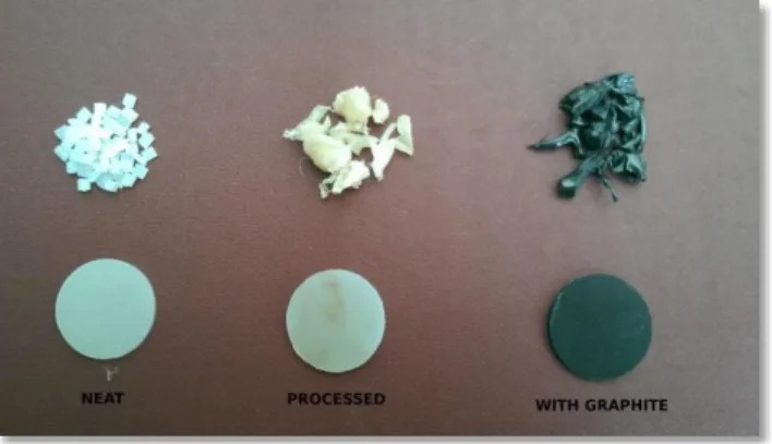
Figure 8 depicts the final look of the disks with corresponding palletized material utilized for their production. It has to be noted that there are changes in color between processed and neat PA that could indicate degradation.

Figur e 8

Figure 8. Material from which the disks were made and their final shape after molding. From left to right, neat (Ultramid®), processed

(52)

3.3.2 Optical microscopy samples

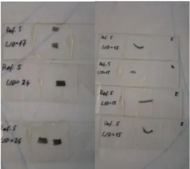
Samples for optical microscopy characterization were cut with Leitz® 1401 microtome (see Fig. 9), using glass knives, to a thickness of 4µm. The samples were then embedded in Canadian balsam between the lamina and lamella, and left for 24h to settle and dry (see Fig. 10).

Figur e 9

Figure 9: Leitz® 1401 microtome (left) and glass cutter (right)

Figur e 10

(53)

3.4 Characterization techniques

3.4.1 Rheology

The rheological characterization of the samples collected along the extruder was performed with a TA Instruments AR-G2® rheometer set to small amplitude oscillatory shear experiments (SAOS) using parallel plate geometry. Figure 11 shows the rheometer used. Experiments were done with a measuring plate of φ25mm in diameter, a distance between the plates of 0.9mm and a set temperature of 280°C. Samples were subjected to 2min waiting time for thermal homogenization before start the test. In order to ensure that there was no buildup of water content from the environment, all the disks were dried for 1h at 100°C in the Binder® heating oven before placing them inside the rheometer. Note that AR-G2 rheometer is equipped with an internal monitoring camera and that some samples exhibited bubbling of air when heated to the measuring temperature (T=280°C). Possible explanation lies in the fact that some could get trapped in the compression molding process.

Figur e 11

Figure 11: AR-G2 rheometer

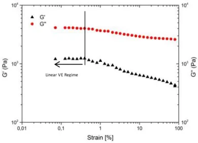
A suitable strain value within the linear viscoelastic range of the nanocomposites was assessed through a dynamic strain amplitude experiment. The results are shown in

(54)

Figure 12 indicate that at strain values up to 0.3% the viscoelastic moduli are maintained constant, corresponding to the linear regime of the material. Thus, the strain magnitude chosen for the SAOS experiments was 0.3%.

Figur e 12

Figure 12. Linear viscoelastic regimes based on Formulation 5 samples

3.4.2 Optical microscopy

Microscopy analysis was performed with an Olympus® BH-2 microscope (see Fig. 13, left) set to a magnification of 4x and 20x, corresponding to a general and detailed view of the samples, respectively. A Leica® DFC 280 video camera (see Fig. 13, right) and corresponding software (see Fig. 13, center) were used in order to register the micrographs resulting from the analysis.

Figur e 13

(55)

3.5 Data processing

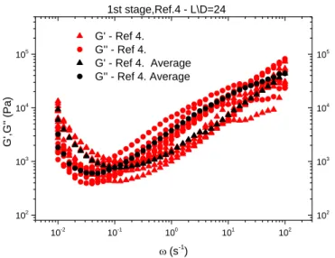
In order to properly analyze and draw relevant conclusions from the measurements, first all the measured data had to be systematically post processed and treated with the exact same procedures. As an example, Formulation 4 processed with condition 3, was selected to depict the distinct stages the raw data was subjected to. Although, measurement for some formulations were repeated for as much as 8 or 9 times in many cases only two data sets could be considered valid and used for further data processing. In the first stage, all the collected data points were plotted and the average line (first) was calculated from all the measurement repetitions and placed in to the same graph (see Fig. 14).Figur e 14

10-2 10-1 100 101 102 102 103 104 105 102 103 104 105 G' - Ref 4. G'' - Ref 4. G' - Ref 4. Average G'' - Ref 4. Average G',G '' ( Pa) 1st stage,Ref.4 - L\D=24 (s-1₎

Figure 14. First stage in data processing of Formulation 4, L/D=24 (G’, G’’)

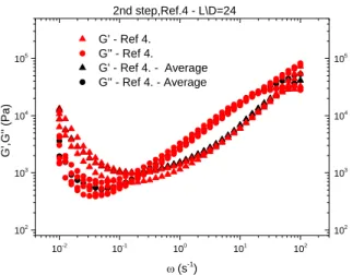
In the second stage, the outlier curves were visually assessed and the ones that deviated the most from the previously calculated average lines were removed and their values were not used in further calculations. After the removal of the mentioned curves, new (second) average lines were calculated from the remaining measurements (see Fig. 15).

(56)

10-2 10-1 100 101 102 102 103 104 105 102 103 104 105 G' - Ref 4. G'' - Ref 4. G' - Ref 4. - Average G'' - Ref 4. - Average G',G '' ( Pa) 2nd step,Ref.4 - L\D=24 (s-1 )

Figure 15. Second stage in data processing of Formulation 4, L/D=24 (G’, G’’)

In the third stage, individual measurement points that deviated extremely from the calculated second average curves were removed. The removal of individual data points was judged based on the diagrams of dissipation factor tan δ (see Fig. 16). As can be seen from the Figure 16, oscillations in measured values can be easily observed and problematic data points (encircled in red) singled out and removed. Problematic points were attributed to the experimental errors due to some bubbles being entrapped in the sample. In order to prove this assumption, further measurements are needed. Loss tangent (tan δ) was calculated by the following equation:

0,01 0,1 1 10 100 0,1 1 10-1 100 tan d 3rd step,Ref.4 - L\D=24, tan d (s-1 )

(57)

It has to be noted that there was no pre shearing prior to the rheological measurements since it could easily affect the existing dispersion state of the samples [72]. It is speculated that, since the disks have been at rest it allowed for a partial particle reagglomeration. As shown by the behavior of the moduli at low frequency range (between 0,01 s-1_{and 0,05s}-1_{) material is crosslinking (see Fig. 14,15) and this is}

contributed to the thermal degradation. Similar behavior was reported by Han et al. [73] and Lozano-Gonzales [74]. Taking these assumptions into consideration the final look of the curves is given on the Figure 17.

10-1 100 101 102 102 103 104 105 102 103 104 105 G' ( Pa) PA + Graphene 1 (Ref.4) G' - Ref.4 and 8- average, Feed rate=15, Screw speed=200

(s-1)

(58)

(59)

Chapter 4: Results and discussion

4.1 Effect of presence and type of graphene

In this subsection we will present the effects of different graphene types on the viscoelastic properties of the nanocomposites. All the material references used have undergone the same processing conditions (Condition 1 – throughput = 9 kg/h and screw speed = 200 rpm).

In the first case, formulations 1, 2 and 6 will be studied and compared. Figure 18 and Figure 19 show the comparison of the moduli and the complex viscosity of neat material Formulation 1 (PA), Formulation 2 (PA + Graphene 1(smaller)) and Formulation 6 (PA + Graphene 2(larger)). 10-1 ₁₀0 ₁₀1 ₁₀2 102 103 104 105 102 103 104 105 G' ( Pa)

G' - Form.1,2,6 - average, Feed rate=9, Screw speed=200 Form.1 - PA (neat)

Form.2 - PA + Graphene 1 (smaller) Form.6 - PA + Graphene 2 (bigger)

(s-1₎ 10-1 ₁₀0 ₁₀1 ₁₀2 102 103 104 105 102 103 104 105 Form.1 - PA (neat)

Form.2 - PA + Graphene 1 (smaller) Form.6 - PA + Graphene 2 (bigger)

G''

(Pa)

G'' - Form.1,2,6 - average, Feed rate=9, Screw speed=200

(s-1₎

Figure 18. Comparison of storage modulus G’ (left) and loss modulus G’’ (right) for formulations 1, 2 and 6

The introduction of graphene enhances the magnitude of the viscoelastic properties and leads to an absence of the Newtonian plateau region at lower frequency values (from 10 -1_{to 1s}-1_{). Also, a faster drop in viscosity is evident. This was also observed in a study of}

Russo et al. [72]. In addition the slopes of the composite materials are similar and the steepness is less pronounced in comparison to the neat (Ultramid®) material.

(60)

10-1 100 101 102 102 103 104 105 102 103 104 105 Form.1 - PA (neat)

Form.2 - PA + Graphene 1 (smaller) Form.6 - PA + Graphene 2 (larger)

h - Form.1,2,6 - average, Feed rate=9, Screw speed=200

|



 | (Pa.s)

(s-1)

Figure 19. Comparison of η, for formulation 1, 2 and 6

In the second case, formulations 5 (PA + Graphene 1(smaller)) and 9 (PA + Graphene 2(larger)) as well as 4 (PA + Graphene 1(smaller)) and 8 (PA + Graphene 2(larger)) will be compared, respectively. Processing conditions used were Condition 3 (Formulations 4 and 8) and Condition 4 (Formulations 5 and 9). Note that the main difference is also in graphene particle size while the processing conditions are kept constant.

It has to be noted that the initial difference in G’ is much higher at the low frequency range in comparison to the high frequencies. At the higher frequencies the values of G’ come together for formulation 5 and 9 (see Fig. 20a) and the same kind of behavior can be observed for formulations 4 and 8 as well (Figure20b). It is understood that at the lower frequency level measurements are more sensitive to the probing of dispersion levels and that increase of frequency induces a more dominant hydrodynamic flow which in turn reduces the sensitivity for material structure. In two studies by D. Aussawasathien et al. [75,76] the same conclusions were drown.

(61)

10-1 100 101 102 103 101 102 103 104 105 106 101 102 103 104 105 106 G' ( Pa)

G' - Form.5 and 9- average, Feed rate=15, Screw speed=300

(s-1 ) 10-1 100 101 102 102 103 104 105 102 103 104 105 G' ( Pa)

G' - Form.4 and 8- average, Feed rate=15, Screw speed=200

(s-1

)

Figure 20. Comparison of storage modulus G’ for a)Formulations 5 and 9 and b) Formulations 4 and 8

10-1 ₁₀0 ₁₀1 ₁₀2 102 103 104 105 102 103 104 105 Form.5 - PA + Graphene 1 (smaller)

Form.9 - PA + Graphene 2 (larger)

h - Form.5 and 9- average, Feed rate=15, Screw speed=300

|  | (Pa.s) (s-1₎ 10-2 ₁₀-1 ₁₀0 ₁₀1 ₁₀2 102 103 104 105 102 103 104 105 Form.4 - PA + Graphene 1 (smaller) Form.8 - PA + Graphene 2 (larger) h - Form.4 and 8- average, Feed rate=15, Screw speed=200

|



| (Pa.s)

(s-1₎

Figure 21. Comparison of η* for c)formulation 5 and 9 and d) formulation 4 and 8

The increase in G’, G’’ and η* is a clear indication that when the processing conditions are kept constant and the nanocomposite formulation is being varied (by addition of Graphene 1 or 2) better dispersion levels are achieved with smaller graphene filler - Graphene 1.

(62)

4.2 Effect of the feed rate

Study of the effects of feed rate will be done on two sets of references. First, Formulation 2 (PA + Graphene 1(smaller)) and 4 (PA + Graphene 1(smaller)) will be compared followed by the comparison of 6 (PA + Graphene 2(larger)) and 8 (PA + Graphene 2(larger)) formulations. Processing conditions used were Condition 1 (Formulations 2 and 6) and Condition 3 (Formulations 4 and 8). Note that the main difference that sets comparison pairs apart is the feed rate (9/15 kg/h) while the screw speed was kept constant (200 rpm).

Formulations 2 and 4 both feature smaller Graphene 1. Figure 22 presents G’ and G’’ comparatively for both nanocomposite materials while the comparison of complex viscosity is given on the Figure 23.

10-1 100 101 102 102 103 104 105 102 103 104 105 G' ( Pa)

Form.2 - PA + Graphene 1 (smaller), 9kg/h From.4 - PA + Graphene 1 (smaller), 15kg/h G' - Form.2 and 4- average, Feed rate=9,15 Screw speed=200

(s-1 ) 10-1 100 101 102 102 103 104 105 102 103 104 105 Form.2 - PA + Graphene 1 (smaller), 9kg/h From.4 - PA + Graphene 1 (smaller), 15kg/h G'' - Form.2 and 4- average, Feed rate=9,15 Screw speed=200

G''

(Pa)

(s-1

)

Figure 22. Comparison of formulation 2 and 4 for a)G’ and b) G’’

As can be observed from abowe graphs (see Fig. 22), only influence of different feed rates is higher values of G’ at lower frequencies. The same kind of behavior corresponds to viscosity, as can be seen on below graph (see Fig. 23).

(63)

10-1 ₁₀0 ₁₀1 ₁₀2 102 103 104 105 102 103 104 105

Form.2 - PA + Graphene 1 (smaller), 9kg/h From.4 - PA + Graphene 1 (smaller), 15kg/h h - Form.2 and 4- average, Feed rate=9,15 Screw speed=200

|



| (Pa.s)

(s-1

)

Figure 23. Comparison of complex viscosities for formulation 2 and 4

Second set of comparrison formulation consists of data from formulations 6 and 8. In this case both formulations are derived with larger Graphene 2. Comparison of G’ and G’’ is depicted on Figure 24 and for the complex viscosity on Figure 25.

10-1 100 101 102 102 103 104 105 102 103 104 105 G' ( Pa)

Form.6 - PA + Graphene 2 (larger), 9kg/h Form.8 - PA + Graphene 2 (larger), 15kg/h G' - Form.6 and 8- average, Feed rate=9,15, Screw speed=200

(s-1 ) 10-1 100 101 102 102 103 104 105 102 103 104 105 Form.6 - PA + Graphene 2 (larger), 9kg/h Form.8 - PA + Graphene 2 (larger), 15kg/h G'' - Form.6 and 8- average, Feed rate=9,15, Screw speed=200

G''

(Pa)

(s-1

)