ALGORITHMS FOR EXTERNAL TRACKING OF AN AUV1
An´ıbal Matos, Nuno Cruz
Faculdade de Engenharia da Universidade do Porto Instituto de Sistemas e Rob´otica – Porto
R. Dr. Roberto Frias 4200-465 Porto Portugal
{anibal, nacruz}@fe.up.pt
Abstract: In this paper we describe the algorithms used in the external tracking system of the Isurus AUV. By listening to the acoustic signals exchanged between the vehicle and the beacons of the acoustic navigation network, the tracking system is able to obtain distance measurements from the vehicle to each beacon, that are then used to compute the vehicle horizontal position. Several error sources make these measurements inadequate to be used for computing the vehicle position by a simple triangulation technique. The tracking algorithms described here are able to reject highly erroneous measurements, producing position estimates with a satisfactory degree of accuracy. Copyright c° 2004 IFAC
Keywords: Autonomous Underwater Vehicles, Navigation, Tracking.
1. INTRODUCTION
The number of successful missions with au-tonomous underwater vehicles (AUVs) has been increasing steadily during the last few years, val-idating this emerging technology as an efficient tool for underwater sampling. Nonetheless, there is always the risk of loosing an AUV while per-forming autonomous missions. This risk can be greatly reduced if the progress of the vehicle op-eration is monitored so that anomalous behaviors can be readily detected and recovery measures can be taken in due time.
Although most AUVs operate without any com-munication link, it is still possible to monitor the vehicle operation just by externally tracking the position of the vehicle in real time. This kind of monitoring, though quite simple, can be very
1 Supported by POCTI, POSI and DEEC/FEUP
effective in detecting major troubles and avoid-ing vehicle losses since most vehicle malfunctions result in deviations of the vehicle from the pre-scribed trajectory.
In this paper with describe the algorithms used in the external tracking of the Isurus AUV. This is a small size AUV that is being operated for the last 6 years by the Underwater Systems and Technol-ogy Lab (LSTS) of the University of Porto. The paper is organized as follows. In section 2 we describe the Isurus AUV and give an overview of the operational mission performed with this vehicle over the last years. In section 3 we detail the acoustic navigation system of this vehicle paying more interest on the issues that enable the external tracking. Section 4 is devoted to the principles of operation and to the architecture of the external tracking system. Section 5 describes in detail the models and algorithms used in the
Fig. 1. The Isurus AUV.
tracking system, as well as some experimental results.
2. THE ISURUS AUV
Isurus (Fig. 1) is a REMUS class AUV, built by the Woods Hole Oceanographic Institution, MA, USA, in 1997. These vehicles are low cost, lightweight AUVs specially designed for coastal waters monitoring (von Alt et al., 1994). The reduced weight and dimensions makes them ex-tremely easy to handle, requiring no special equip-ment for launching and recovering. Isurus has a diameter of 20 cm and is about 1.5 meters long, weighting about 35 kg in air. Inside the hull sev-eral subsystems have been improved or specifi-cally developed at LSTS, contributing to the con-tinuous enhancement of the vehicle performance and reliability. The maximum forward speed of the vehicle is 4 knots, however the best energy efficiency is achieved at about 2 knots. At this velocity, the energy provided by the rechargeable Lithium-Ion batteries lasts for over 20 hours (i.e., over 40 miles). Although small in size, it is possible to accommodate a wide range of oceanographic sensors, according to mission objectives. For the missions already performed, we have integrated a CTD and an altimeter in a specially designed nose extension. Successful tests have also been performed in the past with sidescan sonars, ADCP (Acoustic Doppler Current Profiler), and Optical BackScatter.
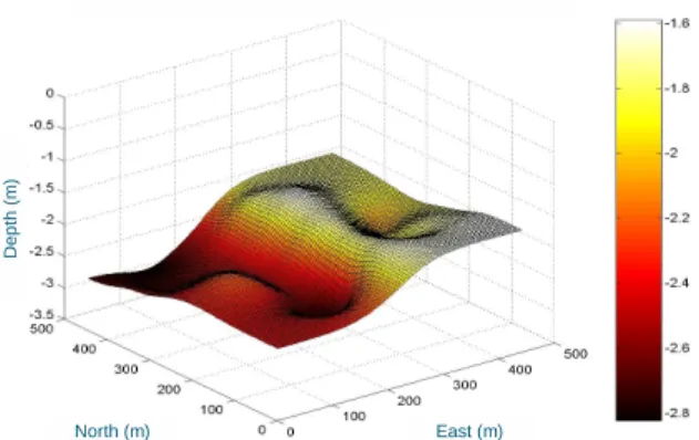
The first operational missions with Isurus took place in 1998, in the estuary of the river Minho, in the northern border between Portugal and Spain. During autonomous missions, typically longer than one hour, the vehicle continuously collected CTD and bathymetric data, while navigating on an acoustic network. At the end of each mission, the vehicle was recovered and data was uploaded to a laptop computer for display and validation. As an example, Fig. 2 shows a bathymetric map of the river estuary, generated by the post processing of a mission data.
During the missions in the river Minho, the vehi-cle and the acoustic transponders were deployed and recovered by 2 people from a small fishing boat, which demonstrated the reliability and the operational effectiveness of the system (Cruz et
D e p th ( m ) North (m) East (m)
Fig. 2. Bathymetric data.
al., 1999). Since then, several other similar
mis-sions have been performed on different scenar-ios. One example was the evaluation of the en-vironmental impact of the heated discharge of a power plant located near the Crestuma dam in the river Douro. This included the influence in the mixing process of the river bed, the free surface and the interaction with bottom topography. For this analysis, the AUV was programmed to collect CTD data near the discharge outfall as well as bathymetric data (Ramos et al., 2000).
3. NAVIGATION SYSTEM
The position of the Isurus AUV is estimated in real time from data provided by several devices and systems. The vehicle depth is directly ob-tained by a depth pressure cell installed on the vehicle. The vehicle horizontal position is obtained from dead reckoning and absolute positioning data. The dead reckoning data is composed by the vehicle attitude, obtained from a digital compass and a set of tilt sensors, and also by the vehicle velocity with respect to the water, obtained from an encoder that measures the propeller rotation speed. The absolute positioning is obtained from a long baseline navigation network. The network is composed by acoustic beacons that are deployed in the operation area. During the mission, the vehicle interrogates the beacons to determine the distance to each of them. With at least 2 beacons located in different places, it is then possible to determine the position of the vehicle, assuming it does not cross the vertical plane joining the 2 beacons.
The horizontal position of the vehicle is estimated in real time by fusing together distance measure-ments with dead reckoning data using an extended Kalman filter (Matos et al., 1999). This filter is based on a simple model of the vehicle motion that takes into account the velocity of the vehicle with respect to the water as well as the velocity of the water mass. The navigation data is logged by the vehicle onboard computer and is used after the
Fig. 3. Acoustic beacon.
mission completion to further improve the accu-racy of the position estimates (Matos et al., 2003). The beacons used in the navigation network (Fig. 3) are multi-frequency transponders and were developed at the LSTS (Cruz et al., 2001). Each beacon can be configured to reply with a signal of a given frequency when interrogated by another signal of a different frequency.
While navigating, the vehicle onboard software completely controls the exchange of acoustic sig-nals and obtains the range measurements one at a time. To determine its range to a given beacon, the vehicle first sends an interrogation signal. All the beacons detect that signal but only the one identified with such interrogation signal will reply with signal of a predefined frequency. Upon detec-tion of the beacon reply, the vehicle measures the elapse time, computes the range, and interrogates another beacon, starting a new range measure-ment.
4. EXTERNAL TRACKING SYSTEM The external tracking of the Isurus AUV can be accomplished just by listening to the acoustic sig-nals exchanged between the vehicle and the nav-igation beacons and relies on a simple algorithm that was proposed in (Cruz et al., 2001).
To illustrate the tracking mechanism let us con-sider that the AUV is using beacons A and B to navigate. Under normal operation, the vehicle will transmit frequency fA to interrogate beacon A and wait for the reply signal. As soon as this
reply is detected, it will transmit frequency fB to interrogate beacon B and wait for the reply from this beacons. This sequence will proceed through-out the mission. Any listening device tapping the acoustic channel will detect all transmissions. The time elapsed between the detection of frequency
fA and the detection of fB corresponds to twice the range between the vehicle and transponder
Fig. 4. Surface buoy.
A; the time elapsed between the detection of
frequency fB and the detection of frequency fB corresponds to twice the range between the vehicle and transponder B. Providing that the listening device is within acoustic range to the vehicles, this mechanism works independently of the location, as it only deals with time differences.
To be precise, the vehicle only emits the interro-gation signal to a beacon a given delay (typically less than 2 seconds) after receiving the reply from the previous beacon in the interrogation sequence. The main reason for this delay to exist is to avoid interactions between signals from different interrogation cycles. In fact, almost all acoustic signals give rise to multiple reflected signals at the boundaries of the water mass. The presence of such signals extends well beyond the intended lifespan of the original one, but their amplitudes decay with time. It is therefore necessary to wait a certain time (this time depends mainly on the environment where the mission is taking place) before emitting a signal of a frequency used before, to avoid erroneous signal detections. Since this delay is preprogrammed in the vehicle onboard software, it can be properly accounted for when tracking the vehicle externally. In practice, it only affects the performance of the tracking system (and also of the onboard navigation system) by lowering the rate at which new range measure-ments become available.
The Isurus tracking system is composed by a LSTS multi-frequency transponder acting as the listening device, a communication link and a per-sonal computer. Even if the tracking mechanism works with a non stationary listening device, it is usual to have it moored and connected to a surface buoy (Fig. 4). The listening device sends a time stamped message whenever it detects a new acoustic signal. The buoy is equipped with a radio modem and retransmits the data received from the listening device to the personal computer. The computer processes the messages sent by the
lis-Fig. 5. Tracking software.
tening device, estimates the position of the vehicle and displays it in a graphical interface (Fig. 5). Although the tracking mechanism described above is very straightforward, the range measurements obtained in such a way cannot be used to compute the vehicle horizontal position by a simple trian-gulation algorithm. In fact, the range measure-ments are subject to errors from different sources, namely,
sound speed: the velocity of sound varies from place to place according to the characteristics of the water mass (mainly temperature and density) and is considered to be constant; multipath propagation: the acoustic wave is
subject to multiple reflections at the boundaries of the water mass (surface, bottom, submerged structures) resulting in non direct propagations between emitter and receiver as required for range computation;
vehicle motion: since the vehicle is moving, its distances to acoustic beacons and tracking de-vice change with time, introducing errors in the tracking mechanism;
non deterministic delays: the delay between the detection of a beacon reply by the vehicle and the emission of a new interrogation signal depends on the onboard processor response time and can be subject to variations of a few milliseconds; this information is not available outside the vehicle and therefore introduces further errors in the tracking mechanism; vehicle depth: the vehicle depth is not known
externally, so the corrections due to depth dif-ferences between vehicle and beacons cannot be taken into account.
5. TRACKING ALGORITHMS
The basis of the tracking system is the beacon interrogation and reply sequence described above. To further understand how the distances between the vehicle and the beacons are computed and how the different error sources enter in the measure-ments let us consider an interrogation cycle. At
a given time t0 the vehicle emits an interrogation signal to a beacon, say A. This signal propagates through the water and at time tA is detected by beacon A. It is also detected by the tracking device at tiT. A predefined delay, δA, after tAthe beacon A emits its reply signal. This signal is then detected by the vehicle at time tV and by the tracking device at trT. At time tn = tV + δV the vehicle initiates another cycle, emitting an interro-gation signal to another beacon, say B. This signal is detected by the tracking device at tnT. The tracking device has a clock and is therefore able to measure the differences trT− tiT and tnT− tiT. Let rAand rT be the distances from the vehicle to beacon A and to the tracking device, respectively, at time t0. Assuming a constant speed of sound in water, c, and straight line propagation of acoustic signals, we have
tA= t0+rA c tiT = t0+rT
c
It is also possible to write
tV = tA+ δA+ ¯ rA c trT = tA+ δA+ l c
where ¯rA is the distance between the vehicle and beacon A at time tV and l is the distance between beacon A and the tracking device at time trT. Finally, we can write
tnT = tn+ ¯
rT c
where ¯rT is the distance from the vehicle to the tracking device at tn. It will be useful to consider the values ∆A = ¯rA − rA and ∆T = ¯rT − rT that represent how much the vehicle travels away from beacon A in the interval [t0, tV] and from the tracking device in interval [t0, tn], respectively.
5.1 Measurements
The basic tracking mechanism uses the difference
tnT−tiT to estimate the distance from the vehicle to beacon A. Using the notation introduced above, we have
tnT − tiT = 2rA+ ∆A+ ∆T
c + δA+ δV.
In this equation, the difference tnT − tiT is ob-tained from the tracking device clock and the delays δA and δV are known a priori to a certain accuracy. The travelled distances ∆A and ∆T are not known or even measurable and have to be estimated based on a model for the motion of the vehicle. In the simplest case, these values can be taken as zero, meaning that the vehicle does not move significantly during the respective intervals.
The difference trT − tiT is just given by trT − tiT = rA− rT + l
c + δA.
Assuming that the distance between beacon A and the tracking device, l, is known, as is certainly the case when the listening device is located at a fixed place, this equation can be used to estimate the difference rA− rT, based on the time difference trT − tiT, also measured by the tracking device. These extra measurements will be referred to as
extended tracking.
5.2 Vehicle motion
As mentioned above, one has to consider a model for the vehicle motion to be able to estimate the correction terms ∆A and ∆T when computing the distance rAbased on the measurement tnT − tiT. This model is even more important if one notes that not all acoustic signals will be properly detected by the tracking device. Since each new range measurement will require two consecutive successful detections, the time interval between two new range measurements can be sometimes quite large. In those cases, it will be mandatory to predict how the vehicle position will evolve on such large intervals of time.
It is not desirable to have a complex model for the vehicle motion. In fact, the measurements obtainable from the data provided by the tracking device are just distances between the vehicle and the navigation beacons, and differences between those distances and the distance from the vehicle to the tracking device, in the case of extended
tracking.
During a typical mission, and for most of the time, the AUV will be moving along straight lines at a pretty constant speed. It is therefore reasonable to model the vehicle motion by a simple dynamic system that captures such behavior. The vehicle motion will then be modelled by the stochastic differential equation ˙x ˙vx ˙y ˙vy = 0 1 0 0 0 −β 0 0 0 0 0 1 0 0 0 −β x vx y vx + nx nvx ny nvy .
In this equation, (x, y) are the coordinates of the vehicle in the horizontal plane, and (vx, vy) are the horizontal components of the vehicle velocity, with respect to a fixed frame. The positive parameter
β models an exponential decay in the vehicle
velocity. The independent white noise processes
nx, nvx, nyand nvy, model the difference between the actual motion of the vehicle and the motion predicted by the deterministic part of this model.
5.3 Estimation algorithm
The remote tracking of the Isurus AUV consists in estimating, in real time, the evolution of the state of the dynamic system that models the vehicle motion, based on the measurements provided by the tracking device. This estimation is performed by an algorithm that uses an extend Kalman filter (Gelb et al., 1996). The filter data consists in the estimate of the state of the dynamic model and in the covariance matrix of the estimation errors. Let X− be the estimate of the vehicle state at time t0, when the vehicle sends an interrogation signal to a given beacon A, and let P−be the error covariance matrix at the same instant of time. In the extended tracking case, the next available measurement is the time difference ze = trT − tiT, and then the time difference zs = tnT − tiT. In the simple tracking case, the only available measurement is zs. These measurements are used to update the state and the covariance matrix to their new values X+ and P+.
To treat both the simple and extended track-ing similarly, consider the intermediate values Xi and Pi, of state and covariance matrix. For the simple tracking, we have simply Xi = X− and Pi= P−. For the extended tracking, these values are obtained from the Kalman filter correction relationships
Xi= X−+ Ke(ze− ze∗) Pi= P−− KeHeP− where z∗
e is the expected value of the time differ-ence trT− tiT, H is given by
He= ∂(trT − tiT) ∂X ¯¯¯
X=X−
and Ke = P−HeTSe−1, is the Kalman gain, Se= HeP−HeT + re, and re is the covariance of the error associated to the measurement of ze. To eliminate spurious measured data, the state and covariance values are updated only if the measure-ments satisfy kze−z∗ekS−1
e ≤ γ, where γ is a design
parameter.
The measurement zsis then used to compute X+ and P+, according to X+= Xi+ K s(zs− zs∗) P+= Pi− K sHsPi where z∗
s is the expected value of the time differ-ence tnT − tiT, Hs is given by Hs=∂(tnT − tiT) ∂X ¯¯¯ X=Xi and Ks= PiHsT £ HsPiHT + rs ¤−1 , is the Kalman gain, where rsis the covariance of the error asso-ciated to the measurement of zs. A measurement
−160 −140 −120 −100 −80 −60 −40 −20 0 −20 0 20 40 60 80 100 120 140 160 East (m) North (m)
Fig. 6. Simple tracking.
validation test, similar to the one presented above, is also used here to eliminate spurious measured data.
After the correction update mechanism, the esti-mate of the state and the covariance matrix, Xn and Pn, at the following interrogation time, t
n, are computed from X+ and Pn, according to
Xn= eAτX+ Pn= eAτ µ P++ Z τ 0 e−AsQe−ATs ds ¶ eATτ
where τ = tn− t0, Q = diag(qx, qvx, qy, qvy), and qx, qvx, qyand qvyare the covariances of the white noise processes driving the stochastic differential equation.
5.4 Experimental results
The tracking system with the above described algorithms has already been successfully used in operational missions with the Isurus AUV. Fig-ures 6 and 7 present results obtained by the simple and extended tracking algorithms, which illustrate the performance of the tracking system.
In both cases, the solid line represents the post mission estimate of the vehicle trajectory obtained by the smoothing algorithm already mentioned (the accuracy of this estimate is around 2 me-ters). The dotted lines represent the results ob-tained in real time using both alternatives of the tracking algorithm. As expected, the extended tracking system performance is superior to the simple tracking. In both cases, the tracking so-lution is within 10 meters of the real trajectory when the vehicle is describing almost straight lines and within about 30 meters when the vehicle is turning. This kind of behavior is also expected, since the dynamic model describing the vehicle motion is much more accurate when the vehicle travels in a straight line than when it is turning around. −160 −140 −120 −100 −80 −60 −40 −20 0 −20 0 20 40 60 80 100 120 140 160 East (m) North (m)
Fig. 7. Extended tracking.
6. CONCLUSIONS AND FUTURE WORK The results already obtained show the efectiveness of the tracking system in monitoring the vehicle behavior. The performance of the system is in fact quite good for straight line motion. In the future, we intend to include in the system information about the expected trajectory of the vehicle in or-der to further improve the tracking performance.
REFERENCES
Cruz, N., A. Matos, A. Martins, J. Silva, D. San-tos, D. Boutov, D. Ferreira and F. Pereira (1999). Estuarine environment studies with Isurus, a REMUS class AUV. In: Proc. of the
MTS/IEEE Conf. Oceans’99. Seattle, WA,
USA.
Cruz, N., L. Madureira, A. Matos and F. Pereira (2001). A versatile acoustic beacon for navi-gation and remote tracking of multiple under-water vehicles. In: Proc. of the MTS/IEEE
Conf. Oceans’01. Honolulu, HI, USA.
Gelb, A., J. Kasper Jr., R. Nash Jr., C. Price and A. Sutherland Jr. (1996). Applied Optimal
Estimation. The MIT Press. Cambridge, MA,
USA.
Matos, A., N. Cruz, A. Martins and F. Pereira (1999). Development and implementation of a low-cost LBL navigation systems for an AUV. In: Proc. of the MTS/IEEE Conf. Oceans’99. Seattle, WA, USA.
Matos, A., N. Cruz and F. L. Pereira (2003). Post mission trajectory smoothing for the Isurus AUV. In: Proc. of the MTS/IEEE
Conf. Oceans’03. San Diego, CA, USA.
Ramos, P., M. Neves, N. Cruz and F. L. Pereira (2000). Outfall monitoring using au-tonomous underwater vehicles. In: Proc. of
the Int. Conf. Marine Wastewater Discharges MWWD’2000. G´enova, Italy.
von Alt, C., B. Allen, T. Austin and R. Stokey (1994). Remote environmental measuring units. In: Proc. of the IEEE Symp. on AUV