Analysis of OECD Countries Well-being through Statis Methodology

(1)

Analysis of OECD Countries Well-being

through Statis Methodology

by

Fabricio Javier Rivadeneira Zambrano

Master Thesis in Data Analytics - Modelling, Data Analysis and Decision

Support System

Thesis supervised by:

Professora Doutora Adelaide Maria de Sousa Figueiredo

Professora Doutora Fernanda Otília de Sousa Figueiredo

Faculdade de Economia

Universidade do Porto

2016

(2)

ii

Biographical Note

Fabricio Rivadeneira Zambrano was born on 14th of October 1975 and is a native of Chone, city of province of Manabí, Ecuador. He finished the secondary school in the mathematical-physics specialization, in Gonzalo Abad Grijalva Secondary school. He graduated in Systems Engineering at the Eloy Alfaro University in Ecuador, in 2005, and with a passion for Data Analysis, joined the Master’s Degree in Modeling, Data Analysis and Decision Support Systems in the School of Economics and Management of the University of Porto (FEP).

He works in the Faculty of Computer Science at the Eloy Alfaro University in Ecuador, since 2006 and complemented his education with other courses about Information Technology in India and USA. He speaks Spanish and has knowledge of English.

I feel that this Master in Portugal represents the opportunity to know more about Fatima and Medjugorje, a gift in my life given by God …

(3)

iii

Acknowledgements

Thank God, Thank Our Lady of Fatima and of Medjugorje.

I express my special thanks to my supervisors Prof. Dra. Adelaide Figueiredo and Prof. Dra. Fernanda Figueiredo for their time, patience, support, availability, suggestions and ideas, which were very important to the realization of this dissertation.

I want to thank to all my teachers in special, to Prof. Dr. João Gama for giving me their knowledge to improve me and to share in my country.

I express my special thanks to my mother and father and all my family in Ecuador for giving me their prayers to continue with my studies. Special thanks, to my wife Silvia, she helped me in difficult moments with all your love, to my sons, they shared with me a great part of my life.

I want to thank to all people of Erasmus Mundus Project, for giving me this opportunity to study this Master.

I want to thank to all my friends and colleagues, in Portugal and Ecuador, who have passed throughout my life and somehow have contributed to it.

(4)

iv

Abstract

In this thesis we aim to study the evolution of some developed countries and also of some emerging countries that are members of the OECD in what concerns some indicators (variables) of well-being during the period 2011-2015, through the STATIS methodology. This methodology allows to analyze the presence of a common structure in several data tables obtained over time, to identify the differences and similarities along the period of time under study and according to well-being indicators included in the OECD Your Better Life Index, and to analyze the trajectories of the countries.

Keywords: Principal Component Analysis, Statis Methodology, Three-way Data Methods, Well-being Indicators

(5)

v

Tables

Table 2.1. Names of data sets according to particular structure of data ... 7

Table 2.2. Basic techniques for analyzing a data table ... 8

Table 2.3. Original methods and obtained of original methods ... 8

Table 2.3. Original methods and obtained of original methods (cont.) ... 9

Table 3.1. The OECD Members countries and their ISO codes ... 19

Table 3.2. The indicators and a short description ... 20

Table 3.2. The indicators and a short description (cont.) ... 21

Table 3.2. The indicators and a short description (cont.) ... 22

Table 3.3. Descriptive statistics for 2011 ... 23

Table 4.1. Matrix of the RV coefficients ... 34

Table 4.2. Matrix of the Euclidean distances ... 34

Table 4.3. Eigenvalues, Inertia and Cumulative Inertia of the Interstructure ... 34

Table 4.4. Scalar products and distances to the compromise object ... 36

Table 4.5. Eigenvalues, Inertia and Cumulative Inertia of the first ten axes ... 36

Table 4.6. Decomposition of the sum of squared distances and decomposition of the squared distances ... 42

(7)

vii

Figures

Figure 2.1. General structure of three-way data sets ... 5

Figure 2.2. General structure of multi-block data tables ... 5

Figure 2.3. The different data tables of the years are put contiguous to each other ... 6

Figure 2.4. The different data tables of the years are put on a stack, whose columns are the same variables ... 6

Figure 2.5. The OECD well-being conceptual dimensions. Source: (OECD, 2013) ... 12

Figure 2.6. The screenshot of Your Better Life Index web application. The screenshot shows the BLI of countries displayed by rank (OECD, 2015) ... 13

Figure 3.1. The main steps of STATIS method ... 18

Figure 3.2. Boxplots of Material Conditions variables ... 29

Figure 3.3. Boxplots of Quality of Life variables ... 30

Figure 3.3. Boxplots of Quality of Life variables (cont.) ... 31

Figure 4.1. Centred Interstructure Euclidean Image ... 35

Figure 4.2. Countries’ compromise Euclidean image in the plan [1, 2] ... 37

Figure 4.8. Countries’ trajectories in the plan [1, 2] ... 44

(8)

1

CHAPTER 1 Introduction

This section contains the introductory aspects of the thesis, specifically the motivation for choosing the theme and the methodology used, the main proposed objectives for the construction of the complete analysis and the problem description to solve.

It also contains a brief reference to the thesis structure, synthesized by the description of the contents of each chapter.

1.1 Motivation

The process of analyzing data and how to manage that process is very relevant for today’s organizations as it can be applied to analyze and improve any type of operation in a variety of domains. Data analysis process leads us towards coherent and useful results.

Various data analysis techniques and algorithms can be used to learn the development of phenomena from raw data and they are very useful nowadays when there are a lot of data around us.

So, currently there are a special interest in the joint analysis of multiple data tables, named several multi-blocks or multi-way analysis. Most of these methods are extensions of Principal Component Analysis.

On the other hand, there is also a global interest in analyzing the well-being evolution of countries.

Thus, the methodology chosen in this thesis is STATIS (‘Structuration des Tableaux À Trois Indices de la Statistique’ in French or ‘Structuring Three-way data sets in Statistics’ in English), that is one of the main methods for developing other complex techniques of joint analysis of several data sets, and it is applied in the analysis of the Organisation for Economic Co-operation and Development (OECD) countries using well-being indicators.

(9)

2

1.2 Objectives

Through the joint analysis of multiple data tables using the STATIS methodology, this thesis proposes to analyze a set of tables used to calculate the Better Life Index in OECD countries, in order to know the performance of OECD countries, as well as their trends in the 2011-2015 period.

For that, we used several tables, where each table contains a set of well-being indicators of the OECD countries for a specific year, those indicators represent key factors, like housing, income, jobs, community, education, environment, civic engagement, health, life satisfaction, safety, work-life balance. So these eleven topics of the index are currently based on one to four indicators.

Thereby, the main objective of this dissertation is to obtain a structure common of the data tables that best represents the differences and similarities among the years according to the performances of the OECD countries related to the well-being indicators. This dissertation aims to summarize the information contained in the various data tables and additionally, to analyze trends representing the trajectories of the countries through the years, identifying and explaining what countries are responsible for the differences detected between the various data tables.

1.3 Problem Definition

The statistical online platform of the OECD (OECD, 2015) includes data tables for analyzing the well-being of societies, each table contains between 17 and 24 quantitative variables, and it depends of the availability of the countries in gathering the information. These data from OECD can be presented in a multiblock data structure.

In this thesis, several data tables from OECD countries are considered corresponding to different years, thus the problem in this thesis is defined as three questions:

 How to handle with various data tables that measure sets of well-being indicators collected on the same countries (observations) in some years?

(10)

3  How to analyze several data tables that have been collected in different moments of time to determine a common structure associated to the OECD countries that best represents similitudes between the different data tables?

 How to compare globally the several data tables and which countries are responsible for the differences detected between the several data tables?

1.4 Thesis Structure

This thesis consists of five chapters that contain the theoretical considerations and the analysis of the results that we consider appropriate to a better understanding of the implemented study. The organization of the thesis is as follows:

The chapter one contains the motivation for selecting the topic and the methodology used, the proposed objectives for the construction of the complete analysis and the problem description to solve.

The chapter two covers some basic definitions and presents an overview of some methodologies for data analysis applied to Multiway Data. Specifically, this chapter refers STATIS and mentions some methodologies and applications derived from this selected methodology. Finally, checks some basic ideas about how to measure the well-being of societies taking into account indicators proposed by the OECD.

The chapter three presents a theoretical approach of the STATIS methodology. It contains the descriptions of the data tables in terms of individuals (countries), variables (indicators) and years under study. It also covers the preliminary analysis of the data tables.

The chapter four contains the main results of applying the methodology to all the data tables in question.

In chapter five some final conclusions are given to highlight the findings of this work.

(11)

4

CHAPTER 2 State-of-the-art

This chapter begins by giving some basic definitions related to several data tables and shows generally as they take different names according to their structure. After, we present an overview of some main methodologies for data analysis applied to one or more data tables. Consequently, STATIS is selected in this chapter, some methodologies are mentioned and applications are derived specifically from this selected methodology.

Finally, some basic ideas are checked about how to measure the well-being of societies taking into account some references proposed by the OECD Better Life Index.

2.1 Some basic definitions

For handling with various data tables there are different procedures, the most basic procedure is to analyze each data table separately but it is obviously hard when there are a lot of data tables, but it is not at all the most convenient procedure, some others try merging all data tables together into one large data set, but of course each procedure has advantages and disadvantages.

So, before to continue with the method that will be applied in this thesis it is important to consider the next basic definitions:

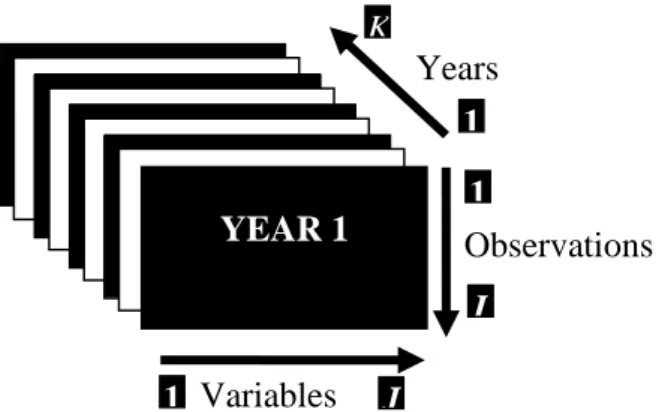
 Three-way data tables: There are data tables that can be presented in a (three way, three mode or third dimension) data structure as shown in Figure 2.1. A particular remark is that all the tables must have the two dimensions in common (rows and columns) (Tormod, et al., 2010).

(12)

5 Figure 2.1. General structure of three-way data sets

In Figure 2.1 for each year (k), there is a data table consisting of measurements for a number of J attributes and a number of I observations. In most of the cases, multiway data tables contain the same number of rows and same number of columns.

 Multi-Block data tables: They are several data tables that have a common dimension between them, i.e. either the same rows or the same columns, but not necessarily both. Each group of variables, or each matrix, is usually called a block or a configuration and in general is measured on the same observations, as shown in Figure 2.2.

Figure 2.2. General structure of multi-block data tables

In Figure 2.2 for each year (k), there is a data table consisting of measurements for a number of JK attributes, but the number of JK attributes can vary for each

year, and the number of I observations remains the same. Years YEAR 1 _Observations 1 I 1 Variables 1 J K Years YEAR 1 _Observations 1 I 1 K Variables 1 JK

(13)

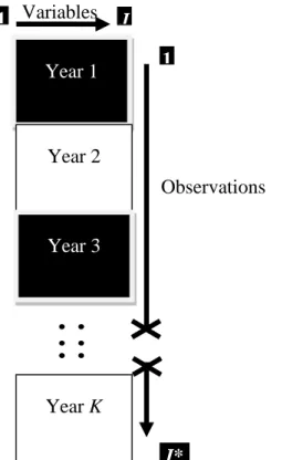
6  Unfolding: It is a way of reordering multiple tables to a pooled matrix as a horizontal or vertical concatenation of matrices (Tormod, et al., 2010). As shown in Figure 2.3 with the same common observations as rows and all tables variables as columns. Figure 2.4 depicts the case of the same common variables as columns and all tables’ observations as rows.

Figure 2.3. The different data tables of the years are put contiguous to each other

Figure 2.4. The different data tables of the years are put on a stack, whose columns are the same variables

Year 1 Year 2 Year 3 Year K

Observations 1 I Variables 1 J* K

X X

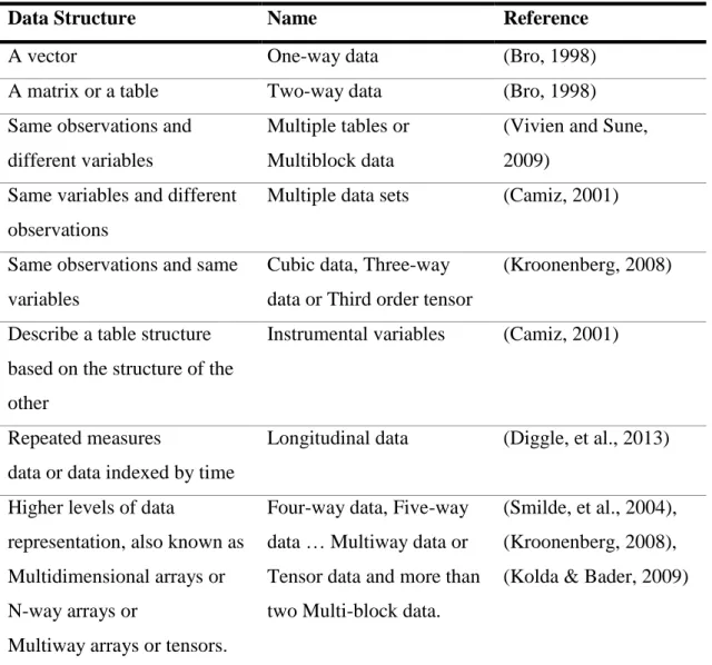
Year 1 Year 2 Year 3 Year K Variables 1 I* Observations 1 J

(14)

7 So, in conclusion according to the particular structure of data, the data sets take different names. For instance the Table 2.1 shows some common structures and names, it is a generalization of the classification of Camiz (2001).

Table 2.1. Names of data sets according to particular structure of data

Data Structure Name Reference

A vector One-way data (Bro, 1998)

A matrix or a table Two-way data (Bro, 1998)

Same observations and different variables

Multiple tables or Multiblock data

(Vivien and Sune, 2009)

Same variables and different observations

Multiple data sets (Camiz, 2001)

Same observations and same variables

Cubic data, Three-way data or Third order tensor

(Kroonenberg, 2008)

Describe a table structure based on the structure of the other

Instrumental variables (Camiz, 2001)

Repeated measures

data or data indexed by time

Longitudinal data (Diggle, et al., 2013)

Higher levels of data

representation, also known as Multidimensional arrays or N-way arrays or

Multiway arrays or tensors.

Four-way data, Five-way data … Multiway data or Tensor data and more than two Multi-block data.

(Smilde, et al., 2004), (Kroonenberg, 2008), (Kolda & Bader, 2009)

Consequently, the methods for analyzing multiblock data are called multitable or multiblock methods. So, these are methods dedicated to analyze simultaneously several tables of data, like Multiblock PCA that applies PCA on a multi-block data.

Therefore, it is important to consider these different structures in order to decide the specific method of data analysis that must be applied such as multiblock methods, 3-way analysis methods, methods on instrumental variables, multiway analysis, and so on.

(15)

8

2.2 Overview of joint Analysis methods of tables

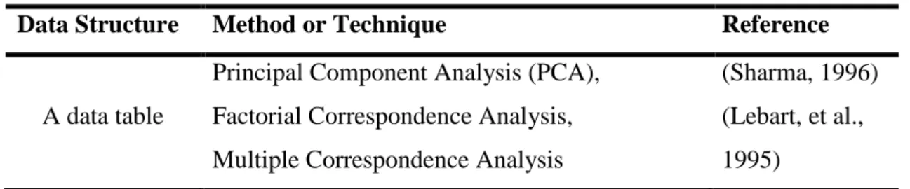
Firstly, the Table 2.2 remembers us the well-known techniques for the analysis of a data table described by numerical or nominal variables.

Table 2.2. Basic techniques for analyzing a data table

Data Structure Method or Technique Reference

A data table

Principal Component Analysis (PCA), Factorial Correspondence Analysis, Multiple Correspondence Analysis

(Sharma, 1996) (Lebart, et al., 1995)

Secondly, there are a lot of possible methods that researchers can consider for the analysis of multiple data tables as shown in Table 2.3, divided in two categories: analysis of multi tables or multiblock and three-way data tables, and methods for two or more multi-blocks data and multi-way data, or a combination of both, like two four-way multiblock data. Most of the methods in Table 2.3 are extensions of Principal Component Analysis.

There is other classification about the overview of analysis methods for multi-group data in Eslami, et al. (2013).

Table 2.3. Original methods and obtained of original methods

Multiblock or Three-way data

STATIS: Structuring Three-way data sets in Statistics, Dual STATIS

(Lavit, et al., 1994)

CCSWA: Common Components and Specific Weights Analysis, Dual CCSWA

(Qannari, et al., 2001)

MUDICA: Multiblock Discriminant Correspondence Analysis

(Abdi, et al., 2010) DACP: Double Principal Component Analysis (Bouroche,

(16)

9 Table 2.3. Original methods and obtained of original methods (cont.)

Multiblock or Three-way data

Multi-Block PCA or Multi-Groups PCA (Derks, et al.,

2003) MFA: Multiple Factor Analysis, also called

Multiple Factorial Analysis, Dual-MFA

(Escofier and Pagés, 1994)

GPA: Generalized Procruste Analysis, Dual GPA (Gower, 1975) Several Multi-blocks or Multi-way data

GOMCIA: Generalized Orthogonal Multiple Co-Inertia Analysis, it is a Partial Least Squares regression or PLS-based method

DO-ACT: DOuble-Analyse Conjointe de Tableaux, or Double-STATIS is a

generalization of STATIS

HMFA: Hierarchical Multiple Factor Analysis (Le Dien and Pagés, 2003) MMCovC: Multiway Multiblock Covariate

Component

(Smilde, 2000)

PARAFAC: Parallel Factor Analysis, PARAFAC-family and derivatives models

(Acar and Yener, 2009) Tucker,

Tucker-family and derivatives models.

(Acar and Yener, 2009)

Tensor Data Analysis (Kolda and

Bader, 2009) STATIS-4 an extension of STATIS and

DO-ACT

(Sabatier and Vivien, 2008)

(17)

10

2.3 Related works about STATIS

Based only on STATIS methodology as a common framework, some methods of joint analysis of tables have been developed, like DO-ACT, STATIS-4 and others (Abdi, et al., 2012).

Also there are some applications of this method in several areas, for example: Gonçalves (2010) studied the performance or evolution of economic activities in Portugal analyzing the information obtained along the years by Bank of Portugal and identifying differences and similarities between years and trends over time for those activities; Brás (2012) uses the information provided by the National Statistical Institute of Portugal (INE) and analyzed the evolution of the construction sector in Portugal in order to offer a better understanding of the Portuguese construction sector over the time; Lourenço (2013) analyzed the vulnerability indicators present in the Early Warning Systems (EWS) of European countries, detecting the main economic weaknesses that contributes to predict the occurrence of a crisis in a certain time horizon; Stanimirova, et al. (2004) applied STATIS for the exploration of three-way environmental data, and compares its performance with Tucker3 and PARAFAC2 methods; González, et al. (2005) analyzed the consumption of electrical power in a hotel during the months that the environmental conditions differ the most, to determine the appropriate actions on the way to its saving; Chaya, et al. (2004) applied this methodology for the analysis of time-intensity profiling data, with sensory attributes of ranch salad dressing as variables, and a set of products as objects; Amendola, et al. (2006) studied the causes of the socio-economic disparities among the European regions; Figueiredo, et al. (2012) analyzed the dynamics and evolution of the structural economic reforms during the period 1989 –1996 where the privatization of state-owned enterprises taking place in the Portuguese banking sector.

Almeida (2012) applied a variant of this methodology called Dual STATIS in a data set that records information about cycles of couples with infertility diagnosis of the Assisted Medical Reproduction Center in Oporto Hospital to understand which variables contribute the most to the differences between the groups of couples. The method allowed us to discover a greater proximity between groups composed of couples who are not pregnant and a greater distance between the groups of couples who become pregnant.

Also, Coquet et al. (1996) adapted STATIS, obtaining significant acceleration to study and characterize the internal molecular motions and conformations from a large

(18)

11 number of molecular dynamics sets of coordinates, when simulated in a solution by molecular dynamics techniques.

2.4 OECD and the Better Life Index

There is a lot of interest for determining the well-being of societies, and one of the primary indicators is the Gross Domestic Product (GDP) that is used for measuring the condition of a country´s economy. We use GDP sometimes for judging the success of countries but the problem is that GDP does not include neither a social dimension nor the environmental problems, like air pollution and water quality. GDP is a tool to support us in measuring the economic performance, but it is not a measure of our well-being, so it is necessary to define a different way to measure the success of countries or of our societies, that complements GDP.

Today we have other approaches to measure the success of countries, like the Better Life Index created by OECD and the Social Progress Index created by Social Progress Imperative organization.

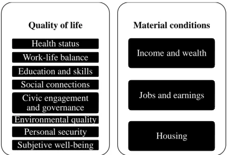
The Organization for Economic Co-operation and Development (OECD) has been interested in measuring well-being and the progress of countries taking into account outcomes about people’s lives rather than economic aspects, so the OECD since May 2011 has launched the OECD Better Life Initiative. It focuses on eleven aspects or dimensions of life that matter to people to form the OECD well-being framework with a set of well-being indicators as Figure 2.5 depicts (OECD, 2013).

(19)

12 Figure 2.5. The OECD well-being conceptual dimensions. Source: (OECD, 2013)

By using these dimensions with some well-being indicators, the OECD Better Life Initiative has designed an interactive web application called the Better Life Index (BLI) for measuring the many things that improve individual well-being allowing users to set their own weights on the domains and create Your Better Life Index by the interactive tool. Additionally it allows people to measure and compare well-being across countries based on those eleven topics essential to the quality of life.

Figure 2.6 shows the interactive tool with flowers representing members of the OECD as well as important partners; each flower has eleven petals one for each dimension in the index. By using interactive tool box, we can begin to create Your Better Life Index according to what is important to us and it is possible to increase or decrease the priority given to each topic by adjusting sliders from the left to right. Countries or flowers that move to the top are the ones that perform best according to priorities we set. Petals also change the width reflecting the importance we have given each topic to get a clear view of how countries are different to one another. Additionally, once we have created our Better Life Index we are able to compare with those of other users by country and share with other persons.

Quality of life

Health status Work-life balance Education and skills

Social connections Civic engagement and governance Environmental quality Personal security Subjetive well-being Material conditions

Income and wealth

Jobs and earnings

(20)

13 Figure 2.6. The screenshot of Your Better Life Index web application. The screenshot shows the BLI of countries displayed by rank (OECD, 2015)

Since OECD data of countries are essentially multiblock data tables, multiblock component methods can be used for analyzing differences or similarities between OECD tables. In this thesis the Statis methodology will be applied.

(21)

14

CHAPTER 3 Methodology and Description of the Data Tables

This chapter presents a brief description of the methodology used in this study. The methodology described in this chapter requires that the individuals must be the same for all data tables. Also the individuals (countries), variables and years under study are presented, and the chapter concludes with a preliminary analysis of the data tables.

3.1 STATIS Methodology

The STATIS methodology was firstly developed in the Statistics and Probability Laboratory of the University of Montpellier II by Escoufier (1973) and his team and by L’Hermier des Plantes (1976) and later developed by Lavit (1988) and Lavit, et al. (1994). It lets you extract information from multidimensional data collected in diverse situations or time instants.

The STATIS methodology can be seen as a three-way exploratory analysis methodology or as an extension of Principal Component Analysis for the analysis of multiple data tables that measure sets of variables collected on the same observations. STATIS does not require the data tables to have the same number of columns. When the data tables have the same columns and not the same rows, the Dual STATIS method can be used.

The STATIS method, is a type of multivariate factorial analysis method and its main goal is to search a common structure between the different data tables. It follows the next steps:

1. STATIS starts with the selection of K data tables collected on the same individuals. Each table (is also called a block, a study, a subtable, a configuration or data set) is a data matrix Xk with dimensions: I x Jk, where I is the number of

individuals, observations or a sample (e.g. number of countries in this case) and Jk the number of quantitative variables, measurements or attributes collected on

the individuals for the kth table (at time k). Each data matrix can be preprocessed (e.g., centered by column, normalized) separately or on unfolded data, and STATIS may be run with standardized or non-standardized variables.

(22)

15 2. The principal step of the STATIS is called Interstructure analysis and compare the spatial distribution of the individuals of the K matrices to each other, using the strategy described next.

2.1. To each matrix Xk, we associate its I x I cross-product matrix defined as

Wk = Xk XkT, with k = 1,...,K, (3.1)

where ‘T’ means transpose of a matrix. So, Wk is the cross-product matrix between

individuals for the kth data table and it is considered as a representative object for this table. Also Wk is considered as a point in the space RIxI.

2.2. To analyze the similarities structure between two matrices Wk and Wk´ we

used the vector correlation coefficient, denoted by RV coefficient, also called Escoufier’s RV coefficient, initially introduced by Escoufier (1973), and represents the cosine between matrices, it means the similarity or correlation between squared symmetric matrices, and can be interpreted as a generalization of the squared Pearson correlation coefficient; for the kth and the k´th data tables, the RV coefficient is defined as

𝑅𝑉_k,k´ = trace (𝐖𝐤𝐓𝐖𝐤´)

√trace (𝐖_𝐤𝐓𝐖𝐤)∗trace (𝐖𝐤´𝐓𝐖𝐤´)

𝟐 , (3.2)

and, the term trace (W_kTW_k´) defines a scalar product between matrices Wk and

Wk´, called Hilbert-Schmidt inner product or H-S inner product, that enable us to

determine the distance between the matrices.

This is used to calculate the matrix of RV coefficients (K x K) called between matrix cosine or simply RV matrix and denoted by C, to analyze the similarities structure of the matrices. The RV coefficients are non-negative and ranges between 0 and 1, and the closer RV is to 1 means the more similar the two data matrices k and k´ are.

(23)

16 2.3 Perform the eigendecomposition of the positive semi-definite matrix C (often called diagonalization of C) provides an optimal representation of the relative position of the matrices Wk. A matrix is positive semi-definite when it can be

obtained as the product of a matrix by its transpose, this implies the matrix is always symmetric, for instance positive semi-definite matrices include correlation, covariance, and cross-product matrices. Therefore, we can express the matrix C as:

C = UɅUT_, _(3.3)

where U (UTU = I) is the matrix with the normalized eigenvectors of C and Ʌ the diagonal matrix of the eigenvalues of C.

An element of a given eigenvector represents the projection of one table on this eigenvector. Thus the tables can be represented as points in the eigenspace and their similarities can be visualized in the space, like to perform PCA of the non-centered C matrix, which is called Interstructure analysis. The projections are computed as

Y = UɅ1/2_. _(3.4)

2.4 Calculate the Compromise or Consensus matrix (W) which is a weighted average among the K tables to be compared, it is computed as

W = ∑𝐾_𝑘=1𝑎_𝑘W_k , (3.5)

where W (I x I) can be considered as a linear combination of the initial Wk

matrices, and ak is the weight for the kth table, it is obtained from the eigenvector

associated with the highest eigenvalue of the C matrix, and represents what is common to the different tables or the agreement between tables, where tables with larger weight on the first eigenvector are more similar to the other tables.

(24)

17 3. This step is called Intrastructure analysis and perform PCA of compromise matrix that has been defined in the previous step, using the following strategy

3.1. Perform the eigendecomposition of W, again W is a cross-product matrix and therefore its eigendecomposition is equivalent to a PCA and it gives information about the structure or similarities of the set of individuals. Their distribution can be visualized by the principal components and the representation is called compromise score plot, so the eigendecomposition of the compromise gives

W = VʘVT_, _(3.6)

where V (VTV = I) is the matrix with the normalized eigenvectors of C and ʘ is the diagonal matrix of eigenvalues, thus the factor scores of the compromise matrix for the individuals are

Y = Vʘ1/2_. _(3.7)

In the Y matrix, each row represents an observation and each column is a component.

3.2. Additionally, it is possible to project each Wk matrix on the compromise plot

and develop the trajectories of the individuals. Also is possible integrate the original variables and the factors of the compromise, and plot the variables on the circles of correlations.

(25)

18 Figure 3.1. The main steps of STATIS method

Xk X1 Observations 1 I 1 K Variables 1 JN Preprocessed Matrix unfolding, centered, normalized

Compute Cross-product matrix

Wk = Xk XkT

Compute the H-S inner product

<Wk,Wk´>H-S= trace(W_kTW_k´)

Compute the Vector Correlation coefficient

𝑅𝑉k,k´= trace (WkTWk´) √trace (W_kT_W k) ∗ trace (Wk´TWk´) 2 Create RV matrix C C: positive semi-definite matrix

PCA of C

Plot the projections (Y) of the tables

Obtain set of weights (ak) from the first eigenvector of C

Compute the Compromise matrix W

W = ∑𝐾𝑘=1akWk

PCA of Compromise matrix

Plot the compromise factor scores on the Compromise Plot Project each data table on the compromise plot

for representing trajectories of individuals Plot original variables and compromise on

(26)

19

3.2 Variables and Countries

This thesis uses Better Life Index datasets from the statistical databases online platform of the OECD (OECD, 2015), which includes data for the world’s most developed countries and also for some emerging countries that are members of the Organisation for Economic Cooperation and Development, or OECD.

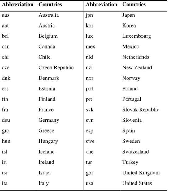
The Better Life Index dataset deals with data pertinent to measure well-being and social progress of the countries. The 34 Member countries are depicted in Table 3.1.

Table 3.1. The OECD Members countries and their ISO codes

Abbreviation Countries Abbreviation Countries

aus Australia jpn Japan

aut Austria kor Korea

bel Belgium lux Luxembourg

can Canada mex Mexico

chl Chile nld Netherlands

cze Czech Republic nzl New Zealand

dnk Denmark nor Norway

est Estonia pol Poland

fin Finland prt Portugal

fra France svk Slovak Republic

deu Germany svn Slovenia

grc Greece esp Spain

hun Hungary swe Sweden

isl Iceland che Switzerland

irl Ireland tur Turkey

isr Israel gbr United Kingdom

ita Italy usa United States

(27)

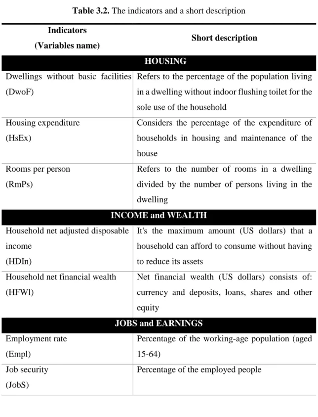
20 Based on experience, OECD defines 11 dimensions or topics (see Figure 2.5) and these topics of the Index are currently based on one to four indicators, so they are 24 indicators in all for measuring the well-being and social progress of the 34 countries. Within each topic, the indicators are averaged with equal weights. The indicators (variables) are shown in Table 3.2.

Table 3.2. The indicators and a short description Indicators

(Variables name) Short description

HOUSING

Dwellings without basic facilities (DwoF)

Refers to the percentage of the population living in a dwelling without indoor flushing toilet for the sole use of the household

Housing expenditure (HsEx)

Considers the percentage of the expenditure of households in housing and maintenance of the house

Rooms per person (RmPs)

Refers to the number of rooms in a dwelling divided by the number of persons living in the dwelling

INCOME and WEALTH

Household net adjusted disposable income

(HDIn)

It's the maximum amount (US dollars) that a household can afford to consume without having to reduce its assets

Household net financial wealth (HFWl)

Net financial wealth (US dollars) consists of: currency and deposits, loans, shares and other equity

JOBS and EARNINGS

Employment rate (Empl)

Percentage of the working-age population (aged 15-64)

Job security (JobS)

(28)

21 Table 3.2. The indicators and a short description (cont.)

Indicators

Long-term unemployment rate (LUnp)

Refers to the number of persons who have been unemployed for one year or more as a percentage of the labour force (the sum of employed and unemployed persons).

Personal earnings (PEar)

Refers to the average annual wages. (US dollars)

SOCIAL CONNECTIONS or COMMUNITY

Quality of support network (QSNw)

It's a measure of perceived social network support. (Percentage)

EDUCATION and SKILLS

Educational attainment (EdAt)

Percentage of the adult population (aged 25 to 64) holding at least an upper secondary degree Student skills

(SdSk)

Students’ average score in reading, mathematics and science as assessed by the OECD’s Programme for International Student Assessment (PISA)

Years in education (YsEd)

Average duration (years) of education in which a 5 year old child can expect to enroll during his/her lifetime until the age of 39

ENVIRONMENTAL QUALITY

Air pollution (AirP)

Micrograms per cubic meters of annual concentrations of particulate

Water quality (WatQ)

Percentage of people's subjective appreciation of the quality of the water.

CIVIC ENGAGEMENT and GOVERNANCE

Consultation on rule-making (CoRl)

It’s a weighted average of yes/no answers to various questions on the existence of law consultation by citizens

(29)

22 Table 3.2. The indicators and a short description (cont.)

Indicators

Voter turnout (VoTr)

Percentage of people that cast a ballot

HEALTH STATUS

Life expectancy (LfEx)

Years old on average people could expect to live Self-reported health

(SHth)

Percentage of the population aged 15 years old and over who report “good” or better health.

SUBJETIVE WELL-BEING or LIFE SATISFACTION

Life satisfaction (LfSa)

Average score of people's evaluation of their life as a whole

PERSONAL SECURITY or SAFETY

Assault rate (Aslt)

Percentage of people declaring having been assaulted or mugged

Homicide rate (Homd)

Rate of deaths due to assault

WORK-LIFE BALANCE

Employees working very long hours

(EWkL)

Percentage of dependent employed whose usual hours of work per week are 50 hours or more

Time devoted to leisure and personal care

(ToLe)

Number of hours per day spent on leisure and personal care

So far, the individuals (34 countries) and variables (24 indicators) have been described, then the 5 data tables used for measuring the well-being of societies came from 2011 to 2015 with the same individuals described by seventeen to twenty-four quantitative variables, are formed as follows:

 The data table from 2011 has 34 individuals or countries presented in rows and 17 variables or indicators presented in columns.

 The data tables from 2012 to 2015 have 34 individuals or countries presented in rows and 24 variables or indicators presented in columns, for each table.

(30)

23

3.3 Preliminary Analysis of the data set

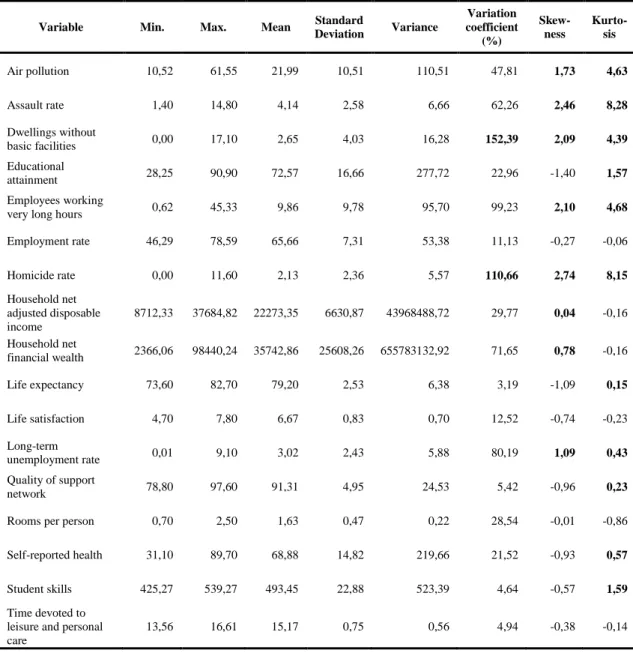
The following tables (Table 3.3 to Table 3.7) represent descriptive statistics for all variables, where each table corresponds to each of the years from 2011 to 2015. In the tables, if the variation coefficient is in bold, that means that the variable has a high dispersion. The variables that are positively skewed have positive skewness coefficient (in bold in the tables) and predominate the low values. The variables with positive kurtosis coefficient (in bold in the tables) indicate that have a distribution more elongated than the normal distribution.

Table 3.3. Descriptive statistics for 2011

Variable Min. Max. Mean Standard

Deviation Variance Variation coefficient (%) Skew-ness Kurto-sis Air pollution 10,52 61,55 21,99 10,51 110,51 47,81 1,73 4,63 Assault rate 1,40 14,80 4,14 2,58 6,66 62,26 2,46 8,28 Dwellings without basic facilities 0,00 17,10 2,65 4,03 16,28 152,39 2,09 4,39 Educational attainment 28,25 90,90 72,57 16,66 277,72 22,96 -1,40 1,57 Employees working

very long hours 0,62 45,33 9,86 9,78 95,70 99,23 2,10 4,68

Employment rate 46,29 78,59 65,66 7,31 53,38 11,13 -0,27 -0,06 Homicide rate 0,00 11,60 2,13 2,36 5,57 110,66 2,74 8,15 Household net adjusted disposable income 8712,33 37684,82 22273,35 6630,87 43968488,72 29,77 0,04 -0,16 Household net financial wealth 2366,06 98440,24 35742,86 25608,26 655783132,92 71,65 0,78 -0,16 Life expectancy 73,60 82,70 79,20 2,53 6,38 3,19 -1,09 0,15 Life satisfaction 4,70 7,80 6,67 0,83 0,70 12,52 -0,74 -0,23 Long-term unemployment rate 0,01 9,10 3,02 2,43 5,88 80,19 1,09 0,43 Quality of support network 78,80 97,60 91,31 4,95 24,53 5,42 -0,96 0,23

Rooms per person 0,70 2,50 1,63 0,47 0,22 28,54 -0,01 -0,86

Self-reported health 31,10 89,70 68,88 14,82 219,66 21,52 -0,93 0,57

Student skills 425,27 539,27 493,45 22,88 523,39 4,64 -0,57 1,59

(31)

24 Table 3.4. Descriptive statistics for 2012

Deviation Variance Variation coefficient (%) Skew-ness Kurto-sis Air pollution 11,00 62,00 22,03 10,56 111,42 47,92 1,78 4,79 Assault rate 1,31 10,98 3,98 2,14 4,59 53,87 1,46 2,87 Consultation on rule-making 2,00 11,50 7,29 2,57 6,63 35,30 -0,23 -0,73 Dwellings without basic facilities 0,00 12,67 2,23 3,34 11,12 149,66 1,93 3,08 Educational attainment 30,00 91,00 73,88 16,41 269,26 22,21 -1,43 1,59 Employees working

very long hours 0,68 43,00 9,76 9,66 93,39 98,97 2,02 3,90

Employment rate 46,00 79,00 65,71 7,38 54,52 11,24 -0,26 0,05

Homicide rate 0,30 19,00 2,12 3,21 10,29 151,03 4,71 24,66

Household net adjusted

disposable income 8618,00 37708,00 22337,15 6720,47 45164783,28 30,09 -0,003 -0,19 Household net financial

wealth 2189,00 102075,00 36074,88 25981,77 675052367,93 72,02 0,87 0,11 Housing expenditure 16,00 29,00 22,09 2,83 8,02 12,82 0,42 0,38 Job security 5,18 25,80 9,76 4,66 21,76 47,78 2,03 4,47 Life expectancy 74,30 83,00 79,76 2,41 5,83 3,03 -1,13 0,24 Life satisfaction 4,90 7,80 6,67 0,80 0,63 11,95 -0,70 -0,61 Long-term unemployment rate 0,01 9,04 2,99 2,39 5,73 80,23 1,09 0,47 Personal earnings 11020,00 52607,00 34033,41 11820,54 139725226,92 34,73 -0,35 -0,87 Quality of support network 69,00 98,00 91,18 5,66 32,03 6,21 -2,12 6,28

Rooms per person 0,90 2,60 1,65 0,45 0,20 27,20 0,05 -0,88

Student skills 420,00 543,00 496,68 26,17 684,95 5,27 -0,86 1,58

Time devoted to leisure

and personal care 13,56 16,06 14,79 0,66 0,43 4,43 0,15 -0,52 Voter turnout 48,00 95,00 73,15 12,41 153,95 16,96 -0,07 -1,06 Water quality 59,00 97,00 85,41 10,47 109,58 12,26 -1,04 0,51

(32)

very long hours 0,66 46,13 10,13 9,99 99,86 98,66 2,07 4,55

Employment rate 48,00 79,00 66,00 7,35 54,06 11,14 -0,17 -0,42

Homicide rate 0,30 23,70 2,23 3,97 15,74 177,70 5,10 27,91

Household net adjusted

disposable income 11039,00 38001,00 22949,47 6693,08 44797288,14 29,16 0,08 -0,47 Household net financial

wealth 6905,00 115918,00 38251,82 27429,71 752389030,39 71,71 1,01 0,70 Housing expenditure 16,00 27,00 21,06 2,57 6,60 12,20 0,34 -0,09 Job security 4,70 25,80 10,49 4,86 23,67 46,38 1,91 3,83 Life expectancy 74,20 82,80 80,07 2,45 6,00 3,06 -1,18 0,34 Life satisfaction 4,70 7,80 6,62 0,86 0,75 13,04 -0,61 -0,65 Long-term unemployment rate 0,01 8,99 3,14 2,62 6,87 83,50 1,14 0,31 Personal earnings 9885,00 54450,00 34466,00 11837,86 140134949,27 34,35 -0,30 -0,86 Quality of support network 73,00 98,00 89,71 5,86 34,40 6,54 -1,43 1,60

Rooms per person 0,90 2,60 1,67 0,43 0,19 25,84 0,00 -0,61

Student skills 420,00 543,00 496,68 26,17 684,95 5,27 -0,86 1,58

Time devoted to leisure

and personal care 11,73 16,06 14,63 0,86 0,73 5,85 -1,30 3,35 Voter turnout 47,00 93,00 71,97 12,18 148,45 16,93 -0,04 -0,73 Water quality 61,00 97,00 84,26 9,32 86,93 11,06 -0,58 -0,17 Years in education 14,90 19,60 17,50 1,20 1,45 6,88 -0,52 -0,09

(33)

very long hours 0,59 43,29 9,86 9,17 84,07 92,97 2,00 4,59

Employment rate 49,00 80,00 66,29 7,58 57,49 11,44 -0,31 -0,37 Homicide rate 0,30 23,40 2,15 3,97 15,76 184,41 4,94 26,57 Household net adjusted disposable income 12850,00 39531,00 23675,94 6744,92 45493980,18 28,49 0,23 -0,56 Household net financial wealth 3317,00 132822,00 39742,29 30091,85 905519452,46 75,72 1,13 1,41 Housing expenditure 16,00 27,00 21,38 2,34 5,46 10,92 0,13 0,44 Job security 2,80 17,70 5,80 2,85 8,10 49,06 2,53 8,95 Life expectancy 74,40 82,80 80,08 2,44 5,94 3,04 -1,16 0,28 Life satisfaction 4,70 7,80 6,64 0,90 0,81 13,56 -0,74 -0,59 Long-term unemployment rate 0,01 14,37 3,41 3,33 11,12 97,71 1,74 2,88 Personal earnings 14653,00 54214,00 35192,65 11890,91 141393857,51 33,79 -0,24 -1,13 Quality of support network 68,00 96,00 89,35 6,41 41,14 7,18 -1,79 3,35

Rooms per person 1,00 2,50 1,69 0,43 0,18 25,33 -0,04 -0,96

Student skills 417,00 538,00 496,94 26,02 676,84 5,24 -1,02 1,77

13,42 16,06 14,88 0,56 0,31 3,75 -0,11 0,83

Voter turnout 49,00 93,00 71,65 11,47 131,45 16,00 0,23 -0,79 Water quality 60,00 97,00 84,56 9,84 96,80 11,64 -0,73 -0,06 Years in education 14,10 19,70 17,49 1,26 1,58 7,20 -0,47 0,32

(34)

very long hours 0,45 40,86 9,38 8,44 71,19 89,92 2,07 5,24

Employment rate 49,00 82,00 66,29 7,80 60,88 11,77 -0,25 -0,21 Homicide rate 0,30 23,40 1,87 3,99 15,96 213,57 5,05 27,41 Household net adjusted disposable income 13085,00 41355,00 24630,18 7101,38 50429550,33 28,83 0,31 -0,36 Household net financial wealth 3251,00 145769,00 42340,26 32204,93 1037157628,75 76,06 1,24 1,94 Housing expenditure 16,00 26,00 21,12 2,36 5,56 11,17 0,17 0,05 Job security 2,40 17,80 5,75 2,83 7,98 49,11 2,74 9,98 Life expectancy 74,60 83,20 80,19 2,43 5,88 3,02 -1,16 0,34 Life satisfaction 4,80 7,50 6,59 0,80 0,64 12,19 -0,75 -0,52 Long-term unemployment rate 0,01 18,39 3,63 3,98 15,85 109,54 2,15 5,18 Personal earnings 16193,00 56340,00 37055,18 12724,46 161911774,94 34,34 -0,15 -1,27 Quality of support network 72,00 96,00 89,62 5,25 27,58 5,86 -1,43 3,10

Rooms per person 1,00 2,50 1,69 0,42 0,18 25,18 0,12 -0,91

Student skills 417,00 542,00 497,15 26,59 706,92 5,35 -0,96 1,73

13,42 16,06 14,88 0,56 0,31 3,75 -0,11 0,83

Voter turnout 49,00 93,00 70,06 12,41 154,00 17,71 0,13 -0,83 Water quality 62,00 97,00 83,79 9,64 93,02 11,51 -0,56 -0,66 Years in education 14,40 19,80 17,57 1,29 1,66 7,33 -0,28 -0,07

So, with the location and dispersion measures presented in the Tables 3.3 to 3.7 is possible identify meaningful changes in the variables during the period under study.

(35)

28 First of all, we can see that the variables have different scales of measurement, giving different dispersion measures, so that we need to standardize the variables when applying the Statis methodology.

We can figure out that there is a significant decrease in the mean of the variable Job security between 2013 and 2014, other variables that decrease in the mean between 2011 and 2015 are Air pollution, Dwellings without basic facilities and Homicide rate; and, the variables that increase in mean are Long-term unemployment rate and Personal earnings.

Secondly, using the variation coefficient (CV) we can compare the dispersion of the variables in a manner that does not depend on the variable's measurement unit, where the higher the CV, the greater the dispersion in the variable. Thus, the Tables 3.3 to 3.7 show that the dispersion of most of the variables was relatively high, indicating the differences between countries regarding to the values in each of these variables. During the period under study the variables with greater CV were Air pollution, Assault rate, Dwellings without basic facilities, Employees working very long hours, Homicide rate, Household net financial wealth, Job security and Long-term unemployment rate. Those that showed less CV were Life expectancy, Student skills and Time devoted to leisure and personal care.

Thirdly, with the Tables 3.3 to 3.7 we can analyze the form of the distribution of each variable, measuring its skewness and measuring whether the data have tails heavier or lighter (like flat) relative to a normal distribution, it is the kurtosis. So, the variables with low negative skewness coefficient or negatively skewed distribution are Educational attainment, Life expectancy and Quality of support network. The variables with high positive skewness coefficient or positively skewed distribution are Air pollution, Assault rate, Dwellings without basic facilities, Employees working very long hours, Homicide rate, Household net financial wealth, Job security and Long-term unemployment rate.

The variables with low kurtosis coefficient have flatter distribution, tend to have lack of outliers, these variables are Rooms per person and Voter turnout. The variables with high kurtosis coefficient have heavier distribution, tend to have outliers, these variables are Air pollution, Assault rate, Dwellings without basic facilities, Employees working very long hours, Homicide rate, Household net financial wealth, Job security, Long-term unemployment rate and Quality of support network.

(36)

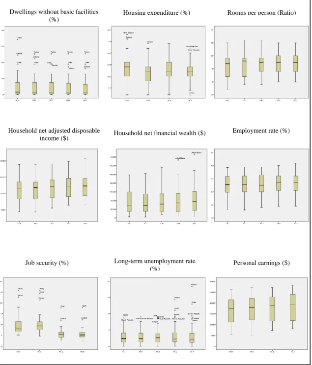
29 In Figure 3.2 we can see the Boxplots of material conditions variables: Dwellings without basic facilities, Housing expenditure, Rooms per person, Household net adjusted disposable income, Household net financial wealth, Employment rate, Job security, Long-term unemployment rate, and Personal earnings.

Figure 3.2. Boxplots of Material Conditions variables

Dwellings without basic facilities (%)

Housing expenditure (%) Rooms per person (Ratio)

Household net adjusted disposable

income ($) Household net financial wealth ($)

Employment rate (%)

Job security (%) Long-term unemployment rate

(37)

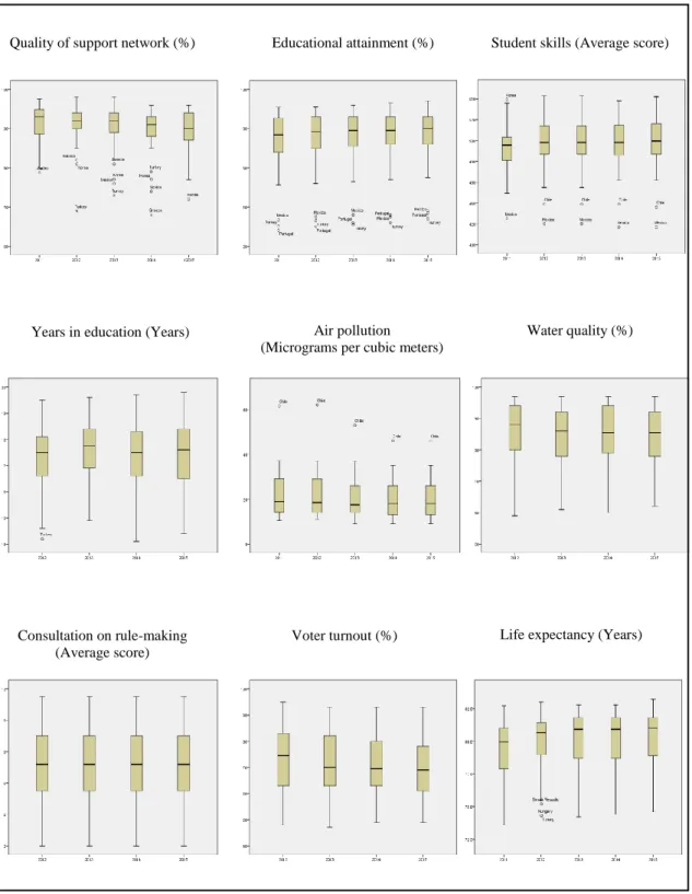
30 In Figure 3.3 we can see the Boxplots of Quality of Life variables: Quality of support network, Educational attainment, Student skills, Years in Education, Air pollution, Water quality, Consultation on rule-making, Voter turnout, Life expectancy, Self-reported health, Life satisfaction, Assault rate, Homicide rate, Employees working very long hours, and Time devoted to leisure and personal care.

Figure 3.3. Boxplots of Quality of Life variables

Quality of support network (%) Educational attainment (%) Student skills (Average score)

Years in education (Years) Air pollution (Micrograms per cubic meters)

Water quality (%)

Consultation on rule-making (Average score)

(38)

31 Figure 3.3. Boxplots of Quality of Life variables (cont.)

Through these boxplots (Figures 3.2 and 3.3) we can diagnose the variability or spread of data and identify moderate outliers (marked with circle) and severe outliers (marked with a star). So, from these boxplots and taking into account the distance between maximum and minimum we can see the dispersion of the variables. Note that the Homicide rate variable is highly concentrated around the median and has 18 outliers during all the period under study.

The country with the highest percentage of dwellings without basic facilities and with employees working very long hours, during all the period is Turkey. For dwellings without basic facilities we have other countries as outliers during all the period, these are Estonia and Chile, and for employees working very long hours the outliers are Japan in 2011-2013, Korea in 2011-2014 and Mexico: 2011-2015.

Self-reported health (%) Life satisfaction (Average score) Assault rate (%)

Homicide rate (Ratio) Employees working very long hours (%)

Time devoted to leisure and personal care (Hours)

(39)

32 Also, Turkey presents the lowest value on time devoted to leisure and personal care from 2013 to 2015, on this variable Mexico appears only in 2013.

The variable Job security decreases in the median from 2013 to 2014 and presents the following outliers: Turkey and Korea in 2012-2013, Mexico in 2013, Spain and Greece in 2014-2015.

The variable Long-term unemployment rate has to Spain and Slovak Republic as outliers countries in all the period, Greece and Ireland are outliers from 2013 to 2015 and Portugal in 2015. Note that Greece is an extreme outlier from 2014 to 2015 and Spain in 2015.

The country with the highest value on assault and homicide rate is Mexico. Also Chile was a moderate outlier in 2011 and 2012 on assault rate, and is an outlier during all the period on homicide rate except in 2012. The highest value of air pollution has Chile during all the period. The United States and Estonia are outliers on homicide rate during all the period.

The countries with the lowest average score on student skills are Mexico and Chile during all the period, while Korea was the highest in 2011.

The country with the lowest value from 2012 to 2015 on Self-reported health variable is Japan. Portugal and Korea appears in 2015, like moderate outliers.

The variable Quality of support network has the following countries as outliers: Turkey in 2011-2014, Mexico in 2014, Korea in 2012-2015 and Greece in 2013-2014.

The variable Educational attainment in all the period has the following moderate outliers: Mexico, Portugal and Turkey.

(40)

33

CHAPTER 4 Results of the STATIS Methodology

This Chapter introduces the results obtained by the application of the Statis methodology to the OECD countries in the period under study, considering the indicators (variables) of well-being.

The results are presented following the main steps of STATIS methodology allowing the analysis of a possible common structure for the data tables that best represents the similarities among the years and, the evolution of the OECD countries described by the variables considered in the study. The data were centered and reduced because the variables are heterogeneous, with different units.

4.1. Interstructure

In the first phase of the Statis method we compute the cross-product matrix between countries (individuals) for each data table with their indicators (variables) of well-being as a representative object of each table, corresponding to each year under study. Then, a global comparison between data tables is done using the coefficient of vector correlation (RV coefficient), in which we conclude what years are more similar and what are more different.

So, through the analysis of the Tables 4.1 and 4.2 about the RV coefficients and the Euclidean distances, respectively, we can conclude that the years 2012 and 2013, 2014 and 2015 are the closest, with a RV coefficient of 0,98, and a distance between these years of 0,19 and 0,18 respectively; while the pairs of years 2011 and 2014, 2011 and 2015 are the most different, with a RV coefficient of 0,92, and a distance between these years of 0,41.

(41)

34 Table 4.1. Matrix of the RV coefficients

Years 2011 2012 2013 2014 2015 2011 1,00 2012 0,95 1,00 2013 0,94 0,98 1,00 2014 0,92 0,95 0,97 1,00 2015 0,92 0,95 0,96 0,98 1,00

Table 4.2. Matrix of the Euclidean distances

Years 2011 2012 2013 2014 2015 2011 0,00 2012 0,32 0,00 2013 0,35 0,19 0,00 2014 0,41 0,30 0,25 0,00 2015 0,41 0,33 0,29 0,18 0,00

By diagonalization of the matrix of RV coefficients, we obtain a system of axes associated to five eigenvalues as well as the percentage of inertia explained by each axis and the percentage of cumulated inertia (Table 4.3). Thus, from Cattel’s and Pearson’s criterion we selected the first two components, because the first two components explain 83,55% of the inertia.

Table 4.3. Eigenvalues, Inertia and Cumulative Inertia of the Interstructure

Axes Eigen- values Inertia Explained (%) Cumul. Inertia (%) 1 0,11 55,62 55,62 2 0,06 27,93 83,55 3 0,02 8,74 92,29 4 0,01 6,74 99,03 5 0,00 0,97 100,00

(42)

35 So, we can see in the Figure 4.1, in the plan defined by the first and second axes, the short distance between the years 2012 and 2013, 2014 and 2015 which indicates proximity or similarity between these years, while the years 2011 and 2014, 2011 and 2015 are more distant between them, and which show the same results we had from Table 4.1 and 4.2.

Figure 4.1. Centred Interstructure Euclidean Image

4.2. Intrastructure

In this step, we compute the compromise matrix defined as a linear combination of the objects, weighted by the coordinates of the objects on the first axis of the Interstructure. Table 4.4 contains the scalar products or correlations between normed objects and the Euclidean distances between objects and the compromise, indicating the years closest and the most distant in relation to the compromise.

Thus, through the analysis of the scalar products and the Euclidean distances, we can conclude that the years are highly correlated with the compromise, because in general distances are low and scalar products are high, proving that it is possible to find a common structure; being the year of 2013 the one that has the highest correlation with the compromise, and the year of 2011 the one with the smallest correlation.

(43)

36 Table 4.4. Scalar products and distances to the compromise object

2011 2012 2013 2014 2015

Scalar Products 0,963 0,985 0,989 0,984 0,980

Euclidean Distances 0,272 0,171 0,148 0,180 0,199

Applying PCA to the compromise object, we show in Table 4.5 the eigenvalue associated to each axis, the inertia explained of each axis and the cumulative inertia. From the Cattel’s and Pearson’s criterion, we considered the first seven axes because the first seven axes explain 79,93% of the total inertia.

Table 4.5. Eigenvalues, Inertia and Cumulative Inertia of the first ten axes

Axes Eigen- values Inertia Explained (%) Cumul. Inertia (%) 1,00 0,89 37,55 37,55 2,00 0,30 12,63 50,18 3,00 0,21 9,11 59,28 4,00 0,15 6,37 65,65 5,00 0,13 5,32 70,97 6,00 0,12 5,07 76,04 7,00 0,09 3,89 79,93 8,00 0,09 3,78 83,71 9,00 0,06 2,67 86,38 10,00 0,05 2,14 88,52

Therefore, the following figures: Figures 4.2, 4.3, 4.4, 4.5, 4.6, and 4.7 are the graphical representations for the seven axes, which show the countries’ compromise Euclidean image in the plan defined by the first and second axes [1, 2], the first and third axes [1, 3], the first and fourth axes [1, 4], the first and fifth axes [1, 5], the first and sixth axes [1, 6], and in the plan defined by the first and seventh axes [1, 7], respectively. In Table VI, Annex C, the linear correlation coefficients between the variables and the seven axes are presented.

In these figures, the farthest countries from the center are the countries that most contribute to the formation of the axis and are selected so that the sum of their

(44)

37 contributions to the axis is about 80%. Additionally, all the countries selected for the axis have a contribution greater than the average contribution of a country and are well represented on that axis. The coordinates, absolute and relative contributions of the countries in the first five axes (Annex A) were taken into account for the interpretation of the axes, and for the interpretation of the compromise axes, we determined the linear correlations between the initial variables and the compromise axes, which are in Annex C; that is made next.

Figure 4.2 shows that the countries with the greatest importance on the first axis are Switzerland (che), Canada (can), Turkey (tur), Mexico (mex) and Chile (chl). So, the first axis makes a distinction between Turkey, Mexico and Chile (all with negative coordinates) and the countries Switzerland and Canada (with positive coordinates).

The first axis is positively correlated with the variable Rooms per person (RmPS), Household net adjusted disposable income (HDIn), Employment rate (Empl), Personal earnings (Pear), Quality of support network (QSNw), Water quality (WatQ), Life expectancy (LfEx) and negatively correlated with Dwellings without basic facilities (DwoF), during all period. Therefore, the first axis opposes Switzerland and Canada with high values in variables RmPS, HDIn, Empl, PEar, QSNw, WatQ, LfEx and low value in Dwellings without basic facilities to Turkey, Mexico and Chile with low values in the variables RmPS, HDIn, Empl, PEar, QSNw, WatQ, LfEx and high value in DwoF.

Figure 4.2. Countries’ compromise Euclidean image in the plan [1, 2]

The second axis (see Figure 4.2) opposes Slovak Republic (svk), Hungary (hun), and Greece (grc) (negative coordinates) with Mexico (mex) and Chile (chl) (positive

(45)

38 coordinates). The second axis is negatively correlated with the variable Long-term unemployment rate (LUnp), during all period. Therefore, this axis refers to the number of persons who have been unemployed for one year or more, differentiating countries that have less unemployed persons for one year or more – Mexico, Chile - from countries whose have more unemployed persons for one year or more, as Slovak Republic, Hungary and Greece.

The third axis (see Figure 4.3) opposes Spain (esp) with negative coordinate to the countries Korea (kor) and Japan (jpn) with positive coordinates in this axis. The third axis is negatively correlated with the variable Student skills (SdSk), during all period. Thus, the third axis opposes Spain to Korea and Japan because Spain has high value in variable Student skills, while Korea and Japan have low values in variable Student skills.

The fourth axis opposes Mexico (mex) with negative coordinate to the countries with positive coordinates, like Korea and Japan. The fourth axis is negatively correlated with the variable Homicide rate (Homd), during all period. So, the fourth axis apposes Mexico to Korea and Japan because the Mexico with negative coordinate have high values in Homicide rate (Homd), while the countries Korea and Japan with positive coordinates have low values in Homd.

(46)

39 Figure 4.4. Countries’ compromise Euclidean image in the plan [1, 4]

The variable that is more correlated with the fifth axis is Consultation on rule-making (CoRl) and it is positively correlated, so from Figure 4.5, this axis opposes the countries Chile (chl), Israel (isr) and Japan (jpn) (positive coordinates) with high values in CoRl to the countries New Zealand (nzl), Australia (aus) (negative coordinates) with low values in the variable CoRl.

The variable that is more correlated with the sixth axis is Housing expenditure (HsEx) and it is negatively correlated, so from Figure 4.6 and also by the absolute contributions, this axis opposes the countries Norway (nor) and Denmark (dnk) (positive

(47)

40 coordinates) with low values in HsEx, to USA (usa) (negative coordinate) with high value in the variable HsEx.

Finally, the seventh axis (see Figure 4.7) opposes Greece (grc) and Iceland (isl) with negative coordinates to Estonia (est) with positive coordinate. Seventh axis has a negative correlation with the variable Air pollution (AirP), in all the period. Thus, Greece and Iceland have high values in variable Air pollution, while Estonia has low value in variable Air pollution.